Abstract
This article deals with the study of ultrasound propagation, which propagates the mechanical vibration of the molecules or of the particles of a material. It measures the speed of sound in air. For this reason, the third-order non-linear model of the Westervelt equation was chosen to be studied, as the solutions to such problems have much importance for physical purposes. In this article, we discuss the exact solitary wave solutions of the third-order non-linear model of the Westervelt equation for an acoustic pressure p representing the equation of ultrasound with high intensity, as used in acoustic tomography. Moreover, the non-linear coefficient (being a part of space-dependent coefficient K), has also been investigated in this literature. This problem is solved using the Generalized Kudryashov method along with a comparison of the Modified Kudryashov method. All of the solutions have been discussed with both surface and contour plots, which shows the behavior of the solution. The images are prepared in a well-established way, showing the production of tissues inside the human body.
1. Introduction
Finding the solution to non-linear problems still faces many difficulties in the field of mathematical physics. Non-linear partial differential equations (NPDEs) [1] play a significant role in physical and mathematical models [2]. They define their ranges from gravitation [3] to fluid dynamics [4], describing many different physical systems. They are mostly related to the fact that these types of equations face the problem of finding their integrability. There are almost no pervasive techniques that can be used for all problems, and usually, every separate model works as an individual problem.
Partial differential equations (PDEs) give solutions in an ultimate state from the past few years while, to exemplify the solutions of NPDEs [5], we can write their solutions with some special clarification. To exemplify the most important applications of NPDEs from the historical point of view, we can highlight one of our focuses as the Westervelt equation [6], which is a non-linear mathematical model, widely used for wave propagation, that can be specified by the possible physical measurements leading to over-posed data. Other fundamental models, which can also be mentioned here, are the Euler and Navier–Stokes equations in fluid dynamics [7], non-linear Schrödinger [8], Klein–Gordon equation [9], the Boltzmann equation in gas dynamics [10], and many more.
To write the solutions of NPDEs explicitly [11], we can reduce the given equation to the equation of one dimension, for which, the process of conversion is applied on NPDE to convert it into an ordinary differential equation (ODE).
In the past few years, many analytical and numerical techniques have been projected to obtain solutions for NPDEs, for example, Bernoulli functional methodology [12], the F-expansion technique [13], the auxiliary equation technique [14], the simplest extended equation technique [15], the (G′/G)-expansion technique [16], the sub-ODE technique [1], the generalized Kudryashov technique(GKM) [17], and many more. The collective theme of all these techniques is to convert the PDEs to ODEs using wave transformations [18]. In this field, the study of solitons [19] is playing an important role in constructing various families of analytic traveling wave solutions [20], which defines the dynamics of solitons leaving a remarkable position in non-linear optics. According to some theoretical research, various modes of plasma (i.e., periodic, rational, solitons, shock-like, explosive) [21] show wave propagation in different natures of non-linear waves.
The reason behind choosing the generalized form of the Kudryashov method is that it approaches the most consistent solutions of the NPDEs. It is also a very useful and efficient approach to finding the solutions to non-linear evolution equations. The modified Kudryashov method is a very strong solution scheme that shows many ways towards the exact solution to the NPDE problem in mathematical physics and biology. Due to the efficient work of this method in the field of mathematics, it has received significant attention towards it. Similarly, a higher-order non-linear Schrödinger equation (NDNLSE) can be solved with the help of this powerful method. It is a successful application that can be performed in several works just like in [22,23].
Ultrasound imaging [24,25] is being used in a well-established way to produce pictures of tissues inside the body of human beings. They are modeled in non-linear wave equations with high intensity.
In many medical and industrial applications, high intensity-focused ultrasound (HIFU) is one of the crucial procedures, which uses high-energy sound waves directly at an area of abnormal tissues of the body to tighten and lift the skin. It also treats tremors, uterine fibroids, and tumors in certain conditions. It includes ultrasound or welding, thermotherapy, sonochemistry, and lithotripsy.
For the purpose of medical imaging, a spatially varying coefficient can be used, which is called acoustic nonlinearity parameter tomography [26]. High-intensity ultrasound propagation [27] is being described with this parameter, which appears in the form of PDEs. These related imaging problems thus become a coefficient identification for them.
Considering the imaging task in the form of the Westervelt equation, consists of an identified K in the acoustic pressure p formulation, represented as:
It can also be formulated in terms of the acoustic velocity potential as:
with .
Here, p is the acoustic pressure, b is the diffusivity of sound, and c is the known constant, which represents the speed of sound. In the above equations, the K and have the following interdependence where signifies the parameter of nonlinearity, is working as the mass density, and acting as bulk modulus, where .
The spatial domain is supposed to be smooth and bounded on which the given PDEs are assumed to hold.
2. Problem Statement
A Westervelt equation in pressure formulation with acoustic pressure p, diffusivity of sound b, a known constant c, and , where is the nonlinear parameter, can be written in the following form:
Our goal is basically to solve this PDE analytically. We will find the exact solutions of this equation, without assuming the initial and boundary conditions.
3. Basic Idea
To exemplify the concept of one of the proposed techniques, a nonlinear PDE can be taken as:
which shows that S contains u and its partial derivatives. This PDE can be converted to the following ODE as:
with the help of the following traveling wave transformation:
where is the non-zero arbitrary constant and is the speed of the traveling wave. To demonstrate this method in detail, we can describe it as:
4. The Generalized Kudryashov Method
Suppose the initial solution of Equation (5) is as follows:
with , where ; , where are found to be unknown coefficients; and is the solution of
which can be embodied as
By using the homogeneous balance principle, we obtain the values of P and Q in Equation (7) to attain the polynomial R by substituting the Equations (7) and (8) into Equation (5). Now, equating all the coefficients of polynomials to zero, we obtain the system of algebraic equations. To find the values of unknown coefficients , we solve the system of algebraic equations. Lastly, we develop the solitary wave solution of the suggested equation.
5. The Modified Kudryashov Method
Considering the same non-linear PDE as mentioned above in Section 3 and following the same above mentioned steps, we may have the initial solution of the Equation (5) can be expressed as the finite series as follows:
with , where ; is found to be an unknown coefficient and is the solution of
which can be embodied as
Note that a is any random constant number.
With the help of the homogeneous balance principle, we obtain the value of P in Equation (10) to attain the polynomial R by substituting Equations (10) and (11) into Equation (5). Now we will equate all the coefficients of polynomials to zero to obtain the system of algebraic equations. Now, to find the values of unknown coefficients , we solve the system of algebraic equations. Lastly, we develop the solitary wave solution of the suggested equation.
6. Applications of the Generalized Kudryashov Method on the Westervelt Equation
Using the wave transformation , we can reduce Equation (3) to the ODE as follows:
To find the solution of the tackled model, we balance and by using the homogeneous balance principle to find the value of and found it to be . Since M is a free parameter, we can set it as , which allows us to set the value of N as . Thus, the solution of Equation (13) takes the form:
7. Comparison with the Modified Kudryashov Method on the Westervelt Equation
Applying the modified form of the Kudryashov method on the Westervelt equation to have a comparison between both method results. We may have the following cases after applying the modified Kudryashov method:
Case I: When
where is the wave speed. Substituting these values in Equation (14) using Equation (9), we obtain the final solution as:
where and is an arbitrary constant.
Case II: When
Substituting these values in Equation (14) using Equation (9), we obtain the final solution as:
where and is an arbitrary constant.
Case III: When
Substituting these values in Equation (14) using Equation (9) we obtain the final solution as:
where and is an arbitrary constant.
The graphical behavior of solitons of the above-mentioned Westervelt equation has been shown in the figures given below. To understand the physical properties of the attained outcomes, some of the resultants are represented by selecting different values of parameters. For example, Figure 1, Figure 2, Figure 3 and Figure 4 are representing the behavior of solitons in the form of surface and contour plots where the parameters are mentioned below the figures.

Figure 1.
The above graphs show the graphical illustration of solitons in the form of the surface plots (on the left) and contour plots (on the right side) of acoustic pressure p where the values of parameters are mentioned below in A. This graph represents the behavior of solitons of Equation (17) which is a lump wave with a background or a lump wave with a kink background.
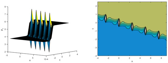
Figure 2.
The above graphs show the graphical illustration of solitons in the form of the surface plots (on the left) and contour plots (on the right side) of acoustic pressure p where the values of parameters are mentioned below in B. This graph represents the behavior of solitons of Case I Equation (19) which is a mixed lump train wave with a kink background, the dynamical feather wave (as velocity and amplitude) has retained the same value along the x-axis.

Figure 3.
The above graphs show the graphical illustration of solitons in the form of the surface plots (on the left) and contour plots (on the right side) of acoustic pressure p where the values of parameters are mentioned below in C. This graph represents the behavior of solitons of Case II Equation (21) showing 3D and their contour plots of breathers distribution under solitary wave background.

Figure 4.
The above graphs show the graphical illustration of solitons in the form of the surface plots (on the left) and contour plots (on the right side) of acoustic pressure p where the values of parameters are mentioned below in D. This graph represents the behavior of solitons of Case III Equation (23) which shows 3D and their contour plots of breathers distribution under solitary wave background.
A. (−4:0.1:9, −4:0.5:2.5).
B. (−4:0.1:9, −4:0.5:2.5).
C. (−4:0.1:9, −4:0.5:2.5).
D. (−4:0.1:9, −4:0.5:2.5).
8. Conclusions
In this paper, the generalized Kudryashov and modified Kudryashov methods were applied to a Westervelt equation showing ultrasound imaging, which produces different pictures of human body tissues. It includes the details of the Westervelt equation, which propagates the imaging of highly intense ultrasound waves. We have found the exact solutions and discussed different cases that represent traveling waves both mathematically and graphically. All possible solutions have been accessed with different types of solitons to obtain the traveling wave solution with different parametric values. The above work clearly shows the efficient applications of NPDEs.
Note: In the sequel of finding better solutions, if we take this problem in the time fractional partial differential equation, then the fractional parameter can be adjusted according to the problems on the physical side. Therefore, we recommend for the future and for ourselves to consider the fractional version of this problem and find whether the solutions are comparable and how they are better convergent w.r.t the comparison of the integer order or the fractional order PDEs.
Author Contributions
S.G., Conceptualization; N.A., Data curation; M.S.I., Formal analysis; A.A., Investigation; M.B., Methodology and M.D.l.S., Supervision. All authors have read and agreed to the published version of the manuscript.
Funding
The authors are grateful to the Basque Government for its support through Grants IT1555-22 and KK-2022/00090; and to MCIN/AEI 269.10.13039/501100011033 for Grant PID2021-1235430B-C21/C22.
Conflicts of Interest
The authors declare no conflict of interest.
References
- Alharbi, A.; Almatrafi, M. Riccati–Bernoulli sub-ODE approach on the partial differential equations and applications. Int. J. Math. Comput. Sci. 2020, 15, 367–388. [Google Scholar]
- Logan, J.D. An Introduction to Nonlinear Partial Differential Equations; John Wiley & Sons: Hoboken, NJ, USA, 2008; Volume 89. [Google Scholar]
- De Sabbata, V.; Gasperini, M. Introduction to Gravitation; World Scientific Publishing Company: Singapore, 1986. [Google Scholar]
- Batchelor, C.K.; Batchelor, G. An Introduction to Fluid Dynamics; Cambridge University Press: Cambridge, UK, 2000. [Google Scholar]
- Rosinger, E.E. Generalized Solutions of Nonlinear Partial Differential Equations; Elsevier: Amsterdam, The Netherlands, 1987. [Google Scholar]
- Karamalis, A.; Wein, W.; Navab, N. Fast ultrasound image simulation using the westervelt equation. In Proceedings of the International Conference on Medical Image Computing and Computer-Assisted Intervention, Beijing, China, 20–24 September 2010; Springer: Berlin/Heidelberg, Germany, 2010; pp. 243–250. [Google Scholar]
- Hughes, T.J.; Franca, L.P.; Mallet, M. A new finite element formulation for computational fluid dynamics: I. Symmetric forms of the compressible Euler and Navier-Stokes equations and the second law of thermodynamics. Comput. Methods Appl. Mech. Eng. 1986, 54, 223–234. [Google Scholar] [CrossRef]
- Delfour, M.; Fortin, M.; Payr, G. Finite-difference solutions of a non-linear Schrödinger equation. J. Comput. Phys. 1981, 44, 277–288. [Google Scholar] [CrossRef]
- Detweiler, S. Klein-Gordon equation and rotating black holes. Phys. Rev. D 1980, 22, 2323. [Google Scholar] [CrossRef]
- Reitz, R.D. One-dimensional compressible gas dynamics calculations using the Boltzmann equation. J. Comput. Phys. 1981, 42, 108–123. [Google Scholar] [CrossRef]
- Galaktionov, V.A.; Svirshchevskii, S.R. Exact Solutions and Invariant Subspaces of Nonlinear Partial Differential Equations in Mechanics and Physics; Chapman and Hall/CRC: Boca Raton, FL, USA, 2006. [Google Scholar]
- Kokar, M.M. Coper: A methodology for learning invariant functional descriptions. In Machine Learning; Springer: Berlin/Heidelberg, Germany, 1986; pp. 151–154. [Google Scholar]
- Karaman, B. The use of improved-F expansion method for the time-fractional Benjamin–Ono equation. Rev. Real Acad. Cienc. Exactas Físicas Nat. Ser. A Mat. 2021, 115, 1–7. [Google Scholar] [CrossRef]
- Lv, X.; Lai, S.; Wu, Y. An auxiliary equation technique and exact solutions for a nonlinear Klein–Gordon equation. Chaos Solitons Fractals 2009, 41, 82–90. [Google Scholar] [CrossRef]
- Zayed, E.M.; Shohib, R.M. Optical solitons and other solutions to Biswas–Arshed equation using the extended simplest equation method. Optik 2019, 185, 626–635. [Google Scholar] [CrossRef]
- Bekir, A.; Guner, O.; Bhrawy, A.H.; Biswas, A. Solving Nonlinear Fractional Differential Equations Using Exp-Function and (G’/G)-Expansion Methods. 2015. Available online: https://rjp.nipne.ro/2015_60_3-4/RomJPhys.60.p360.pdf (accessed on 12 October 2022).
- Gaber, A.; Aljohani, A.; Ebaid, A.; Machado, J.T. The generalized Kudryashov method for nonlinear space–time fractional partial differential equations of Burgers type. Nonlinear Dyn. 2019, 95, 361–368. [Google Scholar] [CrossRef]
- Taravati, S.; Eleftheriades, G.V. Four-dimensional wave transformations by space-time metasurfaces. arXiv 2020, arXiv:2011.08423. [Google Scholar]
- Drazin, P.G.; Drazin, P.G.; Johnson, R. Solitons: An Introduction; Cambridge University Press: Cambridge, UK, 1989; Volume 2. [Google Scholar]
- Yokuş, A.; Durur, H.; Nofal, T.A.; Abu-Zinadah, H.; Tuz, M.; Ahmad, H. Study on the applications of two analytical methods for the construction of traveling wave solutions of the modified equal width equation. Open Phys. 2020, 18, 1003–1010. [Google Scholar] [CrossRef]
- Bashir, M.F.; Murtaza, G. Effect of temperature anisotropy on various modes and instabilities for a magnetized non-relativistic bi-Maxwellian plasma. Braz. J. Phys. 2012, 42, 487–504. [Google Scholar] [CrossRef][Green Version]
- Khater, A.; Seadawy, A.; Helal, M. General soliton solutions of an n-dimensional nonlinear Schrödinger equation. Nuovo C. B 2000, 115, 1303–1311. [Google Scholar]
- Kichenassamy, S.; Littman, W. Blow-up surfaces for nonlinear wave equations, I. Commun. Partial. Differ. Equ. 1993, 18, 431–452. [Google Scholar] [CrossRef]
- Wells, P.N. Ultrasound imaging. Phys. Med. Biol. 2006, 51, R83. [Google Scholar] [CrossRef] [PubMed]
- Ross, M.T.; Antico, M.; McMahon, K.L.; Ren, J.; Powell, S.K.; Pandey, A.K.; Allenby, M.C.; Fontanarosa, D.; Woodruff, M.A. Ultrasound Imaging Offers Promising Alternative to Create 3-D Models for Personalised Auricular Implants. Ultrasound Med. Biol. 2022, 48, 450–459. [Google Scholar] [CrossRef] [PubMed]
- Zhang, D.; Gong, X.F. Experimental investigation of the acoustic nonlinearity parameter tomography for excised pathological biological tissues. Ultrasound Med. Biol. 1999, 25, 593–599. [Google Scholar] [CrossRef]
- Zhang, D.; Chen, X.; Gong, X.F. Acoustic nonlinearity parameter tomography for biological tissues via parametric array from a circular piston source: Theoretical analysis and computer simulations. J. Acoust. Soc. Am. 2001, 109, 1219–1225. [Google Scholar] [CrossRef] [PubMed]


Publisher’s Note: MDPI stays neutral with regard to jurisdictional claims in published maps and institutional affiliations. |
© 2022 by the authors. Licensee MDPI, Basel, Switzerland. This article is an open access article distributed under the terms and conditions of the Creative Commons Attribution (CC BY) license (https://creativecommons.org/licenses/by/4.0/).