Multivehicle Point-to-Point Network Problem Formulation for UAM Operation Management Used with Dynamic Scheduling

Abstract

In this paper, we introduce a new formulation of the multivehicle point-to-point network problem to be utilised in urban air mobility (UAM) vertiport-to-vertiport network operations. Vehicle routing problems (VRPs) and their variants have previously been studied and applied in real-world situations, but these problems require additional depot locations, and not all the vehicles can travel to all the locations. In UAM operations, additional depot locations may not be required, and all vehicles can travel to all locations, meaning that existing routing problems are not suitable for application to the management of UAMs. Therefore, we propose a new formulation for UAM vertiport-to-vertiport operation by introducing new constraints. In addition, we integrate dynamic scheduling with the flight mission by controlling cruise speed and waiting in each UAM at each vertiport location to generate an arrival and departure schedule for different vertiports that can avoid collisions and increase the number of vehicles. A computational experiment is conducted using an MILP model, and the results show that although our formulation satisfies the problem definition, the computation time increases exponentially with an increase in the problem size. A case study is conducted in the Seoul area involving five vertiports, with 10- and 15-vehicle scenarios studied. This case study shows that the cruise speed variable is active only for the lower and upper bounds under dynamic scheduling, whereas the waiting time variable can be controlled between user-defined limits that can be applied to the management of vertiport-to-vertiport UAM operations.

1. Introduction

In recent years, enhancements in distributed and electric propulsion have led to new technology in the drone sector and have triggered developments in passenger-carrying aerial vehicles for civil use in urban settings [1,2]. Although urban aerial mobility has accounted for a minor part of the transport landscape for decades through the deployment of helicopters, various novel concepts, mostly involving electrical vertical takeoff and landing (eVTOL) vehicles, now offer advancements that promise to dramatically expand this market and to provide a relevant mode of transport for people over short to medium distances. However, the realisation of commercial and eVTOL-based passenger vehicles, referred to as urban air mobility (UAM), makes it necessary to consider economically viable scenarios for application, in addition to addressing the actual demand for transportation in society as needed. NASA, commercial mobility-on-demand operators, state-funded research institutes [2] and K-UAM (Hyundai’s UAM research centre) are exploring UAM solutions for cities and surrounding regions, and studies such as [2,3,4] have proposed various approaches and operational concepts to allow UAMs to fly safely through the airspace. Ideas that have been proposed to date include a wide range of possibilities, such as allowing UAMs to land at vertiports installed on roofs of existing buildings or within cloverleaf exchanges on freeways. The operation of UAMs has been divided into three categories: city taxi (on-demand flights between any available landing stations) airport shuttle (scheduled flights along defined routes between airports and landing stations) and intercity (scheduled flights along defined routes) [5]. To solve the problem of airspace use, route optimisation between vertiport locations and scheduling plans for each UAM are required.

Commercial airlines operate based on a fixed, predetermined timetable of scheduled and assigned flights. To create this timetable, routes are first developed between cities depending on demand. Depending on these routes, a schedule is generated based on the specific operating restrictions of each airport, such as the fixed schedules available for a given airline. Fleets are then assigned, and a decision is made as to which aircraft will perform each scheduled flight; the best type of aircraft is assigned to each flight to maximise profitability [3]. In contrast, UAM flight operation services have been envisaged as an on-demand aerial travel service but may also be operated based on a fixed, predetermined timetable in the same way as airlines operate scheduled flights [4]. To provide an on-demand aerial travel service, it would be preferrable to consider each UAM flight mission, from takeoff to landing, as a series of flight segments before developing flight schedules. However, these vehicles may be operated in a city with many UAMs, so an optimum route for each UAM and preset schedules are required for flight safety. The increasing complexity of UAMs, as well as the intensification of competition between airlines, has led to a need to create models that include large numbers of routes and restrictions, which can be considered NP-hard integer programming problems [6]. Numerous routing problems have been proposed, such as the travelling salesman problem (TSP) and the vehicle routing problem (VRP), and their variants can be solved to find the optimum route for each vehicle. However, these solutions require additional depot locations, and not all of vehicles can travel to all locations. In the operation of UAMs, additional depot locations are not required, and all vehicles can travel to all locations, meaning that existing routing problems are not suitable for application to UAM operation management.

Therefore, we proposed a new routing problem formulation to be utilized in UAM vertiport-to-vertiport locations by introducing new constraints. However, scheduling is required for safe operation with an increasing number of vehicles and depot locations. Most airline scheduling and assignment problems already specify a time window for departure from and arrival at the airport [7,8], which is known as static scheduling [9]. In UAM operation, landings and departures are assigned to different runways and are sequenced in advance based on their start times, which is known as dynamic arrival and departure scheduling (dynamic AADS) [9]. Unlike other airline scheduling problems [7,8,10], instead of static scheduling, we introduced new constraints for dynamic scheduling, which is controlled by vehicles’ travel speeds and waiting time constants, enabling generation of dynamic arrival and departure scheduling so that UAMs can operate with no collisions with an increasing numbers of vehicles.

2. Motivation

The nature of UAM operations is inherently different from that of ground-based transportation, and new concepts and procedures are currently being developed to ensure the safety and efficiency of such operations, which will take place alongside traditional aviation. New models of operations management are also needed to support strategic and tactical decision making by service providers, such as optimum route planning and fleet scheduling to maximise their preferred objectives. Although these models are critical for UAM operations, researchers are still searching for the best model for use in UAM operations management. Hence, we propose a new point-to-point network formulation by considering existing routing problems and the TSP.

The VRP and TSP have been widely used in recent decades for aerial vehicle applications, robotics, transportation and networking [11]. The difference between them is that the TSP considers a single vehicle that visits multiple customer locations before returning to the depot, with the aim of minimising the total travel time and distance [12], whereas the VRP involves a single depot and can also be interpreted as a multiple TSP (mTSP). The mTSP represents a relaxation of the VRP, in which neither the vehicle capacity nor customer demand are considered, whereas the VRP does consider customer demand [11]. However, the mTSP does not allow for multiple visits and subtours, meaning that the solution to the mTSP can be applied to the VRP [11]. There are several variants of the TSP in real-world applications, such as the single-depot mTSP, the multidepot TSP [11] and the coloured TSP (CTSP) [13]. The VRP also has many variants, such as the single-depot VRP (SDVRP) and the multidepot VRP (MDVRP [11]); in addition, to consider customer satisfaction, time windows can be introduced to the routing problem, yielding the SDVRP with time window (SDVRPTW [14]) and MDVRP with time window (MDVRPTW [15]).

These problems have been addressed by many researchers by adding constraints to real-world applications. The VSP and TSP are seen as NP-hard problems, as the solution space and search space expand exponentially [12]. Hence, many algorithms have been developed to solve these problems, including deterministic, metaheuristic and market-based approaches, with additional approaches, such as fuzzy logic and game theory, that have been studied by many researchers [11]. Shuai et al. solved the classical formulation of the mTSP using the NSGA-II framework [16]. Li et al. proposed a new variant of the MDVRPTW under shared depot resources by introducing new constraints and applied a hybrid genetic algorithm [17]. Calvet et al. developed a metaheuristic algorithm to solve the MDVRP with limited capacity and stochastic demand [18]. Herdianti et al. also solved the VRP with particle swarm optimisation to achieve a satisfactory distribution [12].

However, all of the above formulations adopted an accurate formulation of the mTSP and multidepot routing problem with relaxed capacity and time windows. All vehicles need to start and end at the same depot, and not all vehicles can visit each customer location, as exactly one customer is visited by one vehicle. In addition, the depot locations are different from the customer locations, whereas in the case of UAM operations, the depot and customer are at the same location. For instance, an aircraft travels from A to B, where A is the depot and B is the customer location; however, location B also has an aeroplane that can travel to another location A, in which case B is the depot and A is the customer location. These networks form a point-to-point network model, whereas the classical formulation of the routing problem can be seen as a hub-and-spoke network model after optimisation which can be seen in Figure 1. Hence, a classical formulation of the mTSP or MDVRP is not suitable for UAM operations.

A new formulation is therefore required for application to UAM operations. In addition, scheduling needs to be performed to achieve safe operation. Because most airline scheduling and assignment problems already specify a time window for departure from and arrival at the airport [7,8], this kind of problem is known as static arrival and departure scheduling (static AADS) [9]. Landings and departures are assigned to different runways and are sequenced in advance based on their start times. In dynamic AADS, an incomplete list of landings and departures must be reassigned and sequenced using the first-in–first-out (FIFO) rule when an incoming aircraft enters the depot at an unknown time in the future [9]. AADS has previously been applied to airline and runway scheduling problems [19,20].

Our proposed formulation for a point-to-point network model can be compared with the classical multidepot routing problem by relaxing the capacity constraints, as shown in

Table 1. Characteristics of the travelling salesman and vehicle routing problems, as well as the proposed problem. (✓ mean formulation supported characteristics).

Problem	Departure Station		Vehicles at Each Departure Station		Network Type		Time Window
	Single	Multiple	Single	Multiple	Hub-and-Spoke	Point-to-Point	Fixed	Variable
TSP	✓		✓		✓
mTSP	✓			✓	✓
MD-mTSP		✓	✓	✓	✓
TSPTW	✓		✓		✓		✓
mTSPTW	✓			✓	✓		✓
MDmTSPTW		✓	✓	✓	✓		✓
VRP	✓		✓	✓	✓
MDVRP		✓		✓	✓
VRPTW	✓		✓	✓	✓		✓
MDVRPTW		✓		✓	✓		✓
Proposed method		✓	✓	✓		✓		✓

. Our formulation represents a new type of network in which the time window is variable rather than using a fixed or predetermined time window.

3. Problem Definitions for the Point-to-Point Network and Dynamic Scheduling

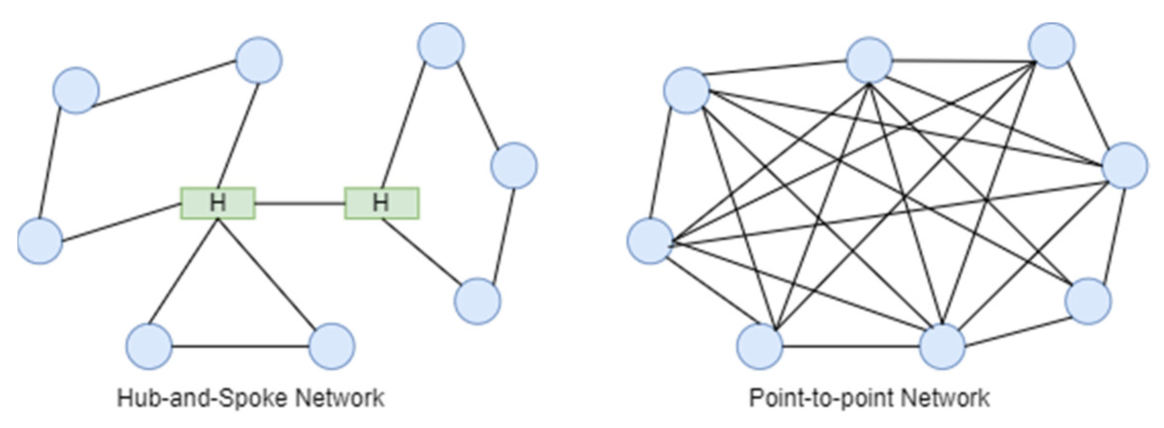
3.1. Problem Definition for Point-to-Point Network

The VRP can be seen as an mTSP in which there are one or more depots with vehicles, such that each customer is visited by exactly one vehicle, forming a hub-and-spoke network. The problem addressed in this paper is a multidepot, multivehicle point-to-point network problem for the vertiport-to-vertiport operation of UAMs. In UAM operations, there may be numerous vertiports and several UAMs at each vertiport, depending on the capacity. Each vehicle at each depot needs to travel to another depot while minimising the cost function. The depot locations of the other vehicles are the customer locations for the vehicles that are at other depot locations, forming a point-to-point network in which each vehicle travels to another depot location exactly once and then returns to its original depot location. An example of our proposed solution is shown in a step-by-step manner in Figure 2.

Figure 2a shows a network of possible routes. Figure 2b shows that vertiport V1 has a vehicle (k1) that travels from V1 to other locations and then returns to its place of origin. Figure 2c shows vertiport V1 with two vehicles, k1 and k2; each vehicle selects a different optimum route and returns to its original location. Figure 2e shows multiple vehicles at multiple depots, which travel to all destinations by selecting different optimum routes and then return to their origin locations. Our proposed solution to the problem is shown in Figure 2f, where each depot has multiple vehicles that travel to all the other depot locations without the need for additional depots for the vehicles.

3.2. Multivehicle Point-to-Point Network with Dynamic Scheduling

Because there are many depots and several vehicles can be at each location, scheduling is required for safe operation. The multivehicle point-to-point network with dynamic AADS proposed in this paper is illustrated in Figure 3. There are two vehicles, UAM1 and UAM2, at the vertiport VD that need to go to other locations via different routes and then to return to the original vertiport, shown in Figure 3a. In addition, a time–space network is presented in Figure 3b that is used for the scheduling and safety of the UAMs. The other vehicles at a vertiport can only leave after the first vehicle leaves and need to wait for a specific time to ensure separation, using the FIFO rule [9]. The arrival times of two vehicles at a vertiport should not be the same, and the departure time from the vertiports should be the same. To control the arrival times at each vertiport, the speed is considered to be variable for the dynamic arrival of different vehicles, as a variable speed is applied for rescheduling by airlines [21] and in the electric VRP [22]. The departure time of two vehicles from a vertiport should not be same. To control the departure time, a variable waiting time is used instead of a fixed, predetermined time stamp as in the existing routing problem. By varying the waiting time at each vertiport, a dynamic departure schedule is achieved. Between each pair of vertiports, the mission flight times and corridors are predicted to satisfy the operation time horizon, as well as the departure and arrival time constraints. This problem is formulated in the following section, and the constraints are explained.

4. Mathematical Formulation

The problem is modelled as a three-index formulation with decision variables, speed variables and time constraints regarding the problem definition, as shown in Figure 3. The mathematical formulation is described below.

Our mathematical model is inspired by a three-index formulation of the MDVRP [23] in which the customer capacity constraints are relaxed. Unlike the formulations of the routing problem and the TSP, the mathematical model incorporates Muiiler–Tucker–Zelim constraints [24] for subtour elimination and considers the travel speed of the vehicles and the constraints on their arrival, departure and waiting times. In addition, route selection constraints are also to each vehicle at each depot in order to select routes that minimise the cost function.

The following assumptions are made for our proposed formulation:

• Each vehicle must leave from and return to the same vertiport;
• All the vehicles need to travel to others vertiport locations;
• Vehicles in the same vertiports must travel by selecting different routes;
• Vehicles in the same vertiports cannot depart at the same time, meaning that the second vehicle needs to travel after the first vehicle after waiting some time;
• Vehicles cannot arrive at the same time to a vertiport, meaning that the second vehicles need to arrive after the first vehicles after waiting some time; and
• All vehicles can travel at varying speeds defined by vehicle specifications.

The following notation is used in this formulation:

• Set and Index:

  $V$	-	Set of vertiports
  $i,j$	-	Index of vertiports
  $K$	-	Set of all vehicles
  $k$	-	Index of vehicles
  $VD$	-	Set of vertiports, $VD=V$
  $K_{VD}$	-	Set of vehicles belonging to each vertiport

• Variables:

  $x_{i,j,k}\in \left\{0,1\right\}$	-	Binary variable that is equal to one if vehicle $k$ travels from $i$ to $j$ and zero otherwise.
  $T{d}_{i,k} \ge 0$	-	Departure time of vehicle $k$ from vertiport $i$, where $i\in V, k\in K$
  $T{a}_{i,k} \ge 0$	-	Arrival time of vehicle $k$ at vertiport $i$, where $i\in V, k\in K$
  $T_{{wait}_{i,k}}\in {ℝ}^{+}$	-	Waiting time of vehicle $k$ at depot $i$, where $i\in V, k\in K$
  $V_k\ge 0$	-	Speed of vehicle $k$, where $k\in K$

• Parameters;

  $d_{i,j}\in {ℝ}^{+}$	-	Distance between $i$ and $j$, where $i\in V, j\in V$
  $V_{max}$, $V_{min}\in {ℝ}^{+}$	-	Maximum and minimum speeds of vehicles
  $T_{{wait}_{max}}$$T_{{wait}_{min}}$	-	Maximum and minimum waiting times
  $n{K}_{VD}$	-	Number of vehicles at each vertiport
  $n{V}_{VD}$	-	Number of vertiports

The objective function is written as follows:

Objective:

$$\min {\displaystyle \sum }_j^V{\displaystyle \sum }_i^V{\displaystyle \sum }_k^K{c}_{i,j}{x}_{i,j,k} \forall k\in K, i\in V, j\in V$$

(1)

The objective is to minimise the total routing cost of all vehicles. The cost function can be selected depending on the user-defined cost function from one vertiport to another. The following constraints are required to complete the model.

$${\displaystyle \sum }_i^V{x}_{i,j,k}=1, \forall k\in K, j\in V$$

(2)

Constraint (2) allows each vehicle to enter all vertiports only once.

$${\displaystyle \sum }_i^V{x}_{i,j,k}=1, \forall k\in K, i\in V.$$

(3)

Constraint (3) allows all vehicles to leave from all vertiports only once.

$${\displaystyle \sum }_i^V{x}_{i,h,k}-{\displaystyle \sum }_j^V{x}_{h,j,k}=0, \forall k\in K, h\in V.$$

(4)

Constraint (4) is a route continuity constraint, which means that if a vehicle enters a location, it must also leave that location.

$$x_{i,j,k+1} \ge x_{ijk}+1-\mathit{M} \left(1-x_{i,j,k+1}\right), \forall i\in V, j\in V, k\in K_{VD}$$

(5)

Constraint (5) ensures that different routes are selected for each vehicle at the same vertiport, as illustrated in Figure 3a. UAM1 and UAM2 are at one vertiport (VD); if UAM1 selects a route from VD to depot 1, UAM2 must select another route from the vertiport. This condition is satisfied by multiplying by a large constant number (M), and the route selected by UAM2 will be $x_{i,j,k+1}=1$, whereas UAM1 is $x_{i,j,k+1}=0$ from the origin to the other locations. The constant (M) is also used for subtour elimination in the VRP and TSP [23,24].

$${\displaystyle \sum }_j^V{x}_{i,j,k} \le 1 \forall i\in VD, k\in K_{VD}$$

(6)

Constraint (6) ensures that each vehicle leaves from the depot no more than once.

$${\displaystyle \sum }_i^V{x}_{i,j,k} \le 1 \forall j\in VD, k\in K_{VD}$$

(7)

Constraint (7) ensures that each vehicle arrives at a depot no more than once.

$${\displaystyle \sum }_j^V{x}_{i,j,k}=0 \forall j\in VD, k\notin K_j$$

(8)

Constraint (8) ensures that a vehicle cannot leave from a depot other than its origin.

$${\displaystyle \sum }_i^V{x}_{i,j,k}=0 \forall j\in VD, k\notin K_j$$

(9)

Constraint (9) ensures that a vehicle cannot return to a depot other than its origin.

Equations (1)–(9) constitute a point-to-point network problem similar to that shown in Figure 2f. Unlike other problems, such as the TSP and VRP, each location is reached by only one vehicle, and the vehicle cannot travel from one depot to another. In this scenario, all vehicles need to travel to other locations, even those that are depots for other vehicles, which creates a complicated routing problem. For the operation of UAMs with this kind of complex routing, optimum scheduling is required. The following time constraints are therefore introduced to solve the dynamic AADS problem shown in Figure 3b.

$$T{a}_{j,k}\ge \left(t{d}_{i,k}+T{r}_{i,j,k}\right)-\mathit{M}\left(1-x_{i,j,k}\right), \forall i\in V, j\in V, k\in K$$

(10)

$$T{r}_{i,j,k}=\mathit{TravelTime}\left(i,j,V_{i,j,k}\right) \forall i\in V, j\in V, k\in K$$

(11)

$$\mathit{TravelTime}\left(i,j,V_{i,j,k}\right)=\raisebox{1ex}{$d_{i,j}$}\!\left/ \!\raisebox{-1ex}{$V_{i,j,k}$}\right. \forall i\in V, j\in V, k\in K$$

(12)

Constraints (10) and (11) allow UAMs to arrive at different times $\left(T{a}_{j,k}\right)$ when travelling from location $i$ to location $j$ by controlling the speed of each vehicle. The arrival time ($T{a}_{j,k}$) at a node is the departure time $\left(T{d}_{i,k}\right)$ from the departure node plus the travel time $\left(T{r}_{i,j,k}\right)$ between the two nodes, which form a dynamic AADS problem. In this paper, the travel time is defined as the flight time of the UAM, which can vary with the flight airspeed and mission conditions. The travel time ($T{r}_{i,j,k})$ is calculated using Equation (11) and depends on the variables of speed, departure location and arrival location. The travel time can also be calculated according to the ratio of the distance ($d_{i,j})$ and speed ($V_{i,j,k})$ of the vehicle, as shown in Equation (12). The arrival time constraint was used for subtour elimination in [23,25] so that additional subtour elimination was not required.

$$T{d}_{i,k}=T{a}_{i,k}+T_{{wait}_{i,k}}, \forall i\in V, j\in V, k\in K.$$

(13)

Constraint (13) is the equality constraint, which is used to calculate the departure time of a vehicle from a depot. The departure time of a vehicle is the sum of the arrival time and the waiting time at that depot. In this paper, the waiting time is assumed to be satisfactory for customer requirements, such as battery charging time and customer service time.

$$T{d}_{i,k+1}\le T{d}_{i,k}+T_{{wait}_{i,k}}, \forall i\in V, k\in K.$$

(14)

Constraint (14) also ensures that when two or more vehicles arrive at a vertiport, the second vehicle can only leave after waiting a certain amount of time after the first vehicle has left to provide some separation for safety and that the FIFO [15] rule is satisfied.

$$x_{i,j,k}\in \left\{0,1\right\}, \forall i\in V, j\in V, k\in K.$$

(15)

$$V_{min}\le V_{i,j,k} \le V_{max}, \forall i\in V, j\in V, k\in K.$$

(16)

$$T_{wai{t}_{min}}\le T_{wai{t}_{i,k}} \le T_{wai{t}_{max}}, \forall i\in V, k\in K$$

(17)

Constraints (16)–(18) are integrality constraints. Because the cost function, travel time, arrival time and departure time depend on the speed of the vehicle, we also set the speed as a variable in this study. In addition, the waiting time at the depot for each vehicle is also set as an integrality constraint in order to meet customer requirements and to avoid overlap between the arrival and departure times of the vehicles at each depot for dynamic scheduling.

5. Computational Experiments

A set of computation experiments was performed to study our formulation of the point-to-point network model with different numbers of vehicles and different numbers of depots and locations. Because our formulation is a new type of problem, it cannot be compared with experiments on classical routing and the TSP, owing to the network model used for our proposed problem formulation for UAM operations. Hence, we compared the route cost for each vehicle with the scheduling results for each of the vehicles, as the cost depends on the routing selection constraint in Equation (5). The problem formulation is solved using the GUROBI optimisation solver [26] for different sizes of problems. The problem sizes, CUP time and cost are compared in

Table 2. Computational experiments with different problem sizes for the proposed formulation.

Case	Problem Size	Total Cost (m)	CPU Time (s)
Case 1	$nK$$=8,n{K}_{VD}$$=2,n{V}_{VD}$ = 4	2607.159	0.203
Case 2	$nK$$=12,n{K}_{VD}$$=2,n{V}_{VD}$ = 6	7793.7766	3.29
Case 3	$nK$$=15,n{K}_{VD}$$=3,n{V}_{VD}$ = 5	9471.775	117.82
Case 4	$nK$$=18,n{K}_{VD}$$=3,n{V}_{VD}$ = 6	12,816.8524	4137.32
Case 5	$nK$$=14,n{K}_{VD}$$=2,n{V}_{VD}$ = 7	12,000.48011	24,895.83
Case 6	$nK$$=21,n{K}_{VD}$$=3,n{V}_{VD}$ = 7	19,623.4244	857,601.56

. The route selection properties of the proposed formulation are also shown in Figure 4. The cost function considered in these computational experiments involves minimisation of the total travel distance of all vehicles.

The computational experiments were run for varying numbers of vertiports ($n{V}_{VD}$) and varying numbers of vehicles at each vertiport ($n{K}_{VD}$). Case 1 involved a total of eight vehicles, and the total cost of travel for all locations was 2607.159 m, with a very low computation time of 0.203 s. However, when the number of vertiports was increased to six, the computation time rose dramatically, and the number of variables and the cost also increased, as all the vehicles travel to all the vertiports. These experiments showed that an increase in the number of vertiports for the same number of vehicles increased the computational time significantly, as evidenced by a comparison of Cases 2 and 4. The characteristics of the mixed-integer linear programming (MILP) algorithm mean that the computational time increases exponentially with an increase in the problem size. The route selection results are shown in Figure 4, and the route and cost for each vehicle are indicated in each image. Each depot has three vehicles, and different routes are selected for these vehicles to minimise the total cost; all the vehicles also travel to all locations while satisfying the routing selection constraint in Equation (5). Depot 0 has vehicles k1, k2 and k3, for which different optimum routes are selected. However, in regard to the total travel distance of the vehicles at the same vertiport, the first vehicle has the longest travel distance, whereas the last vehicle has the second highest travel cost, and the middle vehicle has the shortest travel distance.

The results for Case 4 shown in Figure 4 indicate that all the vehicles at a given vertiport select different routes, although vehicles from different vertiports can select the same routes, as evidenced by the routes for k1, k5, k9, k11, k14 and k17, which have the same distance cost, whereas the first and last vehicles from different vertiports select different routes. A solution to the point-to-point network problem can be achieved by applying the proposed optimisation formulation.

Although our approach is not efficient in terms of computation time when the number of vehicles is high, the optimum routes can be achieved for all vehicles at all vertiports; therefore, our formulation is suitable for a complex environment and can be applied in a UAM operation scenario with the integration of UAM mission time calculation to be developed as a dynamic AADS.

6. Case Studies

Computational experiments showed that our proposed point-to-point network formulation satisfied our problem definition while selecting different routes with minimum cost. Our new formulation for point-to-point network routing with dynamic AADS was then applied to urban UAM operations in the Seoul region. First, the vertiport locations were specified on the map according to the K-UAM ConOps [3], with the Seoul region as the operational environment. Next, the UAM model and flight missions were generated from one vertiport to the next, and an objective function was derived to minimise the total travel distance of all vehicles while satisfying our proposed constraints.

6.1. Operation Environment and Flight Corridors

The airspace of Seoul City was used as an operation environment, as shown in Figure 5, and UAMs flew within specific flight corridors from one vertiport location to the next. The corridor and fixed points specified in [2] were applied in this environment, which was developed as initial vertiport locations using ConOps 1.0 [2]. The flight corridors specified in the figure include takeoff and landing locations depending on approach distance, cruise, landing, climb and takeoff segments. The names of the vertiports were set at each corresponding location with their latitude and longitude coordinates and are listed in

Table 3. Names of vertiports and their corresponding locations with longitude and latitude.

Name	Longitude (Deg)	Latitude (Deg)
Gimpo (GMP)	37.5608	126.8031
Yongsan (YGS)	37.5318	126.9680
Bus Express Terminal (SEBT)	37.5052	127.0056
Jamsil (JSL)	37.5141	127.0689
Incheon (ICN)	37.44556	126.45313

.

The flight corridors from one vertiport location to the next are specified, and the distance between pairs of locations can also be specified depending on the way points of the corridor. These corridors include the altitude, longitude and latitude locations. The cruise altitude when travelling from east to west is set to 1000 ft, and that for west to east is defined as 2000 ft to ensure the safety of the UAMs [2,27,28]. The matrix of the distances between the vertiports includes the altitude and coordinates; the distances are not symmetric and depend on the corridor definitions. The matrix of distances from one vertiport to another is shown in

Table 4. Matrix of distances between vertiports.

Departure	Arrival	Distance (m)
Gimpo	Yongsan	15,405.1945
Gimpo	Bus Express Terminal	16,854.3812
Gimpo	Jamsil	23,097.4728
Gimpo	Incheon	42,297.4791
Yongsan	Gimpo	15,405.3166
Yongsan	Bus Express Terminal	3141.2371
Yongsan	Jamsil	9280.9207
Yongsan	Incheon	34,703.0307
Bus Express Terminal	Gimpo	16,854.4422
Bus Express Terminal	Jamsil	7483.5077
Bus Express Terminal	Yongsan	3141.2984
Bus Express Terminal	Incheon	36,347.4148
Jamsil	Gimpo	22,447.0629
Jamsil	Yongsan	8630.5112
Jamsil	Bus Express Terminal	6833.0981
Jamsil	Incheon	35,032.6843
Incheon	Gimpo	49,267.0353
Incheon	Bus Express Terminal	35,581.0653
Incheon	Jamisl	35,032.6843
Incheon	Yongsan	35,350.0857

.

6.2. UAM Model and Flight Missions

The UAM considered in this paper is a KP-1 PAV aircraft, which was designed at KADA, Konkuk University [29]. The parameters for the aircraft are listed in

Table 5. Parameters for the KP-1 PAV model aircraft [28,29].

UAM Model
Name	KP-1 UAM (In-House Model)
MTOW	1566 kg
Length	7 m
Wingspan	8.6 m
Max range	1025 km
Stall speed	96 km/h
Maximum speed	240 km/h
Cruise speed	200 km/h
Power system	Hydrogen fuel cell (110 kW max cont. power)

. The mission profile of an aircraft can be defined based on each flight segment and the flight conditions, as shown in the standard mission profile [30]. The mission data were obtained from the inputs and include UAM corridor data and vehicle data (including the available velocity range, vertiport data and UAM operation scenarios) and assigned an arbitrary situation to possible missions in consideration of the current position of the vehicle.

The mission for the aircraft is defined based on the flight segments from takeoff to landing; in this study, hovering and transition flight segments are not considered. Each flight segment was defined based on the related airspeed and flight altitude. The mission profile for KP-1 is shown in Figure 6b. Each flight segment consists of an initial altitude, initial velocity, final altitude and final velocity. The speeds used to climb, descend and take off are fixed for all mission profiles, whereas the cruise speed varies from its minimum value to its maximum in intervals of 5 m/s.

One route has seven cruise speeds and a mission flight time. The cruise speed is chosen from the range [210, 215, 220, 225, 230, 235, 240] m/s. In this paper, the fuel consumption and charge consumption are not considered for the UAM flight when creating different mission profiles and flight segments. The parameters for the optimised formulation are set, together with the mission library, which includes different mission profiles, flight times and flight distances. Each flight route is set with a different cruise speed from the range [210, 215, 220, 225, 230, 235, 240] m/s, and there are seven flight missions for each corridor. Each mission name from one vertiport to another is stored with respect to the mission speed and the departure and arrival locations. The development of the mission name (key) involves selecting the mission with input variables of departure, arrival and vehicle speed in the optimisation module. Based on the mission name, the total flight time can be calculated for the given mission based on the speed profile, mission segment and distance travelled. The development of mission selection is shown in Figure 7, and the scheme used to define the mission keys is shown in

Table 6. Mission selection input and output for different speed profiles.

Input			Output
Speed	Departure	Arrival	Mission Name (Keys)
240	Gimpo	Jamsil	GMP-JSL-1
235	Gimpo	Jamsil	GMP-JSL-2
230	Gimpo	Jamsil	GMP-JSL-3
225	Gimpo	Jamsil	GMP-JSL-4
220	Gimpo	Jamsil	GMP-JSL-5
215	Gimpo	Jamsil	GMP-JSL-6
210	Gimpo	Jamsil	GMP-JSL-7
$⋮$	$⋮$	$⋮$	$⋮$

, and the mission speed profiles are shown in Figure 8. Table 6 shows the mission names for the Gimpo-to-Jamsil corridor, which are created based on the speed, departure location and arrival location. A total of 210 mission names are constructed for all vertiports, and the cruise speed intervals and a travel time function are then generated to obtain the mission corridors and the travel times between vertiports. Equation (18) is used to calculate the travel times between vertiports rather than Equation (12).

$$Mission Name, Mission Time=\mathit{M}\mathit{i}\mathit{s}\mathit{s}\mathit{i}\mathit{o}\mathit{n}\mathit{S}\mathit{e}\mathit{l}\mathit{e}\mathit{c}\mathit{t}\left(Departure, Arrival, Speed\right)$$

(18)

The mission profile for a particular corridor is stored as shown below. The missions are plotted according to the mission keys (mission names) in Figure 8. Figure 8a shows the relationship between longitude, latitude and flight altitude, whereas Figure 8b shows the speed profile for each flight mission along the corridors. Figure 8c shows two corridors, Incheon to Gimpo and Gimpo to Jamsil, with seven different speed profiles.

6.3. Implementaiton of Formulaiton

The objective when calculating the routing is to minimise the cost function, which may vary depending on our optimisation problem with a user-defined cost function. In this paper, we minimise the total distance travelled, which is related to the vertiport locations shown in Table 3. The distance matrix is not symmetric because the cruise altitudes differ from one location to the next. The distance matrix is shown in Table 4.

The cost function for the proposed point-to-point formulation is replaced with a distance travel matrix function, as expressed in Equation (19):

$$min {\displaystyle \sum }_j^V{\displaystyle \sum }_i^V{\displaystyle \sum }_k^K{d}_{i,j}{x}_{i,j,k}, \forall k\in K, i\in V, j\in V.$$

(19)

In addition, calculation of the travel time between two locations as shown in Equations (12) and (13) is replaced with a mission selection module based on Equation (18) so that the travel time between each pair of locations can be estimated from the design variables of the departure and arrival locations and the vehicle speed.

The overall implementation of our proposed formulation for UAM operations uses Equation (19) as the objective function, and Equations (2)–(10) and (13)–(18) are applied as constraints. The parameters and variables are set as shown in

Table 7. Parameters and variables used in the case studies of UAM operations.

Parameter		Remarks
$d_{i,j}$	Distance matrix in Table 4	Distance between each pair of vertiports
$V_{max}$	240 km/h	Maximum cruise speed of UAM
$V_{min}$	210 km/h	Minimum cruise speed of UAM
$T_{wai{t}_{max}}$	5 min	Maximum waiting time for customer satisfaction
$T_{wai{t}_{min}}$	3 min	Minimum waiting time for customer satisfaction
Variable
$x_{i,j,k}$	$\in \left\{0,1\right\}$	Decision variables for selection route
$T{d}_{i,k}$	$\in {ℝ}^{+}$	Departure time of vehicle $k$ at vertiport $i$
$T{a}_{i,k}$	$\in {ℝ}^{+}$	Arrival time of vehicle $k$ at vertiport $i$
$T_{wai{t}_{i,k}}$	$\in {ℝ}^{+}$	Waiting time of vehicle $k$ at vertiport $i$
$V_{i,j,k}$	$\in {ℝ}^{+}$	Speed of UAM $k$ travelling from $i$ to $j$

. The set and index are defined for the run cases, as we aim to study the scheduling and route selection for varying numbers of UAMs to be utilised in the Seoul airspace.

6.4. Case Studies

Using the Seoul airspace shown in Figure 5 and given parameters, variables are run for different numbers of vehicles at each vertiport location in order to study the limitations of our formulation for a point-to-point network based on dynamic AADS with variable waiting times and speeds. The cases are listed together with the input set and index for the formulations in

Table 8. Input set and index for run cases.

	Set and Index		Remarks
	$V$	[GMP, YGS, JSL, SEBT, ICN]	Set of vertiports
	$i,j$		Belongs to set of vertiports
Case-1	$\mathrm{n}K$	10	Total number of vehicles
	$\mathrm{n}{K}_{VD}$	2	No. of vehicles belonging to this vertiport
Case-2	$\mathrm{n}K$	15	Total number of vehicles
	$\mathrm{n}{K}_{VD}$	3	No. of vehicles belonging to this vertiport

.

7. Results and Discussion

The input parameters for each case study are shown in Table 7, and the distance matrix shown in Table 4 is used as a cost function. The UAM speeds are also set as variables, with a maximum of 240 km/h and a minimum of 210 km/h. The waiting time is assumed to satisfy the customer requirements of 3 to 5 min. The cases are shown in Table 8. The route selection results for the two cases are shown in Figure 9 and Figure 10, respectively, and the details of the scheduling, mission times and corridors are given in Appendix A. Figure 9 and Figure 10 show the time–space network of vertiports and the operation time horizons for the given vertiport network and numbers of UAMs. Red color lines the results of vehicle that depart from Gimpo, black lines show the results of vehicle that depart from Seoul Bus Express Terminal, green lines show the results of vehicle that depart from Incheon, Megnat lines show the results of vehicle that depart from Jamsil, and the blue lines shows the results of vehicle that depart from Yongsan vertiport.

In both cases, the vehicles at each depot start to travel after a specific waiting time. When the vehicle arrives at a vertiport, it does not leave again immediately and instead waits to satisfy the customer requirements. All the vehicles travel back to their depot location from their final travel location. In Figure 9, the vertiport at Gimpo has UAM1 and UAM2; the first vehicle starts to travel to Jamsil after a waiting time of 18 min, and the second vehicle waits for 5 min before travelling to Incheon. For the vehicles at Gimpo, the waiting time is only 3 min, whereas the vehicles at Incheon vertiport wait for 5 and 3 min, as shown in the figure (marked ICN). The overall route selection schedule also shows that there is no overlap between the time stamps at each depot, which satisfies our problem definition. The speeds used to travel between vertiports are shown in Appendix A. The speed variable only has values between the upper bound of 240 km/h and the lower bound of 210 km/h. However, owing to the waiting time variables, dynamic scheduling is also achieved while selecting the optimum route between vertiports.

When there are three vehicles at each vertiport, as shown in Figure 10, the first, second and third vehicles select different routes. By increasing the number of vehicles, our formulation of the route selection constraint in Equation (5) is satisfied, in addition to optimising the flight schedule, which forces the vehicles to select different routes with the variables of 0 and 1. However, the formulation still follows the FIFO rule for dynamic AADS.

Dynamic scheduling was also achieved through the mission selection module, which was used to calculate the mission flight time and speed based on the arrival and departure locations and the variables representing the departure and arrival times in the point-to-point problem formulation; these are related to the mission flight time of each UAM and the waiting time at each depot. The mission flight time between each departure and arrival point was relatively short for Jamsil, Seoul Bus Terminal and Yongsan because the travel distances between these locations are short, and the cruising speed of the UAM is quite high, resulting in short mission flight times. In all the cases examined here, different routes were selected for all the vehicles, with different flight missions, and almost all departure and arrival scheduling was calculated based on the mission time and waiting time. Hence, a solution to the point-to-point network problem with dynamic scheduling was achieved for UAM operation management by applying our proposed new formulation of the point-to-point problem.

8. Conclusions

A new routing problem based on a multivehicle point-to-point network inspired by the characteristics of the TSP and multidepot routing problem was proposed for application in complex UAM operation management systems by introducing new constraints to find and select the optimum route from one vertiport location to another. Because UAM operations require flight scheduling for the departure and arrival of each UAM, a mission library was created based on the corridor way points, mission speeds and UAM performance results. The mission library was integrated into our new formulation, in addition to the waiting time at each vertiport and the arrival and departure time variables, to allow for dynamic scheduling based on the mission flight time and the selected optimum routes. Our formulation for the point-to-point network problem was studied for different problem sizes; although it satisfied the problem definition for a point-to-point network, the computation time increased exponentially as the problem size increased, as the MILP algorithm needed to find the optimum routes for each vehicle. We therefore recommend that a new kind of method be developed that focuses on efficiency in terms of computation time. The study results show that our formulation for a point-to-point network with dynamic scheduling for UAM operation management satisfied the constraints with respect to waiting time, speed and routing selection, in addition to achieving an optimum flight schedule with the most suitable corridors for travelling from one location to another.

Our formulation is subject to some limitations; for example, the customer requirements for travel from one location to another are not considered in our selection of route constraints. We suggest that our formulation be integrated by introducing a customer priority level for selection of different routes and setting vertiport capacities to limit the number of UAMs at vertiports. On the other hand, mission selection is used to achieve a dynamic AADS. In the future, a powerful algorithm such as machine learning could be integrated to select the mission, create a more advanced method and increase efficiency in terms of computation time.

References

1. Urban Air Mobility (UAM). EASA. Available online: https://www.easa.europa.eu/en/domains/urban-air-mobility-uam (accessed on 17 October 2022).
2. Urban Air Mobility Concepts of Operations—KADA. Available online: http://kada.konkuk.ac.kr/2021/06/09/urban-air-mobility-concepts-of-operations/ (accessed on 17 October 2022).
3. K-UAM ConOps English Version and Related Material: K-UAM Grand Challenge, 18 February 2022. Available online: http://en.kuam-gc.kr/35/?q=YToxOntzOjEyOiJrZXl3b3JkX3R5cGUiO3M6MzoiYWxsIjt9&bmode=view&idx=10439947&t=board (accessed on 17 October 2022).
4. UAM_ConOps_v1.0.pdf. Available online: https://nari.arc.nasa.gov/sites/default/files/attachments/UAM_ConOps_v1.0.pdf (accessed on 17 October 2022).
5. Berger, R. The High-Flying Industry: Urban Air Mobility Takes Off. Available online: https://www.rolandberger.com/en/Insights/Publications/The-high-flying-industry-Urban-Air-Mobility-takes-off.html (accessed on 3 November 2022).
6. Hane, C.A.; Barnhart, C.; Johnson, E.L.; Marsten, R.E.; Nemhauser, G.L.; Sigismondi, G. The fleet assignment problem: Solving a large-scale integer program. Math. Program. 1995, 70, 211–232. [Google Scholar] [CrossRef]
7. Al-Sultan, A.T.; Ishioka, F.; Kurihara, K. An airline scheduling model and solution algorithms. Commun. Stat. Appl. Methods 2011, 18, 257–266. [Google Scholar] [CrossRef]
8. Zhou, L.; Liang, Z.; Chou, C.-A.; Chaovalitwongse, W.A. Airline planning and scheduling: Models and solution methodologies. Front. Eng. 2020, 7, 1–26. [Google Scholar] [CrossRef]
9. Wei, M.; Sun, B.; Wu, W.; Jing, B. A multiple objective optimization model for aircraft arrival and departure scheduling on multiple runways. Math. Biosci. Eng. 2020, 17, 5545–5560. [Google Scholar] [CrossRef] [PubMed]
10. Caetano, D.; Gualda, N. A Flight Schedule and Fleet Assignment Model. In Proceedings of the 12th World Conference on Transport Research, Lisboa, Portugal, 11–15 July 2010. [Google Scholar]
11. Cheikhrouhou, O.; Khoufi, I. A comprehensive survey on the multiple traveling salesman problem: Applications, approaches and taxonomy. Comput. Sci. Rev. 2021, 40, 100369. [Google Scholar] [CrossRef]
12. Herdianti, W.; Gunawan, A.; Komsiyah, S. Distribution cost optimization using pigeon inspired optimization method with reverse learning mechanism. Procedia Comput. Sci. 2021, 179, 920–929. [Google Scholar] [CrossRef]
13. Li, J.; Zhou, M.; Sun, Q.; Dai, X.; Yu, X. Colored traveling salesman problem. IEEE Trans. Cybern. 2015, 45, 2390–2401. [Google Scholar] [CrossRef] [PubMed]
14. Gribkovskaia, I.; Laporte, G.; Shyshou, A. The single vehicle routing problem with deliveries and selective pickups. Comput. Oper. Res. 2008, 35, 2908–2924. [Google Scholar] [CrossRef]
15. Bae, H.; Moon, I. Multi-depot vehicle routing problem with time windows considering delivery and installation vehicles. Appl. Math. Model. 2016, 40, 6536–6549. [Google Scholar] [CrossRef]
16. Shuai, Y.; Yunfeng, S.; Kai, Z. An effective method for solving multiple travelling salesman problem based on NSGA-II. Syst. Sci. Control. Eng. 2019, 7, 108–116. [Google Scholar] [CrossRef]
17. Li, J.; Li, Y.; Pardalos, P.M. Multi-depot vehicle routing problem with time windows under shared depot resources. J. Comb. Optim. 2016, 31, 515–532. [Google Scholar] [CrossRef]
18. Calvet, L.; Wang, D.; Juan, A.; Bové, L. Solving the multidepot vehicle routing problem with limited depot capacity and stochastic demands. Int. Trans. Oper. Res. 2019, 26, 458–484. [Google Scholar] [CrossRef]
19. Faye, A. Solving the aircraft landing problem with time discretization approach. Eur. J. Oper. Res. 2015, 242, 1028–1038. [Google Scholar] [CrossRef] [Green Version]
20. Farhadi, F.; Ghoniem, A.; Al-Salem, M. Runway capacity management—An empirical study with application to Doha International Airport. Transp. Res. Part E Logist. Transp. Rev. 2014, 68, 53–63. [Google Scholar] [CrossRef]
21. Aktürk, M.S.; Atamtürk, A.; Gürel, S. Aircraft rescheduling with cruise speed control. Oper. Res. 2014, 62, 829–845. [Google Scholar] [CrossRef] [Green Version]
22. Abdallah, K.S.; Adel, Y. Electric Vehicles Routing Problem with Variable Speed and Time Windows. In Proceedings of the International Conference on Industry, Engineering & Management Systems, Singapore, 15 March 2020; pp. 55–65. [Google Scholar]
23. Ramos, T.R.; Gomes, M.I.; Póvoa, A.P. Multi-depot vehicle routing problem: A comparative study of alternative formulations. Int. J. Log. Res. Appl. 2020, 23, 103–120. [Google Scholar] [CrossRef]
24. Miller, C.E.; Tucker, A.W.; Zemlin, R.A. Integer programming formulation of traveling salesman problems. J. ACM 1960, 7, 326–329. [Google Scholar] [CrossRef]
25. Kohl, N.; Madsen, O.B.G. An optimization algorithm for the vehicle routing problem with time windows based on Lagrangian relaxation. Oper. Res. 1997, 45, 395–406. [Google Scholar] [CrossRef]
26. Gurobi—The Fastest Solver. Available online: https://www.gurobi.com/ (accessed on 19 October 2022).
27. Lee, Y.; Kwag, T.H.; Jeong, G.M.; Ahn, J.H.; Chung, B.C.; Lee, J.-W. Flight routes establishment through the operational concept analysis of urban air mobility system. J. Korean Soc. Aeronaut. Space Sci. 2020, 48, 1021–1031. [Google Scholar] [CrossRef]
28. Lee, Y.; Lee, J.; Lee, J.-W. Holding area conceptual design and validation for various urban air mobility (UAM) operations: A case study in Seoul–GyungIn area. Appl. Sci. 2021, 11, 10707. [Google Scholar] [CrossRef]
29. An, J.; Thu, Z.W.; Lee, J.; Lee, Y.; Min, J.; Jang, M.; Na, S.; Lee, J.-W. A Study on Performance Operation Analysis of Hydrogen Fuel Cell Urban Air Transportation. Abstract of the Korean Society for Aeronautical and Space Sciences Conference. pp. 663–664. Available online: https://www.dbpia.co.kr/journal/articleDetail?nodeId=NODE10526236 (accessed on 24 October 2022).
30. MIL-STD-3013|Glossary of Definitions, Ground Rules, and Mission Profiles to Define Air Vehicle Performance Capability|Document Center, Inc. Available online: https://www.document-center.com/standards/show/MIL-STD-3013 (accessed on 24 October 2022).
Figure 1. Hub-and-spoke and point-to-point network models.
Applsci 12 11858 g001
Figure 2. Step-by-step graphical representation of the proposed point-to-point network route; (a) given network; (b) single vehicle, single depot and multiple destinations; (c) multiple vehicles, single depot and multiple destinations; (d) Single vehicle, multiple depots and multiple destinations; (e) multiple vehicles, multiple depots and multiple destinations; (f) multiple vehicles, multiple depots and multiple destinations.
Applsci 12 11858 g002
Figure 3. The multidepot point-to-point network problem with dynamic scheduling at a departure station. (a) Route selection for multiple vehicles at the same departure station; (b) time–space networks for multiple vehicles at the same departure station for dynamic scheduling.
Applsci 12 11858 g003
Figure 4. Route selections obtained from the proposed formulation for Case 4.
Applsci 12 11858 g004aApplsci 12 11858 g004b
Figure 5. Initial UAM routes in Seoul City. The operation area considered in this research includes five vertiports: Gimpo Airport, Yongsan Station, Seoul Express Bus Terminal, Jamsil Station and Incheon Airport. The locations of the vertiports and corridors are specified in [2].
Applsci 12 11858 g005
Figure 6. KP-1 UAM and sample mission profile: (a) KADA’s UAM [28,29]; (b) example mission profile for the KP-1.
Applsci 12 11858 g006
Figure 7. Mission selection module for UAM missions.
Applsci 12 11858 g007
Figure 8. Mission profile for different altitudes, speeds and corridor way points (a); different vertiport locations missions with different altitude profiles; (b) different vertiport locations with different speed profiles; (c) mission speed profile for the corridors linking Incheon (ICN) to Gimpo (GMP) and Gimpo (GMP) to Jamsil (JSL).
Applsci 12 11858 g008
Figure 9. Case 1: Time–space network for optimum scheduling results.Applsci 12 11858 i001 UAM1, Applsci 12 11858 i002 UAM2.
Applsci 12 11858 g009
Figure 10. Case 2: Time–space networks for optimum scheduling results: Applsci 12 11858 i001 UAM1, Applsci 12 11858 i002 UAM2, Applsci 12 11858 i003 UAM3.
Applsci 12 11858 g010