Article

Trajectory Prediction of Marine Moving Target Using Deep Neural Networks with Trajectory Data

1
Laboratory of System Simulation and Concurrent Design Technology, National Space Science Center, Chinese Academy of Sciences, Beijing 100190, China
2
Beijing Remote Sensing Information Institute, Beijing 100192, China
3
China Academy of Aerospace Aerodynamics, China Aerospace Science and Technology Corporation, Beijing 100074, China
*
Author to whom correspondence should be addressed.
Appl. Sci. 2022, 12(23), 11905; https://doi.org/10.3390/app122311905
Submission received: 29 September 2022 / Revised: 15 November 2022 / Accepted: 15 November 2022 / Published: 22 November 2022

Abstract

:
The position prediction of marine moving targets based on historical trajectories is an important assistance procedure for marine reconnaissance and surveillance. Limited by satellite access period, space-based historic trajectory data have sparse and uneven intervals. However, most current time-series prediction methods require uniform time intervals. For non-uniform time series data, common processing methods first use the interpolation algorithm to fit historical data, and then carry out predictions based on equal interval data after the uniform sample. The disadvantage is that the accuracy of the interpolation data will limit the prediction accuracy. In addition, the time-series prediction methods represented by the grey model (GM) and autoregressive model (ARM) can only deal with equal-interval time prediction, in which it is hard to satisfy the prediction demand of non-equidistant time. Aiming at the limitations of most time series prediction methods and meeting the requirement of long-term variable duration prediction, a novel trajectory prediction method for sparse and non-uniform time series data based on deep neural networks is proposed. Firstly, to maximize the mining of the original data features, the moving behavior features are extracted from the raw historical track data by calculating the information of position, velocity, and position change for feature extension. Then, because of the temporal coherence of the track data, and inspired by the design idea of local correlation of the convolutional neural network (CNN), the CNN model is used to excavate the navigation rules to achieve position prediction. Finally, training of the network model is accomplished based on historical track samples. The experiments are carried out based on the space-borne automatic identification system (AIS) observation data. Experimental results illustrate that the method behaves better than other methods with the superiority of lower requirements for sampling, stronger adaptability to data characteristics, and higher forecasting accuracy for long-term prediction. When applied to the satellite search of marine moving targets, the track prediction has the potential to reduce the uncertainty of target location and guide satellite searching missions, thereby significantly improving the searching efficiency of targets.

1. Introduction

Space-based observations are an essential tool for monitoring marine ships. Research on the analysis of marine moving targets for satellite resource scheduling is of great application value in some domains, such as marine rescues, anti-smuggling, and situation assessment. However, due to the orbital regression period of the satellite, it is difficult to achieve long-term and continuous observation of specific ships [1]. Moreover, given the vastness of the sea, searching blindly at sea is tantamount to finding a needle in a haystack. In order to search the moving ships effectively by satellites, it is necessary to combine satellite orbit circulate rules with ship motion prediction [1].
Due to the wide range of maritime activities, high freedom of navigation, and strong maneuverability of ships, the position prediction of marine ships, especially long-term predictions, is a challenging problem [1]. Position prediction needs to forecast successive positions based on historical trajectories. Satellite observation data provide observation time and locations of observed objects consisting of latitude and longitude. Compared with the near-real-time observation of land-based observation methods, the time interval of the hour-scale for satellite observation brings about the extreme sparsity of trajectory data. At the same time, the time interval is quite non-uniform, which increases the prediction difficulty. In addition, since the transit time of satellite revisit is not fixed, it is often necessary to predict the target location of an unequal interval in the future. In some extreme cases, there may be a practical problem in which the satellite fails to capture the target’s location in its first revisit cycle, so it is required to forecast again in the second revisit cycle. Therefore, the prediction method should be able to adapt to the sparse and uneven characteristics of observation data. Moreover, it needs to meet the demand for variable duration prediction.
Many scholars have carried out a lot of research on mobility pattern mining [2,3,4,5,6] and trajectory prediction [1,6,7,8,9,10,11,12,13,14,15,16,17,18,19,20,21,22]. However, most methods are proposed for a specific domain under some assumptions only applicable to specific problems. In this paper, there is a great sparsity and inhomogeneity of space-based observation trajectory data. However, most of the current time-series modeling and forecasting methods require uniform time interval. For non-uniform time series data, the common processing methods [9,11] firstly use the interpolation algorithm to fit historical data, then uniformly sample to obtain equal time interval data, and then carry out predictions based on equal interval data. The disadvantage is that the accuracy of the interpolation data will limit the prediction accuracy. In addition, the time-series prediction methods represented by grey prediction and autoregressive model can only deal with the equal-interval time prediction, which is hard to satisfy the prediction demand of non-equidistant time.
Nowadays, the deep learning method [23] has achieved great success and wide application in the fields represented by computer vision, showing strong feature learning ability [24]. Many researchers are trying to use deep learning to solve problems in their fields [25,26,27]. However, towards many practical problems in the non-visual field, there is still a large research space. It is of great value to take the powerful feature representation and data prediction capabilities of deep learning into specific fields to solve practical problems. Trajectory prediction can be regarded as a problem of pattern learning and generalization; thus, deep learning method is feasible.
In this paper, based on space-based observation trajectory data with great sparsity and inhomogeneity and targeted for the prediction requirements of non-equal interval time, a trajectory prediction model based on multi-dimensional trajectory feature and convolutional neural network is proposed, to realize feature mining of non-uniform time data avoiding data interpolation process. The self-learning ability of deep learning is used to mine the correlation change information of the trajectory data in time and space, so as to achieve target position prediction in a certain non-equal interval in the future. Firstly, the multi-dimensional trajectory features for feature amplification are extracted from the historical trajectory data. Then, the convolutional neural network prediction model is constructed. The multi-dimensional trajectory feature matrix of several adjacent moments is sent to the network model for feature learning, and the model finally outputs prediction positions of maritime moving targets.
In summary, the contributions of this paper are as follows:
  • We study the problem of trajectory prediction with sparse non-uniform time series data. Our work differs from previous works in that our method can process such a task without an interpolation algorithm for uniform sampling and is adaptive to long-term and variable time interval prediction requirements.
  • We innovatively employ the CNN model to the trajectory prediction problem with inspiration from the idea of local correlation perception and weight sharing. To the best of our knowledge, this is the first study in which local connection characteristics of the CNN have been applied to the time domain to solve ship trajectory prediction problems.
  • When applied to the satellite-based search of marine mobile targets, track prediction can reduce target location uncertainty and guide satellite-based search tasks, thus improving target search efficiency.
The rest of this paper is organized as follows. In Section 2, we review related work. We overview our method and detail the main steps in Section 3. The results of the experimental evaluation are presented in Section 4 and discussed in Section 5. Finally, conclusions are outlined in Section 6.

2. Related Studies

In this section, we briefly overview the convolutional neural networks and review the existing approaches for ship trajectory prediction.

2.1. Convolutional Neural Network

Deep learning can mine the deep feature representation of the data and find the relationship between factors. Studies have indicated that the method of data representation is directly related to the effectiveness of training and learning. A good representation can eliminate the influence of irrelevant information and retain critical information for learning tasks, thus improving the processing ability of complex tasks [24]. As one of the basic model frameworks for deep learning, convolutional neural networks have a robust feature representation ability for image and has achieved great success in the field of image processing. Below is a brief introduction to CNN.
The typical CNN model structure [28] is mainly composed of convolution, pooling, and full connection layers. To adapt the CNN model structure, the input data of CNN should satisfy the 2D structure [29]. Generally, the former parts of the networks are composed of the convolution layer and pooling layer, which are cross-stacked, wherein the convolution layer performs a convolution operation on the input by a plurality of convolution kernels to generate feature maps. The pooling layer, also known as the sub-sampling layer, reduces the dimensions of the feature map. Through convolution and pooling operations, the network extracts topological features hidden in the data step by step, generating high-level abstract features of the data. The latter parts of the network are fully connected layers, which perform reorganization and decoding of the extracted high-level features and output the results.
The design ideas of CNN are sparse connection, weight sharing, and down-sampling strategy. LeCun et al. [28] points out that there is a local connection in the image space, and the convolution process is an extraction of local correlation features. Different from the fully connected network structure of multi-layer perceptron (MLP), the convolution layer establishes the local connection between the network layers, reducing the network scale and preserving the spatial structure relationship of the data, and conforming to the sparse response characteristics of biological neurons. Weight sharing means that different regions share weights, reducing network parameters further. The down-sampling strategy performs down-sampling on the feature map to reduce the feature dimension and optimize the network structure. Based on the above ideas, CNN can not only significantly reduce network parameters and avoid over-fitting, but also retain the topology of the input data.
In this topic, the trajectory data of marine ships have local correlations in the space-time domain. The ship location change is related to historical track, and historical behavior affects the present as well as the future. Based on the history and current behavior characteristics of the moving target, the future status of the moving target can be predicted. The deep learning algorithm, especially CNN, performs excellently in deep feature representation, deep feature mining, and model prediction. CNN is widely applied in the image field, which takes advantage of the local correlation of target features in the spatial domain to realize feature association and feature learning. Because of the correction of the ship’s movement state in the time domain, with inspiration from CNN’s design ideas of local perception of connection and weight-sharing, this paper extends the local connection of the spatial domain into that of the temporal domain. The CNN network structure is used to extract the temporal and spatial features of the trajectory and achieve better prediction accuracy.

2.2. Ship Trajectory Prediction

Researchers have proposed plenty of trajectory prediction methods, especially with the help of deep learning algorithms. Based on the movement character of maneuvering targets on the sea, the movement forecasting models are built, such as the interpolation and extrapolation method [11], the grey model [9], the autoregressive model [22], and neural networks [7,8,10,16,17,18,19,20]. Taking into consideration the error of speed and course, the dead reckoning method [13] predicts the location area of the target at the next moment under the condition that the moving speed and course are known. In order to analyze the characteristics of maritime moving targets and aim at the problem of inconsistent sampling interval of trajectory data, a grey forecasting method with interpolation is developed to improve targets’ potential area prediction [9] and forecast long-term location. Aimed at the satellite search problem of moving targets with indefinite motion rules, Ci Yuanzhuo et al. [1] proposed a target transition probability density function based on Gaussian distribution and updated the target probability distribution based on Bayesian.
In recent years, the neural network model has been widely used in trajectory prediction. Based on the AIS information of the waters near the Nanpu Bridge in Pudong New Area, Shanghai, the back-propagation (BP) neural network is used to predict the ship’s navigational behavior eigenvalues accurately and in real time [16]. Tang H et al. [8] employed long short-term memory neural network (LSTM) for prediction based on the targets’ positions and motion directions of the previously known time. To avoid collision between the ships and improve the safety of the ships’ maritime navigation, a trajectory prediction method based on the LSTM framework is proposed to predict the ship’s trajectory [17]. Park et al. [19] propose a methodology based on bi-LSTM for predicting the ship’s trajectory that can be used for an intelligent collision avoidance algorithm at sea. Capobianco et al. [10] proposed sequence-to-sequence vessel trajectory prediction models based on recurrent neural networks (RNNs) that are trained on historical trajectory data to predict future trajectory samples given previous observations. Suo et al. [18] introduce a deep learning framework and a Gate Recurrent Unit (GRU) model to predict vessel trajectories.
These above methods are generally proposed for a specific domain under certain assumptions, mainly for shore-based AIS data which produce dense trajectories with time intervals of a few minutes, and are faced with problems of low accuracy and the inability to make long-term predictions.
In this paper, oriented trajectory prediction is applied to space-based satellite navigation for marine observation. There is a great sparsity and inhomogeneity of space-based observation trajectory data. However, most of the current time-series modeling and forecasting methods require uniform time interval. For non-uniform time series data, the common processing [9,11,17] methods first use the interpolation algorithm to fit historical data, then uniformly sample to obtain equal time interval data, and then carry out predictions based on equal interval data. The disadvantage is that the accuracy of the interpolation data will limit the prediction accuracy. Moreover, this paper focuses on long-term and variable time interval prediction, whereas most present methods aim at short-term projections, and the time-series prediction methods represented by grey prediction and autoregressive model can only deal with the equal-interval time prediction.

3. Materials and Methods

Given the above problems detailed in Section 2, this paper proposes a prediction method that can extract features directly from sparse and heterogeneous time trajectory data avoiding the interpolation process.
Since the original observation data only include time, longitude, and latitude information and lacks specific critical physical properties of moving objects, such as velocity and acceleration, multi-dimensional trajectory features are designed and extracted to exploit the navigation characteristics fully. Before that, the raw input trajectory should be cleaned up with regard to dirty data and segmented into fixed-length trajectory sequences. The extracted features are constructed into a multi-dimensional trajectory feature matrix to meet the input format requirements of the CNN. Then, the trajectory prediction model based on CNN is constructed and trained on training samples until a trained prediction model is established.
The overall flowchart of the method is shown in Figure 1 as follows:
Three essential components of the methodology are detailed below. Section 3.1 deals with the extraction of multi-dimensional trajectory features, Section 3.2 with the architecture of CNN models, and Section 3.3 with the training method for the network model.

3.1. Multi-Dimensional Trajectory Features

The trajectory data are a set of time series data for a single marine ship, including observation time and position information. The trajectory data can be expressed as Equation (1):
TD = TR 1 , TR 2 , , TR k , , TR K , k 1 , K
where TR k is a trajectory sequence consisting of several trajectory points in chronological order, which can be expressed as Equation (2):
TR k = P k 1 , P k 2 , , P k q , , P k Q k , q 1 , Q k
where P k q is the q th trajectory point in TR k , and Q k is the length of the trajectory TR k which may be different for different trajectories. P k q consists of the time and position, which can be expressed as Equation (3):
P k q = t k q , λ k q ,     φ k q
where t     , λ   ,       φ , respectively, represent time, longitude, and latitude.
The original trajectory is divided into several equal-length segments as experimental samples to realize trajectory prediction. Take the length of trajectory segments as s . A sliding window with a fixed length s is used to slide through TR i , which ultimately divides TR k into a series of trajectory sequences with a fixed length s , which can be expressed as Equation (4):
T i = { P i 1 , P i 2 , , P i j , , P i s } , j 1 , s
where P i j = t i j , λ i j , φ i j . So T i can be expressed as a two-dimensional matrix as Equation (5):
T i = t i 1   ,     λ i 1 ,       φ i 1                                     t i j     ,   λ i j       , φ i j                                     t i s ,       λ i s       , φ i s = t i j     ,   λ i j       , φ i j s × 3 , j 1 , s
The research in Ref. [5] finds that it is nontrivial to directly apply neural networks to the input trajectories to obtain quality representations because of the varying qualities and sampling frequencies of the given trajectories. Furthermore, a naive strategy that considers each trajectory as a sequence of three-dimensional records (time, latitude, longitude) leads to strong oscillations and the non-convergence of parameters during model optimization. In addition, the position is closely related to velocity, and the velocity of large ships usually does not change dramatically during the voyage [9]. Therefore, velocity is a key factor for position prediction.
However, the original observation track data include time and position information, while other important motion characteristics, such as velocity and acceleration, are all missing. Moreover, the future navigation status of the ship is closely related to the past and present status, and it is very meaningful to extract the characteristics of velocity and acceleration based on the original track data. Hence, we calculate the related motion characteristics to extend feature space. The velocity information here is expressed as the relative change of position in latitude and longitude divided by the relative time. The acceleration information is expressed as the velocity change in latitude and longitude divided by the relative time.
In this paper, the position displacement of the adjacent moment is calculated as Equation (8). The change in position along latitude and longitude relative to adjacent time acting as the velocity of the ship is computed as Equation (10), and the change in velocity relative to adjacent time acting as the acceleration is computed as Equation (11). In addition, in order to eliminate the variation of the initial position of the trajectory, the track change relative to the initial moment is calculated as Equation (7) to obtain the relative topological information of the trajectory and maintain spatial invariance. Moreover, the change ratio of the position displacement to the initial time is calculated as Equation (9). The extending properties extracted from the trajectory sequence samples T i are as follows:
(1)
The spatial–temporal information of the current state:
T i = ( t i j , λ i j , φ i j ) s × 3
(2)
The spatial–temporal change information of the current state relative to the initial state:
Δ T i = Δ t i j , Δ λ i j , Δ φ i j s × 3 = ( t i j , λ i j , φ i j ) ( t i 1 , λ i 1 , φ i 1 )
(3)
The spatial–temporal change information of the current state relative to the previous state:
d T i   = d t i j , d λ i j , d φ i j s × 3 = t i j , λ i j , φ i j t i , j 1 , λ i , j 1 , φ i , j 1           j 2 , s 0 , 0 , 0               j = 1                        
(4)
The average velocity information of the current state relative to the initial state:
V ¯ i = v ¯ λ i j , v ¯ φ i j s × 2 = λ i j , φ i j λ i 1 , φ i 1 t i j t i 1           j [ 2 , s ] 0 , 0         j = 1
(5)
The average velocity information of the current state relative to the previous state:
V i = v λ i j , v φ i j s × 2 = λ i j , φ i j λ i j 1 , φ i j 1 t i j t i j 1             j [ 2 , s ] 0 , 0         j = 1                    
(6)
The acceleration information describing the change of velocity:
d V i = d v λ i j , d v φ i j s × 2 = v λ i j , v φ i j v λ i j 1 , v φ i j 1 t i j t i j 1             j [ 2 , s ] 0 , 0         j = 1
The above features of Equations (7)–(11) are connected in series to obtain the extended trajectory features. As can be seen, the original input is time, longitude, and latitude with the s × 3 dimension, while the extended features’ dimension is s × 15 . Then, the extended trajectory features can be expressed as Equation (12):
F i = t i 1             λ i 1         φ i 1           Δ t i 1       Δ λ i 1           Δ φ i 1         d t i 1         d λ i 1           d φ i 1           v ¯ λ i 1           v ¯ φ i 1           v λ i 1         v φ i 1       d v λ i 1     d v φ i 1                                                                                                                                                                                                                                                                                                     t i j             λ i j         φ i j         Δ t i j         Δ λ i j         Δ φ i j           d t i j         d λ i j           d φ i j           v ¯ λ i j             v ¯ φ i j           v λ i j         v φ i j       d v λ i j     d v φ i j                                                                                                                                                                                                                                                                                                     t i s           λ i s         φ i s         Δ t i s         Δ λ i s       Δ φ i s         d t i s             d λ i s         d φ i s         v ¯ λ i s             v ¯ φ i s           v λ i s     v φ i s     d v λ i s       d v φ i s s × 15
The position prediction problem in this paper can be described as predicting the location of a moving object at the moment s based on the location of the previous s 1 moments. Therefore, since the feature information λ i s       , φ i s at the moment s is unknown, the feature information λ i s ,   φ i s ,   Δ λ i s ,   Δ φ i s   , d λ i s , d φ i s ,   v ¯ λ i s , v ¯ φ i s ,   v λ i s , v φ i s , d v λ i s , d v φ i s in Equation (12) is also unknown, filled with 0. Moreover, according to Equations (6)–(11), Δ t i 1       Δ λ i 1           Δ φ i 1         d t i 1         d λ i 1           d φ i 1           v ¯ λ i 1           v ¯ φ i 1           v λ i 1         v φ i 1       d v λ i 1     d v φ i 1 are all 0. Then, the final multi-dimensional trajectory feature matrix F i can be expressed as Equation (13)
F i = t i 1             λ i 1             φ i 1                 0                           0                           0                           0                           0                           0                           0                         0                         0                         0                         0                         0 t i 2               λ i 2             φ i 2               Δ t i 2               Δ λ i 2               Δ φ i 2               d t i 2               d λ i 2               d φ i 2               v ¯ λ i 2               v ¯ φ i 2               v λ i 2               v φ i 2               d v λ i 2               d v φ i 2                                                                                                                                                                                                                                                                                                                                                                                   t i j                 λ i j               φ i j               Δ t i j               Δ λ i j               Δ φ i j               d t i j               d λ i j               d φ i j               v ¯ λ i j               v ¯ φ i j               v λ i j               v φ i j               d v λ i j               d   v φ i j                                                                                                                                                                                                                                                                                                                                                                                   t i s 1       λ i s 1       φ i s 1         Δ t i s 1     Δ λ i s 1       Δ φ i s 1       d t i s 1       d λ i s 1       d φ i s 1       v ¯ λ i s 1         v ¯ φ i s 1         v λ i s 1         v φ i s 1         d v λ i s 1         d v φ i s 1 t i s             0               0                   Δ t i s           0                 0               d t i s               0                     0               0       0     0           0                               0                           0 s × 15
Taking the multi-dimensional trajectory feature matrix as the input of the CNN model, it is necessary to satisfy the input format requirements of the CNN [29] and conform to the design idea of local connection and weight sharing of the CNN [28]. Therefore, resize F i from s × 15 to 1 × s × 15 . In other words, F i can be regarded as 15 feature maps with a size of 1 × s .
It can be seen that each feature map with a size of 1 × s is the same type of feature information along the time domain, and the features at adjacent times are of local correlation, which is consistent with the local connection feature of the CNN.

3.2. Network Architecture

The movement of objects has a local correlation in the time domain. The spatial–temporal correlations of adjacent moments are mined through convolution kernels based on the CNN model. Compared with the BP network, CNN retains the time domain correlation of navigation features and extracts abstract features more effectively.
The network structure is shown in Figure 2. The model can be divided into three parts: features extraction, features integration, and results output. The network structure includes three convolution layers and two full connection layers. The convolution kernel size of the convolution layer is 1 × 3 × 32 , 1 × 3 × 64 , and 1 × 1 × 64 , respectively. The number of neurons of the full connections layer is, respectively, 20 and 2, in which the output layer dimension is 2, representing the longitude and latitude information.
As mentioned above, the convolution kernel extracts local correlation features. The larger the size of the convolution kernel is, the larger the perceptive field of feature extraction will be, whereas the more the parameters and computations will be [30]. Research [28] shows that in the case that the same perceptive field is reached, the smaller the convolution kernel is, the less the parameters and computation will be required. For example, the perceptive field of the convolution operation of a three-layer with the size 3 × 3 is the same as that of the convolution operation of one layer with size 7 × 7 , but the parameters are greatly reduced. In this paper, the sizes of the convolution kernel of the former layers are all 1 × 3 , and the channels of the convolution kernel are, respectively, 32 and 64. Considered the sparsity of the time interval, the pooling layer is not applied after the convolution layer to prevent the reduction in the temporal resolution. Through two convolution layers with size 1 × 3 , an equivalent perceptive field 1 × 5 , namely joint perception of five adjacent moments, is achieved. This part of the network realizes the feature extraction of spatiotemporal information and forms new feature maps.
Then, the convolution kernel of size 1 × 1 implements information integration. The convolution kernel of size 1 × 1 does not change the size of the input feature maps; that is, without decreasing the temporal resolution, it increases the linear combination of multiple feature maps, realizes interaction and integration of cross-channel information, and plays a role in feature dimensionality reduction. At the same time, the nonlinear characteristics of the model are further increased by using the activation function.
Finally, the full connection layer outputs the prediction results. Two full connection layers are connected in the last part of CNN and convert the feature maps into a one-dimensional vector so as to map the learned features to label space. Full connection layers are fully connected; namely, each node is connected to all nodes of the previous layer to combine all features. There are two nodes in the final output layer to output longitude and latitude. The tanh activation function is used for the nonlinear processing of the model. The expression of the tanh activation function is as Equation (14):
f ( z ) = tanh ( z ) = e z e z e z + e z ,           f ( z ) 1 , 1

3.3. Network Training Method

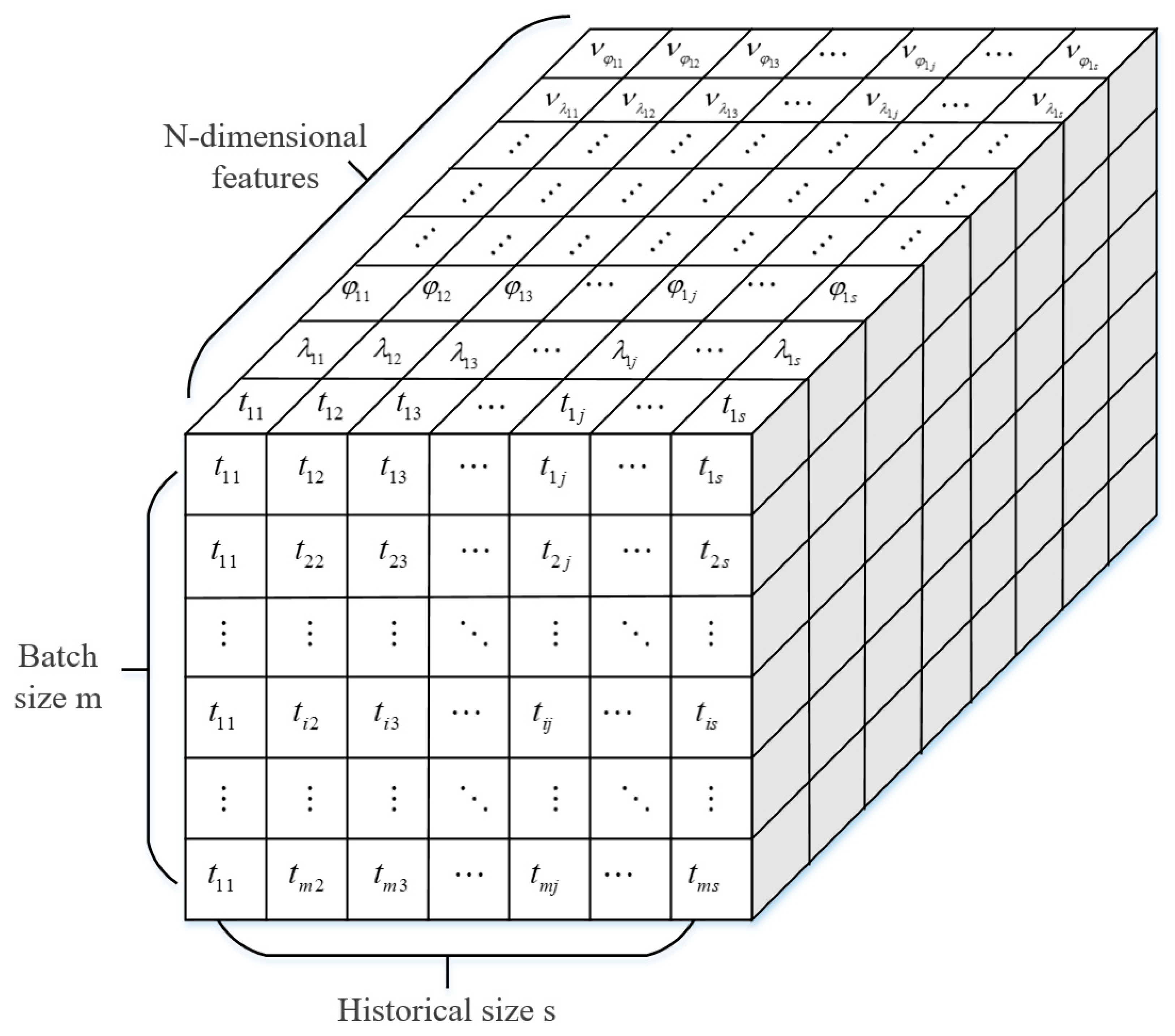
The input data structure of each training is shown in Figure 3. The size of the input data is m × s × N , where m is the batch size, namely the number of samples for each training. The size of each sample F i is 1 × s × N where s represents s historical moments, N represents the N-dimensional trajectory features and N = 15 . In Figure 3, 1 i m , 1 j s , where i represents the i th sample and j represents the j th moment.
In order to eliminate the effect of index scale, the input features of the model are normalized by dividing the maximum value, that is f i = f i / f i max , where f i is the i th feature, and f i max represents the maximum value of f i . The normalized matrix is used as the input of the model.
The true position at the s moment is denoted by Y = ( λ , φ ) . The label value ( p 1 , p 2 ) of the model output is calculated as Equation (15):
p 1 = λ 180 p 2 = φ 90
The actual output of the model is represented by ( y 1 , y 2 ) . Since the tanh activation function is used in the output layer of the network model, the final predicted position ( λ ^ , φ ^ ) is calculated as Equation (16):
λ ^ = 180 y 1 φ ^ = 90 y 2
The network model is trained to minimize the loss function, which includes mean square error and L2 regularization as Equation (17):
L o s s = 1 m i = 1 m y 1 i p 1 i 2 + y 2 i p 2 i 2 + c θ 2
where ( p 1 i , p 2 i ) represents the label value of the i th sample, and ( y 1 i , y 2 i ) represents the model output value of the i th sample. c is the regularization coefficient of weight parameters to avoid overfitting.
When the loss function decreases to convergence, the prediction model is accomplished, which can be used for real-time trajectory prediction. The overall process of position prediction based on deep learning is shown in Figure 4.

4. Experiments

In this section, we empirically evaluate our method. We first introduce the experimental conditions. Then, the experimental results and comparisons with other algorithms are presented.

4.1. Experimental Conditions

In this research, the position of the marine motion ship was collected by the space-based AIS system. AIS devices can be installed on vessels and shore-based stations, as well as space-based payloads of satellites. Shore-based AIS data are typically sampled at shorter intervals of the minute level, such as one minute, generally for inshore ships. Space-based AIS data are sampled at longer intervals limited to satellite orbital periods, typically at the hour level, and generally for far-shore ships. Since the observation time of the satellite is sparse and uneven, the input data, which are related to the observation time, are non-uniform in time. The time-scale requirements for trajectory prediction depend on the regression period of the satellites, and there are also unequal intervals.
The dataset selected for this experiment is the trajectory data of a single ship over a period of nearly a year around the east coast of the United States, with a total of about 6000 track points. Moreover, the time intervals of the track point are sparse and uneven, and about an hour. All trajectory samples are divided into the training set and test set at a ratio of 7:3. Different from the randomly generated training set and test set in other problems, in order to better conform to the scenario application and test the generalization of the model, the first 70% is selected as training sample data, and the 30% is the test sample data, which actually makes it harder to predict.
In data pre-processing, duplicate and abnormal data records are deleted. In this paper, a trajectory sequence containing s time is taken as an experimental sample, and the previous s - 1 moment data are used as available information to predict the position at the s th moment. Firstly, sample segmentation of historical trajectory data is carried out. Take the data of adjacent s moments as a sample. In this experiment, take s = 10 . It needs to be explained that if the value of the parameter s is too small, it cannot effectively represent the current moving status. Whereas if the value of s is too high, the correlation between the status of the ship’s predictive moment and the status of its starting moment becomes weaker, which will interfere with the prediction result. For the experimental samples in this paper, good experimental results were obtained when s = 10 was selected.
Then, the observation data of the first nine moments and the 10th observation time, which are given as available information, are exploited to compute the multi-dimensional trajectory feature matrix as Equation (13) in Section 3.1. The model can predict the positions at any given moment.
The prediction error of the model can be computed as Equation (18):
e λ = λ ^ λ e φ = φ ^ φ
where ( λ , φ ) represents the observation position, ( λ ^ , φ ^ ) indicating the predicted position. In order to evaluate the prediction result, the distance error is computed, which is expressed as the surface arc distance of the predicted position and the actual observed position. The calculation formula is expressed as Equation (19):
D i s = R arccos sin φ sin φ ^ + cos φ cos φ ^ cos ( λ ^ λ )
Root Mean Square Error (RMSE) is commonly used as the statistical criterion to evaluate model error, and the calculation formula is expressed as Equation (20):
R M S E λ = 1 n i = 1 n λ ^ i λ i 2 R M S E φ = 1 n i = 1 n φ ^ i φ i 2
In the problem of this paper, the prediction time is variable, and the error usually becomes larger with a longer prediction time. For the sake of unified measurement, the evaluation index of Relative Time Interval Mean Error (RTIME) is proposed. The calculation formula is expressed as Equation (21):
R T I M E λ = 1 n i 1 n λ ^ i λ i Δ t i 2 R T I M E φ = 1 n i 1 n φ ^ i φ i Δ t i 2 R T I M E D i s = 1 n i 1 n D i s i Δ t i 2
where n is the number of test samples, ( λ i , φ i ) and ( λ ^ i , φ ^ i ) are, respectively, the observation position and the prediction position of the i th sample, D i s i is the prediction distance error computed as Equation (19) of the i th sample, and Δ t i indicates the prediction interval of the i th sample in units of hours.

4.2. Experimental Results

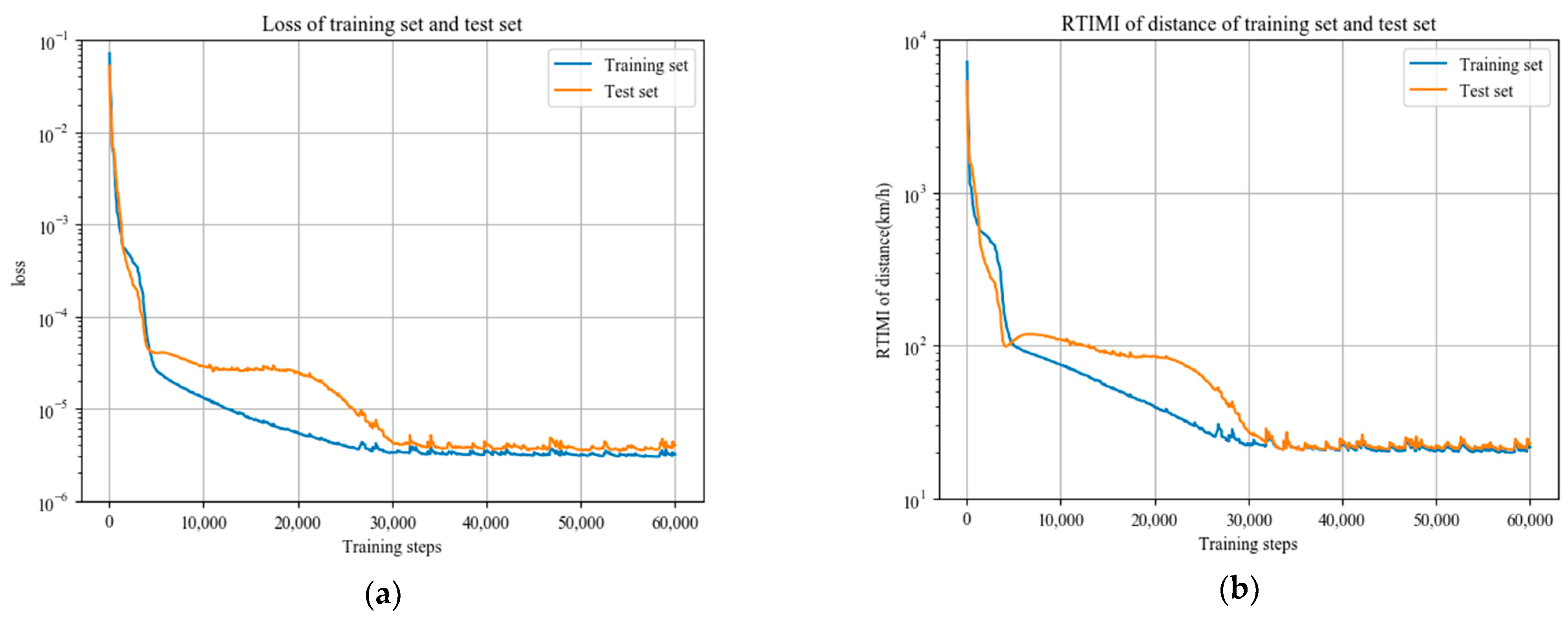
In order to intuitively show the accuracy improvement of the model during the training process, the prediction accuracy of the test set was synchronously tested during the training process. The model is implemented based on the TensorFlow [31] framework. The visualization function in the tensorboard of TensorFlow was used to visualize the changes in the loss function expressed as Equation (17) and R T I M E D i s expressed as Equation (21) during the training process. The training curves are shown in Figure 5. The value of the loss function of the training set and test sets during the training process are partially shown in Table 1. Through 60,000 training steps, the loss function of the training set gradually decreases to convergence and stability; the performance metrics of the test set is almost consistent with that of the training set, and there is no so-called overfitting problem in which the loss of the training set decreases while the loss of the test set rises.
Some of the predicted results of the test set on the well-trained model are shown in Table 2 below. Each row in the table is a sample record, including prediction duration, longitude error, latitude error, and distance error. In the last row, the statistical errors of all test samples are measured by RTIME expressed as Equation (21).
It can be seen from Table 2 that the prediction time is extremely uneven, which includes a short-term prediction of about 30 min and a long-term prediction of about 3 to 5 h. Using RTIME as a statistical evaluation indicator, the statistical errors are 0.157°, 0.118°, and 20.610°.
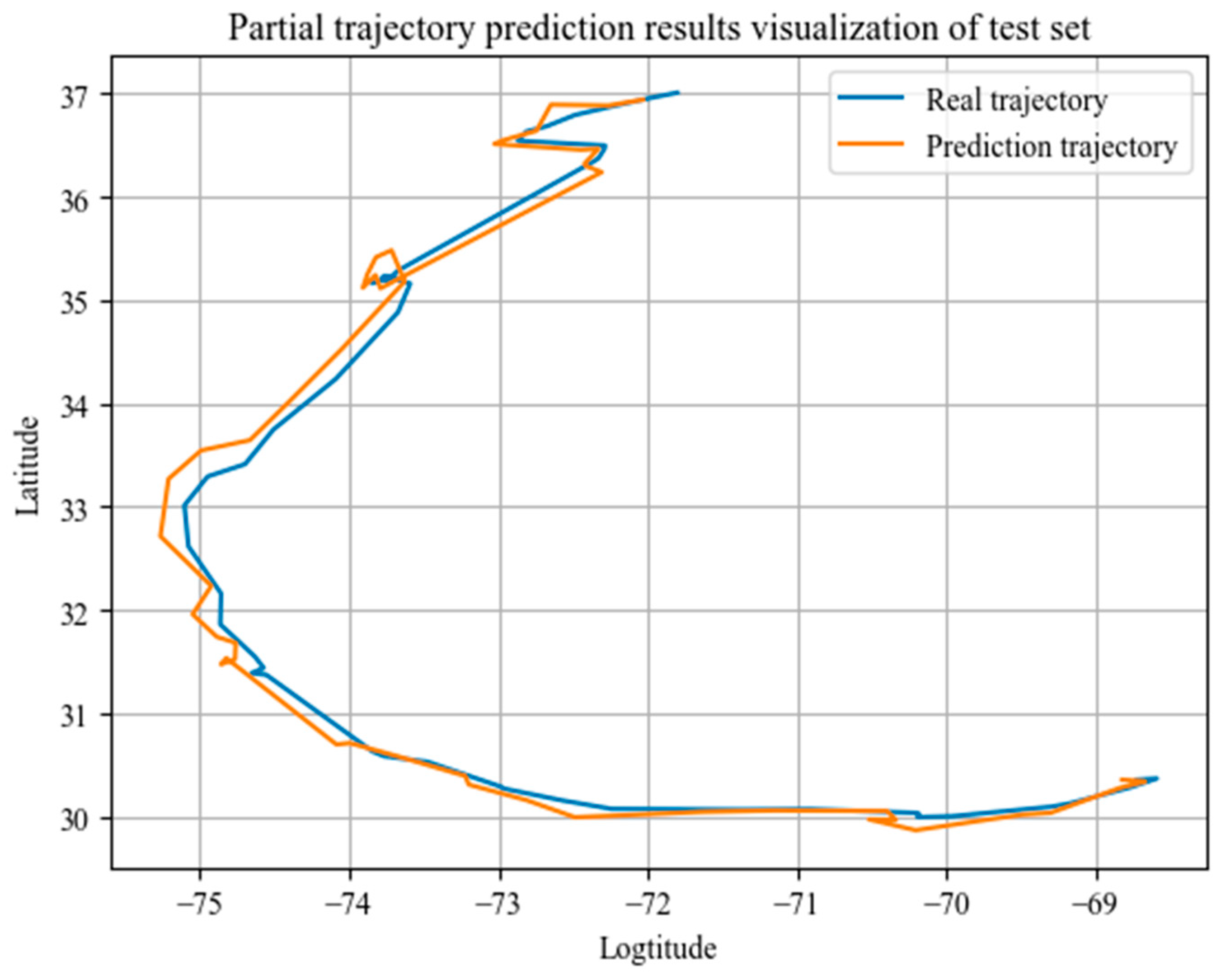
The trajectory predictions of the test set are partly visualized in Figure 6. It can be seen from the figure that the ship trajectory has strong nonlinear characteristics, and the prediction result can better grasp the movement direction. Furthermore, the deviation of the prediction result is relatively stable and has a relatively reliable prediction result.

4.3. Comparisons with Other Algorithms

To thoroughly test and analyze our proposed method, we run a series of experiments to compare our method with other algorithms, including the interpolation extrapolation method, fitting extrapolation method, grey prediction method, autoregressive prediction method, BP, and LSTM neural network model. The interpolation extrapolation method adopts cubic interpolation, which obtained the best results compared to nearest neighbor interpolation and linear interpolation. The fitting extrapolation method adopts polynomial fitting based on the least square method. The parametric experiment shows the best prediction results were obtained when the order of the polynomial is two. Grey prediction and autoregressive prediction methods are applied to data with consistent sampling intervals. Thus, polynomial interpolation and uniform sampling are first performed to obtain equal-interval data, and predictions of future fixed time intervals are then carried out. As the original trajectory data are non-stationary sequences, the autoregressive prediction method uses the Autoregressive Integrated Moving Average Model (ARIMA), which converts the non-stationary sequences to stationary sequences using the difference method, and the parameters are fine-tuned with the number of autoregressive terms p = 0, the order of differencing d = 1, and the number of moving average terms q = 2. The BP method is based on the multi-dimensional trajectory features presented in this paper. It adopts a three-layer network structure and is well-fitting after 10,000 training sessions. The LSTM method uses time as input and position as output; it is trained until the loss function no longer drops. All of these methods are parametrically optimized based on the dataset to ensure optimal results for the dataset studied in this paper. The RTIME expressed as Equation (21) is computed to measure the prediction performance. The experimental results of RTIME are shown in Table 3.
It can be seen from Table 3 that the prediction accuracy of this method is better than other methods. From the perspective of model accuracy and adaptability, the interpolation extrapolation method has inferior prediction accuracy. It can be concluded that the interpolation algorithm can only be used to complete the historical data under the constraint of both endpoints instead of predicting the extrapolation in the future. By contrast, fitting extrapolation can give better prediction accuracy. The grey and autoregressive prediction methods based on uniform sampling data have strict requirements for time series data. The experiments found that much of the trajectory sequence data cannot satisfy the requirements, so the method is not ideally applicable. Only the data satisfying the requirements are presented in Table 3. From the perspective of model complexity, interpolation, fitting, grey, and autoregressive models are simple and require fewer samples for prediction. However, since these models can only be used for short-term prediction, it needs to retrain a new model based on the data at previous moments; thus, these models have poor reusability. However, although the training process based on the historical data of this method is complicated, once the model is completed, it can be used repeatedly without the need to retrain and make predictions at any time.
In order to verify the rationality of multi-dimensional trajectory feature extraction in the input features of this paper, the comparison experiments of inputting only position features and of inputting multi-dimensional trajectory features are carried out based on the BP network model and CNN model. The experimental results are shown in Table 4.
As seen in Table 4, feature amplification by extracting multi-dimensional trajectory features can greatly improve prediction accuracy. Furthermore, the network model in this paper performs better than the BP network model.

5. Discussion

The algorithm experiments are introduced in detail in Section 3. The experimental conditions, including the experimental dataset, experimental procedure, and evaluation metrics, are presented, and then, the experimental results based on the experimental dataset are given. Through the analysis of the variation of the loss function in the training process, it was verified that the model is well-fitting without overfitting or underfitting problems. Some of the prediction results and the prediction trajectory curve are also shown. Furthermore, comparison experiments of different algorithms were carried out. Based on the above experimental process, we present an extensive discussion of experimental results as follows.
First, according to the prediction results presented in Table 2, overall, the longer the forecast, the greater the prediction error, which is consistent with our view that the longer the forecast, the greater the location uncertainty and the more complex the forecast. However, there were a few opposite cases, that is, in which the prediction error was instead more prominent for shorter prediction durations. Through the tracking of the prediction sample data, it was found that the larger errors mainly occurred in the ship steering stage, that is, when the prediction moment is in the ship turning phase, it increases the prediction difficulty, and thus, the prediction error is more prominent. In addition, the prediction errors are smaller when the ship is on a smooth sail. This can be seen in Figure 6. The method extracts extensive motion features from raw trajectory data. However, ship steering is a change in motion state that cannot be inferred simply from motion features, and the reasons for the sudden turning of ships are usually complicated. How to combine more factors, such as meteorological data and geographic data, to make predictions and thus improve prediction accuracy for complex scenarios such as steering, is a problem that, in order to be resolved, requires further research.
In addition, through the comparison experiments of different algorithms in Table 3, with the analysis of experimental results reported in related works, we can conclude that the comprehensive performance of neural network algorithms such as CNN and BP is better than that of statistical algorithms such as fitting extrapolation and autoregressive when applied to the track prediction problem. For the LSTM neural network, it is applicable to processing temporal series data because of its ability of long and short-term memory. The LSTM neural network with the design of time as input and position as output is adopted in the comparison experiment but does not realize better results. This may be related to the design architecture of the LSTM model and its training strategy. Simple strategies that consider trajectory as three-dimensional record sequences (time, latitude, longitude) may lead to the hard convergence of LSTM models for complex navigation patterns learning. The CNN network in this paper, on the other hand, achieves the purpose of temporal correlation learning through its local correlation and weight-sharing properties and obtains a better-fitting effect.
According to Table 4, we analyzed the effects of different input features on prediction accuracy using both BP and CNN network structures. Differentiated results are achieved for the same network model structure, differing only in input features. When augmented multi-dimensional feature information such as position, velocity, and acceleration as inputs, the model achieved better prediction results than when only inputting three-dimensional features (time, longitude, and latitude). Therefore, the richness of the input features helps to improve the predicted accuracy.
In general, the CNN model designed in this paper achieves superior prediction performance for sparse trajectory data. However, it also provokes reflection and indicates directions for future research. It is of great significance to extend relevant features as inputs for better prediction, and combining multi-factor features to achieve track prediction for complex behavioral scenarios such as steering is needed for further research.

6. Conclusions

In this paper, a trajectory prediction model based on multi-dimensional trajectory features and a CNN model structure is proposed aimed at the characteristics of space-based observation data, which can process sparse and long non-uniform time series trajectory data without an interpolation algorithm for uniform sampling and is adaptive to prediction requirements of hour-scale variable time intervals.
Because of the correlation of ship movement state in the time domain, based on the local correlation perception and weight-sharing characteristics of CNN, this paper innovatively applies the CNN model to the trajectory prediction problem. In order to exploit the ship’s motion characteristics to the greatest extent from the raw trajectory data, multi-dimensional features extraction is carried out to construct the multi-dimensional trajectory feature matrix as the input of the network model, and the time–space correlation characteristic of the track data is representant and mined. To the best of our knowledge, this is the first study in which local connection characteristics of the CNN have been applied to the time domain to solve ship trajectory prediction problems. By carrying out experiment and method comparison, it shows that the method can achieve better prediction accuracy and adaptability for the sparse non-uniform trajectory data.
Research on the trajectory prediction of maritime moving targets for satellite resource scheduling is of great application value; one of the difficulties is the uncertainty of maritime moving targets. The trajectory prediction algorithm can decrease the uncertainty of maritime moving targets in order to reduce the blind search when making the satellite search plan, guide the satellite observation of the target, and greatly improve the efficiency of target search.

7. Limitation of the Study

In this paper, a method is presented for sparse trajectory data with long non-uniform time series intervals. Experiments show that better prediction results can be obtained for the requirement of long and non-equidistant prediction duration on the hourly scale. The limitation of this method is that this method does not necessarily show better prediction performance for minute-scale dense time series trajectory data. In addition, since the method is based on deep learning method, the distribution of test samples should be consistent with the training samples. Otherwise, the accuracy of prediction may be affected. Despite some research progress, effective and reliable trajectory prediction remains challenging, as marine navigation is a complex system of stochastic time variations.

8. Future Recommendations

In future research work, we need to further model optimization and performance enhancement for complex scenarios such as ship steering. We will consider classifying the different navigation patterns of moving targets and separately train track samples of different patterns in order to build precise prediction models. On the other hand, the prediction model can be further improved by incorporating more relevant constraints such as potential navigation areas, geographical conditions, and even meteorology.

Author Contributions

Conceptualization, X.P. and J.Z.; methodology, X.Z. and J.Z.; software, X.Z. and X.W.; validation, X.W. and X.P.; formal analysis, X.Z.; investigation, X.Z. and X.W.; resources, X.P. and J.Z.; data curation, X.Z.; writing—original draft preparation, X.Z.; writing—review and editing, X.P., J.Z. and X.W. All authors have read and agreed to the published version of the manuscript.

Funding

This research received no external funding.

Institutional Review Board Statement

Not applicable.

Informed Consent Statement

Not applicable.

Data Availability Statement

The data used to support the findings of this study are available from the corresponding author upon request.

Conflicts of Interest

The authors declare no conflict of interest.

References

  1. Ci, Y.Z.; He, R.J.; Xu, Y.F.; Tan, Y.J. Method of target motion prediction for moving target search by satellite. Control. Decis. 2009, 24, 1007–1012. [Google Scholar]
  2. Chen, C.-C.; Chiang, M.-F.; Peng, W.-C. Mining and clustering mobility evolution patterns from social media for urban informatics. Knowl. Inf. Syst. 2015, 47, 381–403. [Google Scholar] [CrossRef]
  3. Zhang, C.; Han, J.; Shou, L.; Lu, J.; La Porta, T. Splitter: Mining fine-grained sequential patterns in semantic trajectories. Proc. VLDB Endow. 2014, 7, 769–780. [Google Scholar] [CrossRef]
  4. Zheng, Y. Trajectory data mining: An overview. ACM Trans. Intell. Syst. Technol. 2015, 6, 1–41. [Google Scholar] [CrossRef]
  5. Yao, D.; Zhang, C.; Zhu, Z.; Huang, J.; Bi, J. Trajectory Clustering via Deep Representation Learning. In Proceedings of the 2017 International Joint Conference on Neural Networks (IJCNN), Anchorage, AL, USA, 14–19 May 2017; pp. 3880–3887. [Google Scholar]
  6. Zhang, J.; Shi, H.; Cui, L. Location prediction model based on transportation mode and semantic trajectory. J. Comput. Res. Dev. 2019, 56, 1357–1369. [Google Scholar]
  7. Xie, G.; Shangguan, A.; Fei, R.; Ji, W.; Ma, W.; Hei, X. Motion trajectory prediction based on a CNN-LSTM sequential model. Sci. China Inf. Sci. 2020, 63, 1–21. [Google Scholar] [CrossRef]
  8. Tang, H.; Yin, Y.; Shen, H. A model for vessel trajectory prediction based on long short-term memory neural network. J. Mar. Eng. Technol. 2019, 21, 136–145. [Google Scholar] [CrossRef]
  9. Xu, Y.F.; Tan, Y.J.; He, R.J.; Ci, Y.Z. Multi-model Prediction for Maritime Moving Target Motion. Huoli Yu Zhihui Kongzhi 2012, 37, 20–25. [Google Scholar]
  10. Capobianco, S.; Millefiori, L.M.; Forti, N.; Braca, P.; Willett, P. Deep Learning Methods for Vessel Trajectory Prediction Based on Recurrent Neural Networks. IEEE Trans. Aerosp. Electron. Syst. 2021, 57, 4329–4346. [Google Scholar] [CrossRef]
  11. Li, M.; Lv, B.; Dong, W.; Wang, D. Model of multi-Sensor Data Fusion and Trajectory Prediction Based on Echo State Network. In Proceedings of the 2010 International Conference on Computer, Mechatronics, Control and Electronic Engineering, Changchun, China, 24–26 August 2010; pp. 338–341. [Google Scholar]
  12. Bogaerts, T.; Masegosa, A.D.; Angarita-Zapata, J.S.; Onieva, E.; Hellinckx, P. A graph CNN-LSTM neural network for short and long-term traffic forecasting based on trajectory data. Transp. Res. Part C Emerg. Technol. 2020, 112, 62–77. [Google Scholar] [CrossRef]
  13. Neto, J.B.P.; Mitton, N.; Campista, M.E.M.; Costa, L.H.M. Dead reckoning using time series regression models. In Proceedings of the 4th ACM MobiHoc Workshop on Experiences with the Design and Implementation of Smart Objects, Los Angeles, CA, USA, 25 June 2018; pp. 1–6. [Google Scholar]
  14. Rong, H.; Teixeira, A.; Soares, C.G. Ship trajectory uncertainty prediction based on a Gaussian Process model. Ocean Eng. 2019, 182, 499–511. [Google Scholar] [CrossRef]
  15. Liu, J.; Shi, G.; Zhu, K. Vessel Trajectory Prediction Model Based on AIS Sensor Data and Adaptive Chaos Differential Evolution Support Vector Regression (ACDE-SVR). Appl. Sci. 2019, 9, 2983. [Google Scholar] [CrossRef] [Green Version]
  16. Zhou, H.; Chen, Y.; Zhang, S. Ship Trajectory Prediction Based on BP Neural Network. J. Artif. Intell. 2019, 1, 29–36. [Google Scholar] [CrossRef]
  17. Zou, J.; Chen, S.; Cheng, Z.; Liao, J. Research on Collision Avoidance of Navigation Marks Based on Neural Network. In Proceedings of the 2020 7th International Forum on Electrical Engineering and Automation (IFEEA), Hefei, China, 25–27 September 2020; pp. 632–635. [Google Scholar]
  18. Suo, Y.; Chen, W.; Claramunt, C.; Yang, S. A Ship Trajectory Prediction Framework Based on a Recurrent Neural Network. Sensors 2020, 20, 5133. [Google Scholar] [CrossRef]
  19. Park, J.; Jeong, J.; Park, Y. Ship Trajectory Prediction Based on Bi-LSTM Using Spectral-Clustered AIS Data. J. Mar. Sci. Eng. 2021, 9, 1037. [Google Scholar] [CrossRef]
  20. Gao, D.-W.; Zhu, Y.-S.; Zhang, J.-F.; He, Y.-K.; Yan, K.; Yan, B.-R. A novel MP-LSTM method for ship trajectory prediction based on AIS data. Ocean Eng. 2021, 228, 108956. [Google Scholar] [CrossRef]
  21. Zhao, J.; Lu, J.; Chen, X.; Yan, Z.; Yan, Y.; Sun, Y. High-fidelity data supported ship trajectory prediction via an ensemble machine learning framework. Phys. A Stat. Mech. Appl. 2021, 586, 126470. [Google Scholar] [CrossRef]
  22. Elnagar, A.; Gupta, K. Motion prediction of moving objects based on autoregressive model. IEEE Trans. Syst. Man Cybern. 1998, 28, 803–810. [Google Scholar] [CrossRef]
  23. LeCun, Y.; Bengio, Y.; Hinton, G. Deep learning. Nature 2015, 521, 436–444. [Google Scholar] [CrossRef]
  24. Zhang, Q.; Yang, L.T.; Chen, Z. Deep computation model for unsupervised feature learning on big data. IEEE Trans. Serv. Comput. 2015, 9, 161–171. [Google Scholar] [CrossRef]
  25. Cordts, M.; Omran, M.; Ramos, S.; Rehfeld, T.; Enzweiler, M.; Benenson, R.; Franke, U.; Roth, S.; Schiele, B. The cityscapes dataset for semantic urban scene understanding. In Proceedings of the IEEE Conference on Computer Vision and Pattern Recognition, Las Vegas, NV, USA, 27–30 June 2016; pp. 3213–3223. [Google Scholar]
  26. Silver, D.; Huang, A.; Maddison, C.J.; Guez, A.; Sifre, L.; van den Driessche, G.; Schrittwieser, J.; Antonoglou, I.; Panneershelvam, V.; Lanctot, M.; et al. Mastering the game of Go with deep neural networks and tree search. Nature 2016, 529, 484–489. [Google Scholar] [CrossRef] [PubMed]
  27. Litjens, G.; Kooi, T.; Bejnordi, B.E.; Setio, A.A.A.; Ciompi, F.; Ghafoorian, M.; van der Laak, J.A.; Van Ginneken, B.; Sánchez, C.I. A survey on deep learning in medical image analysis. Med. Image Anal. 2017, 42, 60–88. [Google Scholar] [CrossRef] [PubMed] [Green Version]
  28. Lecun, Y.; Bottou, L.; Bengio, Y.; Haffner, P. Gradient-based learning applied to document recognition. Proc. IEEE 1998, 86, 2278–2324. [Google Scholar] [CrossRef]
  29. Jeong, H.; Park, S.; Woo, S.; Lee, S. Rotating Machinery Diagnostics Using Deep Learning on Orbit Plot Images. Procedia Manuf. 2016, 5, 1107–1118. [Google Scholar] [CrossRef]
  30. Simonyan, K.; Zisserman, A. Very deep convolutional networks for large-scale image recognition. arXiv 2014, arXiv:1409.1556. [Google Scholar]
  31. Abadi, M.; Barham, P.; Chen, J.; Chen, Z.; Davis, A.; Dean, J.; Devin, M.; Ghemawat, S.; Irving, G.; Isard, M. {TensorFlow}: A system for {Large-Scale} machine learning. In Proceedings of the 12th USENIX Symposium on Operating Systems Design and Implementation (OSDI 16), Savannah, GA, USA, 2–4 November 2016; pp. 265–283. [Google Scholar]
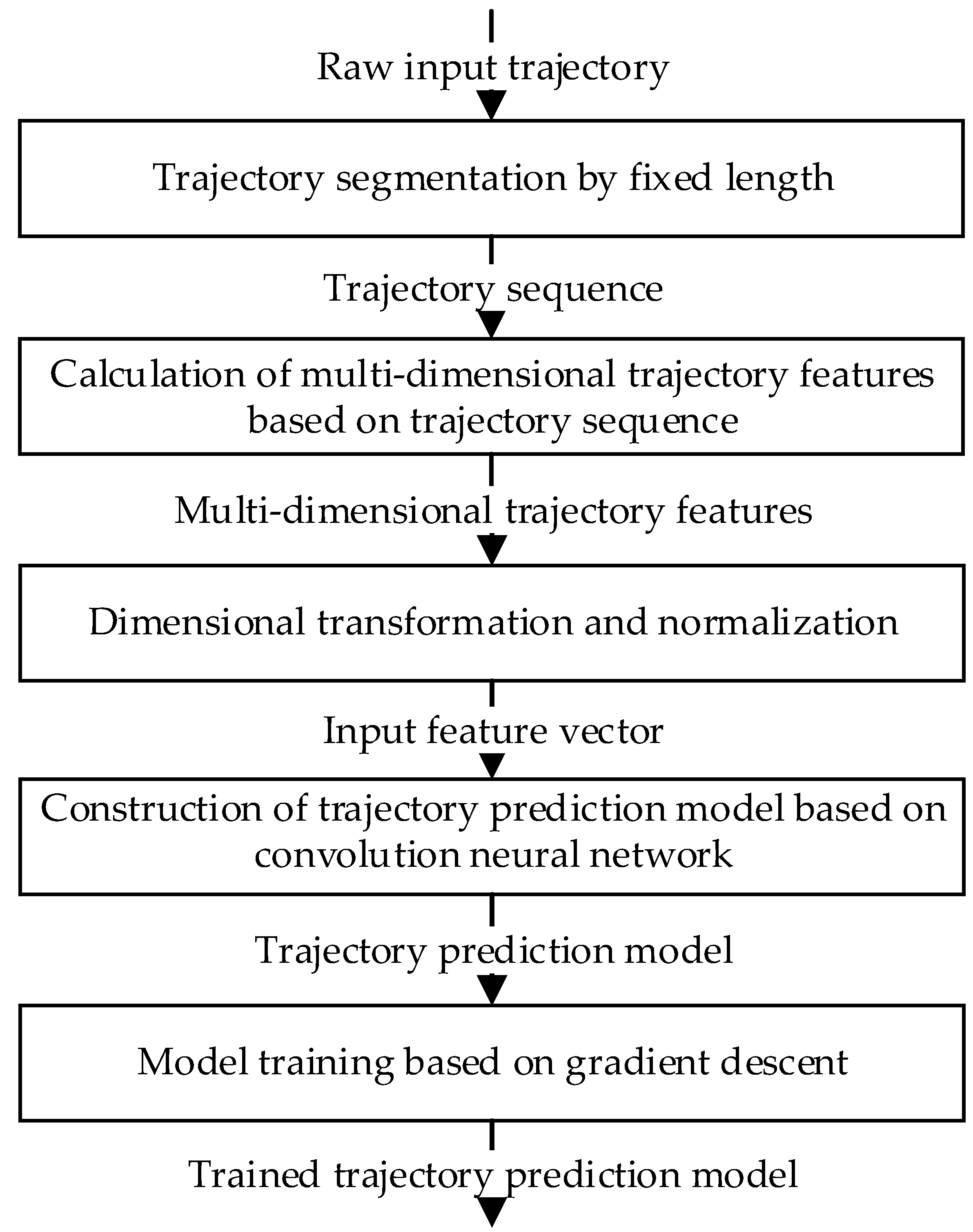
Figure 1. The overall flowchart of the method.
Applsci 12 11905 g001
Figure 2. The architecture of the network.
Applsci 12 11905 g002
Figure 3. The input structure of the CNN prediction model.
Applsci 12 11905 g003
Figure 4. Diagram of the Training and Testing Process of the Trajectory Prediction Model.
Applsci 12 11905 g004
Figure 5. Training curves: (a) the loss function variation curve of the training set and test set; (b) the R T I M E D i s variation curve of the training set and test set.
Applsci 12 11905 g005
Figure 6. Visualization of trajectory predictions. The horizontal axis is longitude, and the vertical axis is latitude. In addition, the blue curve is the real trajectory, and the orange curve is the prediction trajectory.
Applsci 12 11905 g006
Table 1. Performance metrics of the training set and test set in the training process.
Training StepsLoss of Training SetLoss of Test Set
10.2393510.217599
20004.55702 × 10−42.79363 × 10⁻⁴
40003.19982 × 10−53.81833 × 10⁻⁵
60002.06495 × 10−53.98102 × 10⁻⁵
80001.58536 × 10−53.26941 × 10⁻⁵
10,0001.25557 × 10−52.85061 × 10⁻⁵
20,0005.28681 × 10−62.37062 × 10⁻⁵
30,0003.27563 × 10−64.25452 × 10⁻⁶
40,0003.11066 × 10−63.63867 × 10⁻⁶
50,0003.06778 × 10−64.76017 × 10⁻⁶
60,0003.14196 × 10−63.81424 × 10⁻⁶
Table 2. The predicted results of the test set.
NumberPrediction
Duration (h)
Longitude
Error (Degree)
Latitude
Error (Degree)
Distance
Error (km)
10.305−0.08594−0.009159.06339
20.677−0.193−0.26936.207
30.854−0.071−0.11815.112
41.202−0.221−0.24435.721
51.362−0.191−0.04220.232
61.8120.1020.00610.439
72.11250.0965−0.326437.6564
82.1130.0222491−0.3699141.1962
92.1450.2130.02722.082
102.172780.259359−0.3072643.6366
112.219440.33176−0.3870455.324
123.664−0.202414−0.1241825.3107
133.79528−0.321965−0.5351468.1318
143.90556−0.0867181−0.42876848.5071
155.866−0.2643−0.40352.395
…………………………
RTIME 0.1570.11820.610
Table 3. Performance comparison with other algorithms.
Algorithm R T I M E λ
(Degree/h)
R T I M E φ
(Degree/h)
R T I M E Dis
(km/h)
interpolation extrapolation [11]3.25473.7510340.0171
fitting extrapolation0.27770.213936.4040
grey prediction [9]0.26250.208425.1501
autoregressive prediction [22]0.27440.261541.98
BP neural network [16]0.3050.12732.513
LSTM neural network [8]1.0180.536119.306
the algorithm presented in this paper0.1570.11820.610
Table 4. Performance comparison with other solutions.
Solution R T I M E λ
(Degree/h)
R T I M E φ
(Degree/h)
R T I M E Dis
(km/h)
BP network with only position features [16]0.3450.14641.654
BP network with multi-dimensional trajectory features [16]0.3050.12732.513
CNN with only position features0.1890.16128.777
the solution presented in this paper0.1570.11820.610
Publisher’s Note: MDPI stays neutral with regard to jurisdictional claims in published maps and institutional affiliations.