Modeling and HDA-CR Solution of Multi-Period Allocation Scheme of Hazardous Materials under Uncertainty

Featured Application

In this study, an improved multi-objective difference evolution algorithm (HDA-CR) is proposed and applied to the formulation of a multi-period allocation scheme for hazardous materials under uncertainty, which can provide a reference for solving similar large-scale multi-dimensional assignment problems.

Abstract

Developing a multi-period allocation scheme for life-limited hazardous materials is essential to ensure safe and sustainable hazardous material management. In this study, the allocation risk under uncertainty is measured by a type-II fuzzy number, and a bilevel chance constrained programming model is established with the minimum cumulative number of reserve points participating in allocation and the minimum cumulative allocation risk as to the objective functions. Aiming at the multi-dimensional characteristics of multi-period, multi-reserve points, multi-consumption points, and multi-hazardous materials types, and the resource conflict problem in the allocation scheme formulation process, a multi-objective hierarchical differential evolution algorithm with coding repair strategy was designed. By comparing with the classical multi-objective optimization algorithm, the algorithm can search for a more excellent Pareto solution set at the expense of certain time complexity. At the same time, when the decision-maker’s preference is introduced, the method can select a more appropriate multi-period allocation scheme from the perspective of the overall situation and the decision-maker. It provides a reference for determining the rational allocation scheme of resources under the long-term allocation of hazardous materials.

1. Introduction

With the continuous development of the industrial level and productivity of the society, the types and the market demand are also increasing in hazardous materials. For some special hazardous materials with storage life limitation, such as weapons and ammunition, nuclear materials, and hazardous chemicals, a certain quantity of hazardous materials with less remaining storage life needs to be regularly allocated from the reserve warehouse to the designated location for use. How to reduce the allocation risk of specific hazardous materials while ensuring the multiple demands of industry, military and energy, and how to use new solutions to deal with chemical, biological, radiological, and nuclear threats brought by hazardous materials allocation to achieve sustainable development remains to be studied [1].

In practical application, the reserve warehouse mainly determines the allocation scheme according to the demand for various types of hazardous materials in the next period and the remaining storage life of the hazardous materials to which it belongs; however, it lacks multiple periods of a hazardous materials allocation scheme. However, the differences in such factors as the geographical location and inventory of the warehouses of reserve hazardous materials, the location of the demand points, and the hazardous materials demand of each period cause the phenomenon of unreasonable resource allocation of hazardous material in the subsequent allocation process, resulting in the phenomenon of more remaining reserve life in the hazardous materials used in the allocation and some hazardous materials being scrapped due to their service exceeding the storage time limit. Therefore, it is especially important to coordinate the hazardous materials inventory in different places and formulate sustainable multi-periods of allocation scheme in advance.

This work aims to study the method of developing the optimal sustainable multi-period allocation scheme for a class of hazardous materials that need to be distributed regularly under uncertainty. On the premise of determining the location and transportation path of each reserve point and consumption point, we must fully consider the risk uncertainty factors in the allocation process of hazardous materials, use type-II fuzzy numbers to measure the unit allocation risk, and establish a bilevel chance constraint programming model for multi-period allocation of hazardous materials. According to the characteristics of the problem, a new hierarchical differential evolution algorithm with coding repair strategy (HDA-CR) is designed, which can provide an algorithm reference for solving multi-dimensional complex hazardous material assignment problems. Finally, the effectiveness of the algorithm is verified through comparative experiments.

The rest of this paper is stated as follows. First, Section 2 summarizes the literature research about hazardous material allocation. The description of hazardous materials allocation risk model and multi-period allocation model is shown in Section 3. Section 4 describes the proposed HDA-CR. Section 5 provides some numerical experiments to test the proposed algorithm. Finally, the work is summarized in Section 6. The overall research framework is shown in Figure 1.

2. Research Overview

At present, the research on hazardous material allocation mainly focuses on the path optimization and risk assessment. In the aspect of path optimization, Izdebski proposed a minimization model considering the probability of hazardous materials transport accidents, on which the ant colony and genetic algorithm are used to determine the hazardous materials transport route [2]; Zografos designed a heuristic algorithm to solve the scheduling problem of hazardous materials, and defined a double-objective scheduling model with minimum risk and minimum cost [3]. Li designed a novel optimization model of a multimodal hub-and-spoke network with a detour (MHSNWD) for hazardous materials on the strategic level, considering the dual goals of risk and cost management of hazardous materials transportation [4]. However, for some specific hazardous materials, cost is not the most important factor to be considered. For example, Saat carried out the research on the safety design optimization of the generalized railway tank car for the transportation of hazardous materials from the perspective of transportation efficiency and safety [5]. Therefore, how to meet the demand for use and ensure sustainable resource allocation under the premise of safety is the most important issue to consider.

In terms of risk assessment, Liu analyzed the different factors affecting accidents in different populations and environments, and presented a risk assessment model of hazardous materials road transportation under time-varying conditions by considering the bearing capacity of the assessed area [6]. Korytárová monitored the frequency of individual risk factors in qualitative risk analysis, and used a Monte Carlo approach to test the interaction of the impact of key variables on project efficiency [7]. Park proposed a model for real-time prediction of accident consequences for dynamic risk assessment of LNG fuel supply system rooms [8]; Krejci provided a series of risk assessment methods for hazardous material transportation, such as the expert consultation method, fault-tree analysis, failure mode impact and cause analysis, and reliability assessment [9]. Verter presented a methodology for assessment of the hazardous materials transport risk in a multicommodity, multiple origin-destination setting, which was integrated with a Geographical Information System (GIS) and made large-scale implementation possible [10]. Topuz used the analytic hierarchy process and fuzzy logic to integrate the environment and human health into the risk assessment of hazardous materials in order to support environmental decision-makers with quantitative and directive results [11].

Due to the lack of consistent and sufficient hazardous material transportation accident data, it is usually difficult to obtain the parameters required for accurate transportation risk measurement during actual hazardous materials allocation. Different allocation risk measurement methods will lead to different decision-making results [12]. Many studies show that the high uncertainty of allocation risk significantly affects the decision making of hazardous materials allocation [13,14]. Therefore, the allocation decisions obtained in a deterministic environment may have difficulty meeting the actual needs of mobile hazardous material risk management.

Risk modeling of hazardous material under uncertainty received extensive attention. Du assumed that the path length in the traffic network is a fuzzy variable, and proposed a fuzzy multi-objective programming model to minimize transportation risk, time, and fuel consumption, and build a chance constraint model based on the fuzzy credibility theory [15]. Zero used fuzzy random theory to balance the lowest cost and the lowest risk, and solved the problem of gas station positioning [16]. Yan established a transport vehicle scheduling model considering random interference and travel time [17]. Ljubojevic used an adaptive neuro-fuzzy inference system to investigate the cost and risk assessment of multi-objective routing of hazardous materials transport on urban road networks and tested it in a case study of oil and oil derivatives allocation in Belgrade, Serbia [18]. Berglund studied the impact of uncertainty and the robust optimization problem of hazardous material transportation [19].

The multi-period allocation scheme of hazardous material studied in this paper belongs to a kind of optimization problem involving multiple objective functions, multiple reserve points, multiple consumption points, multiple types of hazardous materials, and multiple periods. Its decision space is huge, and it is often difficult to solve the problem by enumerating. In solving this kind of optimization model, various heuristic algorithms received extensive attention [20,21,22]. For example, in research of road screening issues of hazardous materials transportation, Ma built a road screening algorithm of hazardous materials transportation based on genetic algorithms and the Levenberg Marquardt neural network (GA-LM-NN) by analyzing 15 attribute data of each road network section [23]. Bula used variable neighborhood search to solve the vehicle routing problem for hazardous materials transportation [24]. Zero proposed two algorithms to the bi-objective shortest path problem for the road transport of hazardous materials, including the first one, using a modified Gandibleux revision of Martin’s algorithm and the second one based on the A* algorithm acceleration technique [25].

3. Problem Description and Modeling

3.1. Problem Description

This type of hazardous materials allocation problem can be defined as a complex large-scale assignment problem under uncertainty, assuming that there are $n$ hazardous materials reserve points in a region with a total of $K$ different hazardous material types. In each period $t\in \{1,2,\dots ,T\}$, all kinds of hazardous materials need to be allocated to the hazardous materials consumption points to meet the needs $c_{tj}{}^k$ of each consumption point in that period, and there are $m$ consumption points. On the basis of considering the hazardous materials inventory near the rated life of the existing reserve points, the allocation scheme $X=(X_1,X_2,\dots ,X_T)$ of multi-periods, multi-reserve points, multi-consumption points, and multi-hazardous material types is prepared for such hazardous materials. The model parameters are described in

Table 1. Model parameter setting.

Parameters	Parameter Significance
$a_i$	The $i$th reserve point
$d_j$	The $j$th consumption point
$y_i^k$	Initial reserve quantity of hazardous materials of type $k$ at $a_i$
${\epsilon }_{ti}^k$	Remaining reserve quantity of hazardous materials of type $k$ at $a_i$ after period $t$
$c_{tj}{}^k$	Demand for hazardous materials of type $k$ at $d_j$ in period $t$
$l_{ij}$	Generalized distance between $a_i$ and $d_j$
$x_{tij}^k$	Decision variables, quantity of hazardous materials of type $k$ allocated from $a_i$ to $d_j$ in period $t$
$r_{ij}$	Population density on the section from $a_i$ to $d_j$
$p{j}_{ij}$	Vehicle traffic accidents on the section from $a_i$ to $d_j$
$s_k$	Accident impact range of hazardous materials of type $k$
${\theta }_R$	Risk threshold
$f$	Cumulative allocation risk
$g$	Cumulative quantity of reserve points performing the allocation task
${\alpha }^u,{\alpha }^l$	degree of confidence

.

3.2. Problem Assumptions

Assumption 1.

The inventory of hazardous material at each reserve point that is eligible for allocation with a remaining life below a specific standard will not increase during the allocation.

Assumption 2.

The positions of reserve points and consumption points are known and fixed, and their transportation distances are known.

Assumption 3.

The demand for all types of hazardous materials at consumption points in each period is known.

Assumption 4.

Road transportation is considered as the only allocation mode of hazardous materials.

3.3. Allocation Risk Model

The allocation risk of hazardous materials can usually be measured in combination with the probability and consequence of hazardous accidents [26], which is given as follows:

$$f_{tij}=P_{ij}\times C_{tij}, t=1,2,\dots ,T, i=1,2,\dots ,n, j=1,2,\dots ,m$$

(1)

where, $f_{tij}$ is the allocation risk from $a_i$ to $d_j$ in period $t$, considering the transportation risk. $P_{ij}$ is the transportation accident probability on the road section from $a_i$ to $d_j$, and $C_{tij}$ is the accident consequence on the road section from $a_i$ to $d_j$ in period $t$.

Referring to the risk modeling approach proposed by Errkut [27] for transporting hazardous materials, the allocation risk described above can be defined as:

$$f_{tij}=p{j}_{ij}\times l_{ij}\times p{d}_{ij}\times {\displaystyle \sum _{k=1}^K(s_k\times x_{tij}{}^k)}$$

(2)

where $P_{ij}=p{j}_{ij}\times l_{ij}$ is used to measure the transportation accident probability on the road section from $a_i$ to $d_j$, which is measured by the probability of traffic accidents $p{j}_{ij}$ and the length $l_{ij}$ on this road section, and $C_{tij}=p{d}_{ij}\times {\displaystyle \sum _{k=1}^K(s_k\times x_{tij}{}^k)}$ is used to measure the accident consequences of this allocation. The hazard range and surrounding population density are used to measure the severity of accidents when hazardous accidents occur. However, the traffic accident probability, population density, and accident impact range that determine the allocation risk are difficult to accurately measure. How to quantitatively describe these uncertain factors determines the allocation risk value at each period.

3.3.1. The Traffic Accident Probability

Considering the lack of data on the occurrence of accidents involving hazardous materials transport vehicles on the corresponding road sections, the accident probability for measuring the allocation risk can refer to the vehicle traffic accidents on the road sections. The historical interval frequency is used to describe the probability of traffic accidents for hazardous materials in the future allocation periods, i.e., $p{j}_{ij}=[p{j}_{ij}^l,p{j}_{ij}^u]$, where $p{j}_{ij}^l$ and $p{j}_{ij}^u$ refer to the minimum and maximum frequency of traffic accidents on the road section from $a_i$ to $d_j$ in the statistical period.

3.3.2. Population Density

Due to the differences of mobility and regional distribution of the population, the population density on the accident road section cannot be accurately predicted. In order to simplify the analysis, the population density on the accident roadway section is equated to the average population density on this roadway section. According to the results of the latest census, the population density on the allocation road section is described by the number of intervals, i.e., $p{d}_{ij}=[p{d}_{ij}^l,p{d}_{ij}^u]$, where $p{d}_{ij}^l$ and $p{d}_{ij}^u$ are the minimum and maximum average population density on the road section from $a_i$ to $d_j$.

3.3.3. Accident Impact Range

Different types of hazardous materials have different levels of hazard in the event of an accident. For example, the explosion range of explosion-prone hazardous materials can be used to measure the accident impact range. If the explosion range of allocated hazardous materials is large, the hazard range of the accident is large, and the explosion range is small, the hazard range of the accident is relatively small. However, it is difficult to estimate the specific type, quantity, and impact range of the superimposed explosion of hazardous materials when the accident occurs. Therefore, fuzzy numbers can be used to measure the hazard range of the accident of allocated hazardous materials, i.e., $[s^l,s^u]\times {\displaystyle \sum _k^K{x}_{tij}^k}={\displaystyle \sum _k^K{s}_k\times x_{tij}^k}$, where $s^l$ and $s^u$ are, respectively, the minimum and maximum accident impact range in all types of hazardous materials.

3.3.4. Allocation Risk Measures

It can be seen from the above analysis that the allocation risk of hazardous materials allocated from $a_i$ to $d_j$ in period $t$ can be expressed as:

$${\tilde{f}}_{tij}=[p{j}_{ij}^l,p{j}_{ij}^u]\times l_{ij}\times [p{d}_{ij}^l,p{d}_{ij}^u]\times [s^l,s^u]\times {\displaystyle \sum _{k=1}^K{x}_{tij}{}^k}$$

(3)

According to the multiplication rules of interval numbers, the multiplication of any two interval numbers $[a b]$ and $[c d]$ yields:

$$[a,b]\times [c,d]=[\min (ac,ad,bc,bd),\max (ac,ad,bc,bd)]$$

(4)

where $\min (ac,ad,bc,bd)$ and $\max (ac,ad,bc,bd)$ are, respectively, the minimum and maximum values of the resulting four interval boundary combinations $ac$, $ad$, $bc$ and $bd$.

This multiplication operation preserves the uncertainty information of the fuzzy variables by enlarging the boundary of the interval, but inevitably enlarges the measurement of the allocation risk of the road section. The type-II fuzzy variable is proposed on the basis of traditional fuzzy set theory [28]. It adds a fuzzy membership function on the basis of the type-I fuzzy variable, increases the freedom of uncertainty modeling, and can more comprehensively describe the uncertainty information of the system [29]. In order to make more effective use of interval boundary information, using trapezoidal interval type-II fuzzy variables to process the boundary combination of the eight risk intervals $p{j}_{ij}^{l}p{d}_{ij}^l{s}^l, p{j}_{ij}^{l}p{d}_{ij}^u{s}^u, p{j}_{ij}^{l}p{d}_{ij}^u{s}^l, p{j}_{ij}^{l}p{d}_{ij}^u{s}^u, p{j}_{ij}^{u}p{d}_{ij}^l{s}^l, p{j}_{ij}^{u}p{d}_{ij}^l{s}^u, p{j}_{ij}^{u}p{d}_{ij}^u{s}^l, p{j}_{ij}^{u}p{d}_{ij}^u{s}^u$ obtained by interval multiplication, the allocation risk on the road section can be defined as follows;

$$\widetilde{r_{ij}}=[p{j}_{ij}^l,p{j}_{ij}^u]\times [p{d}_{ij}^l,p{d}_{ij}^u]\times [s^l,s^u]\times l_{ij}$$

(5)

where type-II fuzzy numbers $\widetilde{r_{ij}}$ are defined as follows:

$$\widetilde{r_{ij}}={(r_{ij}^u,r_{ij}^l)}^{\mathrm{T}}=\left(\begin{array}{c}{r}_{ij1}^u,r_{ij2}^u,r_{ij3}^u,r_{ij4}^u,{\omega }_{ij}^u\\ r_{ij1}^l,r_{ij2}^l,r_{ij3}^l,r_{ij4}^l,{\omega }_{ij}^l\end{array}\right)$$

(6)

where $r_{ij}^u$ and $r_{ij}^l$ are type-I fuzzy variables defined on the upper membership function $(r_{ij1}^u,r_{ij2}^u,r_{ij3}^u,r_{ij4}^u,{\omega }_{ij}^u)$ and lower membership function $(r_{ij1}^l,r_{ij2}^l,r_{ij3}^l,r_{ij4}^l,{\omega }_{ij}^l)$, the value of each trapezoidal boundary in $\widetilde{r_{ij}}$ is determined according to the size of the eight different interval boundaries obtained by Equation (5), as shown in Figure 2.

3.4. Multi-Period Hazardous Materials Allocation Model

In order to ensure the reliability of the completion of allocation tasks in each period and reduce the probability that some reserve points cannot meet the allocation requirements due to their own reasons, the model takes the minimum number of reserve points performing the allocation task in each period and the minimum cumulative allocation risk as the double-objective functions to obtain the following model:

$$\min g=\min {\displaystyle \sum _{t=1}^T{\displaystyle \sum _{i=1}^{n}sign({\displaystyle \sum _{j=1}^m{\displaystyle \sum _{k=1}^K{x}_{tij}{}^k}})}}$$

(7)

$$\min f=\min {\displaystyle \sum _{t=1}^T{\displaystyle \sum _{i=1}^n{\displaystyle \sum _{j=1}^{m}p{j}_{ij}\times l_{ij}\times p{d}_{ij}\times {\displaystyle \sum _{k=1}^K(s_k\times x_{tij}{}^k)}}}}$$

(8)

$$\begin{array}{l}s.t.\\ {\displaystyle \sum _{i=1}^n{x}_{tij}{}^k=c_{tj}{}^k}\end{array}$$

(9)

$${\displaystyle \sum _{j=1}^m{x}_{tij}{}^k}<{\epsilon }_{t+1i}{}^k,{\epsilon }_{t^{\prime }i}{}^k=y_i{}^k-{\displaystyle \sum _{t=1}^{t^{\prime }}{\displaystyle \sum _j^m{x}_{tij}{}^k}}$$

(10)

$$p{j}_{ij}\times l_{ij}\times p{d}_{ij}\times {\displaystyle \sum _{k=1}^K(s_k\times x_{tij}{}^k)}<{\theta }_R$$

(11)

$$\begin{array}{c}{x}_{tij}{}^k\in N, i=1,2,\dots ,n, j=1,2,\dots ,n,\\ t=1,2,\dots ,T, k=1,2,\dots ,K\end{array}$$

(12)

where Equation (7) represents that the cumulative number of reserve points providing hazardous materials at each period is the least; Equation (8) represents that the cumulative allocation risk is the minimum; Equation (9) means that the quantity of hazardous materials allocated at each period shall meet the demand quantity of each type of hazardous material at each consumption point during that period; Equation (10) represents that the quantity of each type of hazardous material allocated by the reserve point at each period shall not exceed the remaining quantity of this type of hazardous material at the reserve point during that period; Equation (11) represents the risk constraint, that is, the allocation risk from the reserve point to the consumption point shall not exceed the specified risk threshold; and Equation (12) represents the value limit on the quantity of each type of hazardous material allocated, and only natural numbers can be used.

3.5. Bilevel Chance Constrained Programming Model

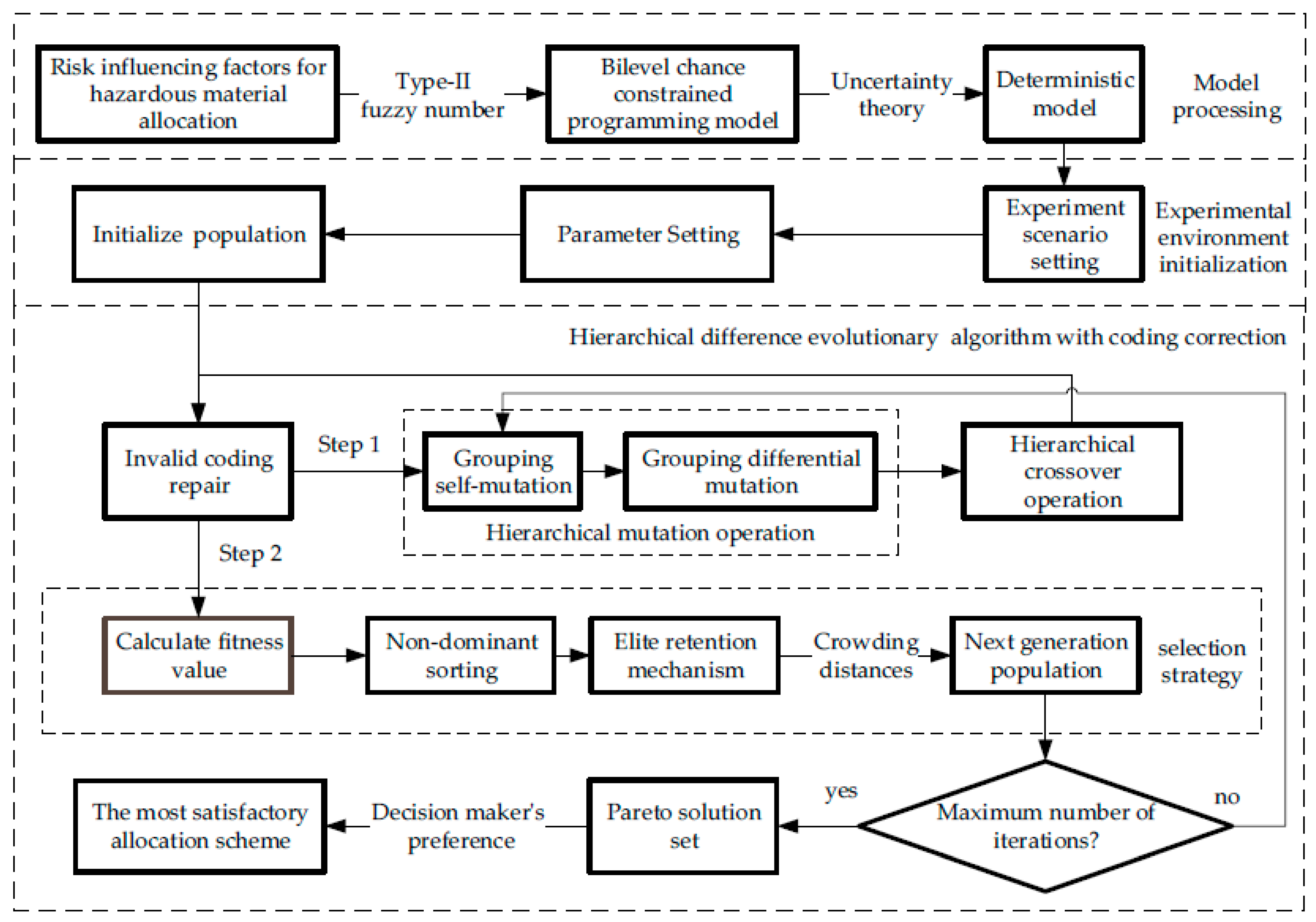
According to the fuzzy chance constrained programming model [30], given confidence levels ${\alpha }^u$ and ${\alpha }^l$, the above type-II fuzzy double-objective optimization model can be transformed into a bilevel chance constrained programming model.

According to the upper level membership function $(r_{ij1}^u,r_{ij2}^u,r_{ij3}^u,r_{ij4}^u,{\omega }_{ij}^u)$ of the allocation risk, the upper level chance constrained programming model can be obtained as follows:

$$\{\begin{array}{l}\min g,\min f^u\\ s.t.\\ Cr\left\{{\displaystyle \sum _{t=1}^T{\displaystyle \sum _{i=1}^N{\displaystyle \sum _{j=1}^N{\tilde{f}}_{tij}}\le f^u}}\right\}\ge {\alpha }^u\\ \mathrm{Equations} (9)\text{–}(12)\end{array}$$

(13)

Similarly, according to the lower level membership function $(r_{ij1}^u,r_{ij2}^u,r_{ij3}^u,r_{ij4}^u,{\omega }_{ij}^u)$, the lower level chance constrained programming model can be obtained as follows:

$$\{\begin{array}{l}\min g,\min f^u\\ s.t.\\ Cr\left\{{\displaystyle \sum _{t=1}^T{\displaystyle \sum _{i=1}^N{\displaystyle \sum _{j=1}^N{\tilde{f}}_{tij}}\le f^u}}\right\}\ge {\alpha }^u\\ \mathrm{Equations} (9)\text{–}(12)\end{array}$$

(14)

Next, according to the confidence equivalent formula of the interval type-II fuzzy model [31], the above opportunity constraints can be converted as follows:

$$\begin{array}{l}Cr\left\{{\displaystyle \sum _{t=1}^T{\displaystyle \sum _{i=1}^N{\displaystyle \sum _{j=1}^N(r_{ij}{}^u\times {\displaystyle \sum _{k=1}^K{x}_{tij}{}^k}})\le f^u}}\right\}\ge {\alpha }^u\Rightarrow {\displaystyle \sum _{t=1}^T{\displaystyle \sum _{i=1}^N{\displaystyle \sum _{j=1}^N(h_{ij}{}^u\times {\displaystyle \sum _{k=1}^K{x}_{tij}{}^k)}}\le f^u}}\\ Cr\left\{{\displaystyle \sum _{t=1}^T{\displaystyle \sum _{i=1}^N{\displaystyle \sum _{j=1}^N(r_{ij}{}^l\times {\displaystyle \sum _{k=1}^K{x}_{tij}{}^k}})\le f^l}}\right\}\ge {\alpha }^l\Rightarrow {\displaystyle \sum _{t=1}^T{\displaystyle \sum _{i=1}^N{\displaystyle \sum _{j=1}^N(h_{ij}{}^l\times {\displaystyle \sum _{k=1}^K{x}_{tij}{}^k}})\le f^l}}\end{array}$$

(15)

where, $Cr\left\{\mathrm{A}\right\}$ represents the degree of confidence of event $\mathrm{A}$, $h_{ij}{}^u$ and $h_{ij}{}^l$ are defined as follows.

$$h_{ij}^u=\{\begin{array}{l}\frac{({\omega }_{ij}^u-2{\alpha }^u)r_{ij1}^u+2{\alpha }^u{r}_{ij2}^u}{{\omega }_{ij}^u},if {\alpha }^u\le \frac{{\omega }_{ij}^u}{2}\\ \frac{2({\omega }_{ij}^u-2{\alpha }^u)r_{ij3}^u+(2{\alpha }^u-{\omega }_{ij}^u)r_{ij4}^u}{{\omega }_{ij}^u},if {\alpha }^u>\frac{{\omega }_{ij}^u}{2}\end{array}$$

(16)

$$h_{ij}^l=\{\begin{array}{l}\frac{({\omega }_{ij}^l-2{\alpha }^l)r_{ij1}^l+2{\alpha }^l{r}_{ij2}^l}{{\omega }_{ij}^l},if {\alpha }^l\le \frac{{\omega }_{ij}^l}{2}\\ \frac{2({\omega }_{ij}^l-2{\alpha }^l)r_{ij3}^l+(2{\alpha }^l-{\omega }_{ij}^l)r_{ij4}^l}{{\omega }_{ij}^l},if {\alpha }^l>\frac{{\omega }_{ij}^l}{2}\end{array}$$

(17)

Combining Equations (13)–(17), the above bilevel chance constrained programming model can be transformed as follows with the weighted method.

$$\{\begin{array}{l}\min g\\ \min f_r=\frac{1}{2}{\displaystyle \sum _{t=1}^T{\displaystyle \sum _{i=1}^N{\displaystyle \sum _{j=1}^N((h_{ij}{}^u+h_{ij}{}^l)\times {\displaystyle \sum _{k=1}^K{x}_{tij}{}^k)}}}}\\ s.t.\\ \mathrm{Equations} (9)\text{–}(12)\end{array}$$

(18)

4. Solution Method

The differential Evolution (DE) algorithm is a global merit-seeking method based on the idea of difference to simulate the survival of the fittest in nature, mainly through mutation, crossover, and selection operations to complete the continuous evolution of the population. Since the hazardous materials allocation studied in this paper only considers the integer batch allocation, which is a kind of large-scale integer programming problem, it is appropriate to use the natural number coding method in the structure of the solution, and the DE algorithm can often find a more excellent solution in solving this kind of problem [32].

The multi-objective differential evolution (MODE) algorithm is the application of the DE algorithm in solving multi-objective optimization problems, and many scholars improved the differential evolution algorithm to different degrees for specific problems [33,34,35]. Considering the multi-dimensional characteristics of the multi-period allocation problem of hazardous materials, which contains multi-periods, multi-reserve points, multi-consumption points, and multi-hazardous material types, in order to improve the search efficiency of the algorithm, the MODE algorithm is improved in this paper by redesigning the crossover operation, variation operation and selection strategy, and designing a coding repair strategy combined with the constraints.

4.1. Structure of Individuals and Initialization of Populations

The above multi-dimensional allocation problem of hazardous materials containing multi-periods, multi-reserve points, multi-consumption points, and multi-hazardous material types can be regarded as a four-dimensional integer programming problem. The structure of the solution can take the form of a three-dimensional integer vector, i.e.,$P=[X_1,\cdots ,X_t,\cdots ,X_T]$, as shown in Figure 3.

Where each matrix $X_t$ represents the hazardous material allocation scheme for each period $t$. Matrix element $x_{tij}=[x_{tij}{}^1,\cdots ,x_{tij}{}^k,\cdots ,x_{tij}{}^K]$ represents the allocation scheme for allocating each type of hazardous material from $a_i$ to $d_j$ in period $t$.

According to the individual structure in Figure 3, the population initialization is completed by coding all individuals in the following way:

$$\begin{array}{l}\forall t=1,2,\dots ,T, \forall i=1,2,\dots ,n, \forall j=1,2,\dots ,m, \forall k=1,2,\dots ,K\\ \mathrm{do}: x_{tij}{}^k\leftarrow \mathrm{randi}[0,\min (c_{tj}{}^k,y_i{}^k)]\\ \hspace{1em}\hspace{1em}\hspace{0.17em}{y}_i{}^k\leftarrow y_i{}^k-x_{tij}{}^k\end{array}$$

where, $\mathrm{randi}[\min ,\max ]$ means to randomly generate an integer between $\min$ and $\max$, and the operation is repeated until the required number $PS$ of individuals for the initial population is satisfied.

4.2. Coding Repair Strategy

During the actual coding operation, there will be problems of individual coding conflicting with constraints, and these coding methods are invalid, which will lead to a large number of infeasible individuals in the evolutionary process of the population, reducing the convergence speed of the population and leading to a decrease in the efficiency of the algorithm search [36]. Therefore, whenever the coding changes, the population coding needs to be checked and repaired to ensure the validity of the individuals of the population and to improve the search efficiency of the solution space. The invalid coding repair strategy is as follows:

Step 1: Calculate the final remaining reserves of each type of hazardous material ${\epsilon }_{Ti}^k\leftarrow y_i^k-{\displaystyle {\sum }_{t=1}^T{x}_{tij}^k}$ at each reserve point after the individual completed all periods of allocation tasks.

Step 2: Check ${\epsilon }_{Ti}^k$. If there exists $i\in \{1,2,\dots ,n\}$ satisfying ${\epsilon }_{Ti}{}^k<0$, it means that the individual has a conflict of reserve quantities at the reserve point. Select the period $t^{\prime }$ when $a_i$ allocates the least quantity in this type $k$ of hazardous materials, and update $x_{t^{\prime }ij}{}^k=0$ and ${\epsilon }_{Ti}^k$. Repeat this step until ${\epsilon }_{Ti}{}^k>0$ for any reserve point $a_i$.

Step 3: Check the allocation risk of each road section in each period. If there exists $t\in \{1,2,\dots ,\mathrm{T}\}$ satisfying $(h_{ij}{}^u+h_{ij}{}^l)\times {\displaystyle {\sum }_{k=1}^K{x}_{tij}{}^k}\ge {\theta }_R$, the allocation risk of this period on this road section is too high to accept. It is necessary to reduce the number of hazardous materials on this road section at this allocation. Randomly select a type of hazardous material $k^{\prime }$ that satisfies $x_{tij}{}^{k^{\prime }}>0$, and do $x_{tij}{}^k\leftarrow x_{tij}{}^k-1$. Repeat this step until $(h_{ij}{}^u+h_{ij}{}^l)\times {\displaystyle {\sum }_{k=1}^K{x}_{tij}{}^k}<{\theta }_R$ exists on any road section.

Step 4: Check the demand satisfaction of each period. $\forall t=1,2,\dots ,T$, if there exist $k\in \{1,\dots ,K\}$ and $j\in \{1,\dots ,m\}$ satisfying ${\displaystyle {\sum }_{i=1}^n{x}_{tij}{}^k<c_{tj}{}^k}$, it means that the demand for hazardous materials of type $k$ at consumption point $d_j$ is not satisfied within that period and additional allocation is required; then, choose randomly a reserve point $a_i$ that satisfies $x_{t{i}^{*}j}{}^k<{\epsilon }_{t{i}^{*}}{}^k$, and complete

$$x_{t{i}^{*}j}{}^k\leftarrow \min \left\{x_{t{i}^{*}j}{}^k+(c_{tj}{}^k-{\displaystyle {\sum }_{i=1}^n{x}_{t{i}^{*}j}{}^k}),{\epsilon }_{t{i}^{*}}{}^k\right\}$$

(19)

Similarly, if there exist $k\in \{1,\dots ,K\}$ and $j\in \{1,\dots ,m\}$ satisfying ${\displaystyle {\sum }_{i=1}^n{x}_{tij}{}^k<c_{tj}{}^k}$, it means that the quantity of hazardous materials allocated in this period is too much, which causes waste of resources; then, randomly select a reserve point $a_{i^{*}}$ meeting $x_{t{i}^{*}j}{}^k>0$, and complete

$$x_{t{i}^{*}j}{}^k\leftarrow \max \left\{x_{t{i}^{*}j}{}^k-({\displaystyle {\sum }_{i=1}^n{x}_{t{i}^{*}j}{}^k-}{c}_t{}^k),0\right\}$$

(20)

After each update of $x_{t{i}^{*}j}{}^k$, update ${\epsilon }_{Ti}^k$ at the same time. Repeat this step until ${\displaystyle {\sum }_{i=1}^n{\displaystyle \sum {}_{j=1}^m{x}_{tij}{}^k=c_t{}^k}}$ is established for demands at all consumption points.

Step 5: Recheck ${\epsilon }_{Ti}^k$ and allocation risks of each road section according to Step 2–4. If all conditions are met, the repair will be completed, otherwise go to the corresponding step of Step 2–4.

4.3. Hierarchical Mutation Operation

In the traditional DE algorithm, coding mutation is mainly carried out by constructing a difference vector. For example, in the DE/rand/1 algorithm [37], three different individuals are randomly selected from the initial population, and the mutation operation is performed by constructing a difference vector by the following equation to obtain new individuals:

$$X_t^{p^{*}}\leftarrow X_t^{p^1}+F\times (X_t^{p^2}-X_t^{p^3})$$

(21)

where $F$ is the scaling factor, and $F=1$ considering the value limitation of individual coding. To ensure that the quantity of hazardous materials allocated will not be negative, take the absolute value of the above difference vector.

$$X_t^{p^{*}}\leftarrow X_t^{p^1}+F\times |X_t^{p^2}-X_t^{p^3}|$$

(22)

For the multi-period allocation scheme problem of hazardous materials proposed in this paper, considering the different selection schemes of reserve points and consumption points at different periods among individuals, the allocation schemes between reserve points and consumption points of new individuals obtained from the difference vector constructed by Equation (22) tend to be more dispersed, which makes the number of reserve points involved in allocation at each period greatly increased in new individuals, and although it enriches the diversity of individuals in the population, the new individuals produced are often of low quality, which is not conducive to the evolution of the population. Therefore, in order to improve the quality of the population, we consider grouping differential mutation based on the selection sequence of the same reserve points in each period of the allocation scheme to optimize the evolutionary direction of the population.

In order to solve the problem of population diversity decline and easily fall into the local optimum brought by population grouping differential mutation. Combined with the three-dimensional integer vector coding structure of individual in Figure 3, and referring to the two-point mutation strategy in genetic algorithm [38], each individual coding in the initial population is firstly subjected to a hierarchical progressive self-mutation operation in three dimensions from period scheme layer $(X_1,\dots ,X_T)$, reserve point scheme layer $(x_{t1},\dots ,x_{tn})$, and consumption point scheme layer $(x_{ti1}^{},\dots ,x_{tim}^{})$ according to certain probability.

$$\begin{array}{l}\mathrm{if} c>r_1\\ \forall x_{ti},(\dots ,x_{ti{a}_2}^{},\dots ,x_{ti{a}_1}^{},\dots )\leftarrow (\dots ,x_{ti{a}_1}^{},\dots ,x_{ti{a}_2}^{},\dots ) \\ \hspace{1em}\hspace{1em}\mathrm{if} c>r_2\\ \hspace{1em}\hspace{1em}\hspace{1em}\forall X_t,(\dots ,x_{ta2},\dots ,x_{ta1},\dots )\leftarrow (\dots ,x_{ta1},\dots ,x_{ta2},\dots )\\ \hspace{1em}\hspace{1em}\hspace{1em}\mathrm{if} c>r_3\\ \hspace{1em}\hspace{1em}\hspace{1em}\hspace{1em}(\dots ,X_{a2},\dots ,X_{a1},\dots )\leftarrow (\dots ,X_{a1},\dots ,X_{a2},\dots )\\ \hspace{1em}\hspace{1em}\hspace{1em}\mathrm{end} \mathrm{if}\\ \hspace{1em}\hspace{1em}\mathrm{end} \mathrm{if}\\ \mathrm{end} \mathrm{if} \end{array}$$

where,$c=\mathrm{rand}[0,1]$, $r_1$, $r_2$ and $r_3$ are the probabilities of mutation at different levels, respectively.

The initial population $P_0$ is grouped according to the same reserve point selection sequence, and after expanding the number of individuals in the group by performing two self-mutation operations on each group element separately, individuals are selected from the same group element to construct new individuals according to Equation (22), and the operation is repeated until a new population $P_1$ is generated.

4.4. Hierarchical Crossover Operation

In order to enrich the diversity of population individuals and improve the search efficiency of the Pareto solution set, similarly, crossover operations can be completed for individuals from three levels: period scheme layer, reserve point scheme layer, and consumption point scheme layer according to the structure of individual in Figure 3.

Individuals $p_0$ and corresponding $p_1$ are randomly selected from the initial population $P_0$ and its hierarchical mutation population $P_1$. After the crossover probabilities are determined, and the crossover operation can be completed by assigning one from the period scheme layer, reserve the point scheme layer and consumption point scheme layer to produce two new individuals $p_2$ and $p_3$ according to the random interval probabilities, as shown in Figure 4.

Continue to select the remaining individuals in the population, and repeat the hierarchical crossover operation in Figure 4 until two new populations $P_2$ and $P_3$ are generated.

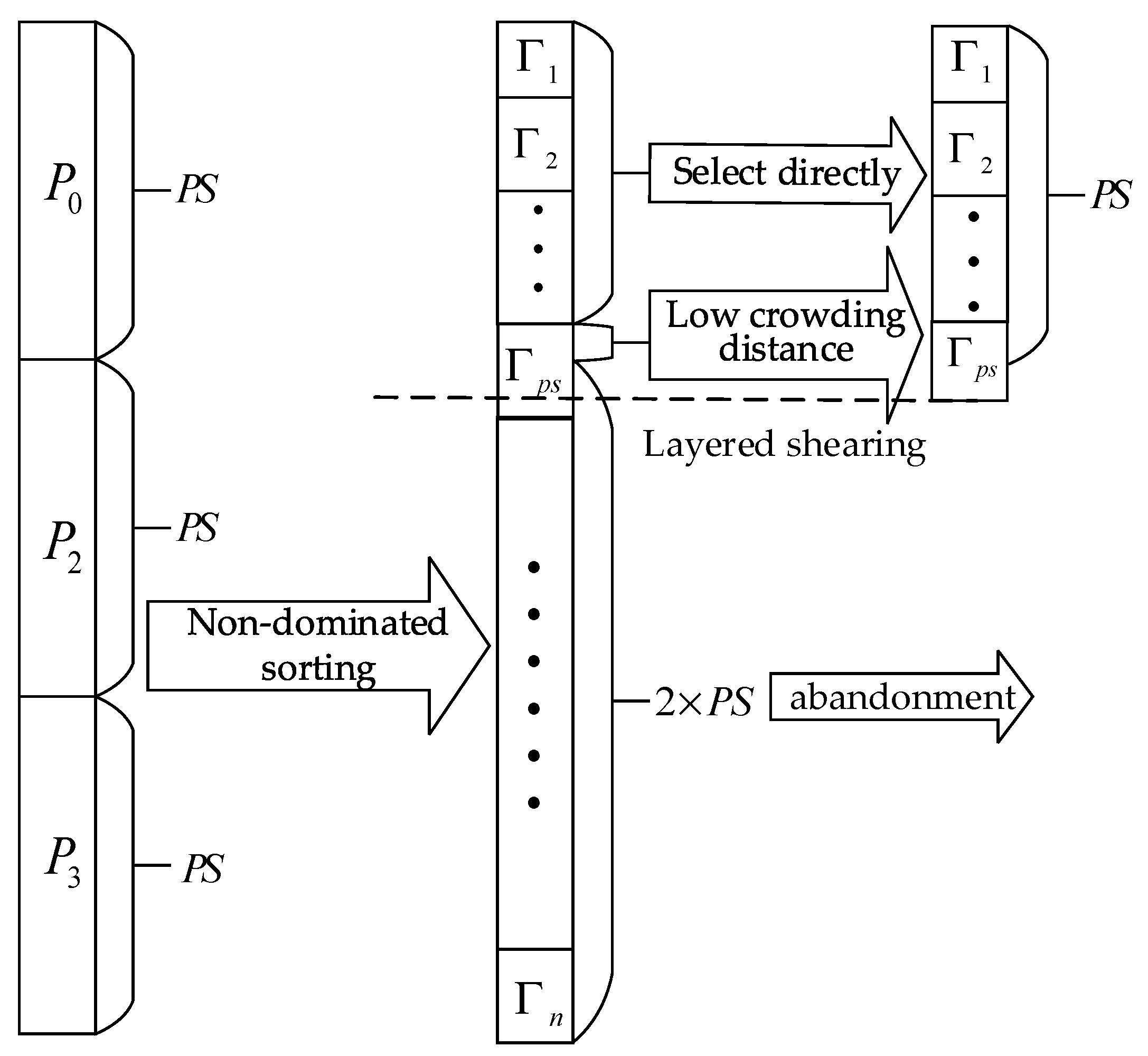
4.5. Population Selection Strategy

Calculate the fitness values of all individuals in the initial population and two crossover populations $P_2$ and $P_3$, that is, the cumulative number of reserve points participating in the allocation and the cumulative allocation risk. The concepts of Pareto non-dominated sorting and individual crowding distance in non-determined sorting genetic algorithm (NSGA) are introduced to cut the population hierarchically [39], and the $PS$ optimal individuals are retained as the initial population $P_0^1$ of the next iteration according to the elite retention mechanism. The steps are as follows:

Step 1: Calculate the double-objective fitness value of all individuals, determine the dominance relationship between each individual according to the non-dominance ranking, and retain the non-dominated individuals in it as the first Pareto frontier ${\mathsf{\Gamma }}_1$.

Step 2: Individuals in ${\mathsf{\Gamma }}_1$ are removed from the three populations above, the dominance relationships among the remaining individuals are determined again, and the non-dominant individuals among them are retained as the second Pareto frontier ${\mathsf{\Gamma }}_2$. The process is repeated until the hierarchy of all individuals is divided.

Step 3: The optimal individuals are retained as the initial population for the next iteration according to the hierarchical relationship. The more advanced the hierarchy, the better the quality of the individual solution. If the number of individuals exceeds $PS$ in the hierarchical retention, the last layer to be retained is cut according to the individual crowding distance, and the individuals with smaller crowding distance are removed to meet the population size $PS$. The population selection strategy is shown in Figure 5.

Crowding distance is generally used to describe the size of the density around individuals and the retention of individuals with larger crowding distance makes the preserved individuals less similar and maintains the diversity of the population. The crowding distance is calculated by the following equation.

$${\sigma }_x=\frac{g_{x+1}-g_{x-1}}{g_{\max }-g_{\min }}+\frac{f_{x+1}-f_{x-1}}{f_{\max }-f_{\min }}$$

(23)

where $g_{x+1}$, $g_{x-1}$, $f_{x+1}$ and $f_{x-1}$ are the corresponding values taken by the individuals before and after in the Pareto frontier of the individual when sorted by the number of cumulative reserve points participating in the allocation and cumulative allocation risk, respectively; $g_{\max }$, $g_{\min }$, $f_{\max }$ and $f_{\min }$ are the maximum and minimum values of the number of cumulative reserve points participating in the allocation and cumulative allocation risk on the Pareto frontier of the individual, respectively.

5. Examples and Results

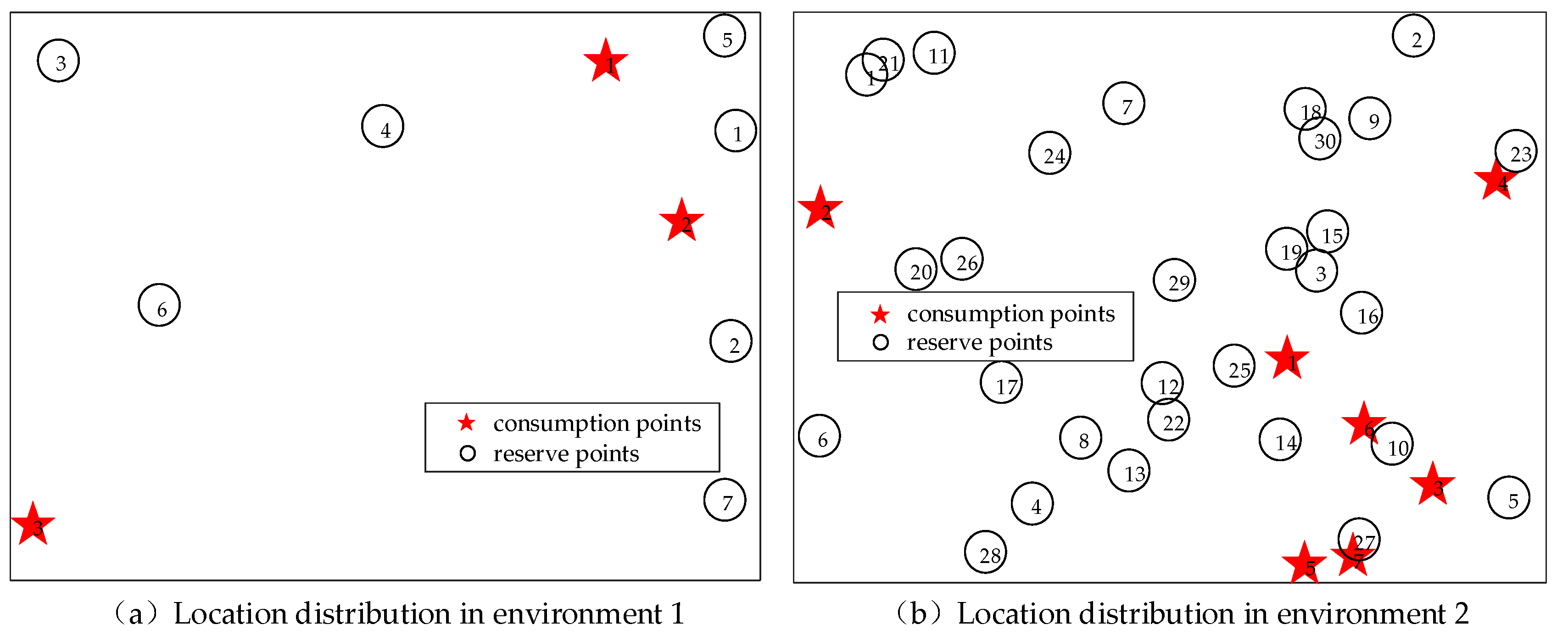
5.1. Experimental Scene Setup

The HDA-CR proposed in Section 3 is an improvement on the coding repair and non-determined sorting-based differential evolution (ERNS-DE) algorithm proposed in literature [40], which aims to solve the problem of multi-dimensional allocation problem of hazardous materials. The parameters of HDA-CR are set as shown in

Table 2. The parameter setting of HDA-CR.

Population Size	Self-Mutation Probability	Scaling Factor	Hierarchical Coefficient	Crossover Probability	Maximum Number of Iterations
30	(0.1 0.5 0.8)	1	(0.3 0.6)	0.5	500

.

Considering the lack of relevant hazardous materials transfer risk data, in order to verify the effectiveness of the model and algorithm as much as possible, this example contains two different scale experimental environment settings, two hazardous materials supply and demand scenarios, and two periods settings, including long-term allocation and short-term allocation, as well as a total of eight difference experimental scenarios, comparing HDA-CR with the classical multi-objective algorithm and the ERNS-DE algorithm in different scenarios.

Environment 1: Consider the smaller area hazardous material allocation problem, four hazardous material types, seven reserve points, and three consuming points, and the locations of the reserve points and consuming points are randomly generated according to the generalized distance, as shown in Figure 6a. The numbers in Figure 6 represent the numbering of consumption points and reserve points respectively.

Environment 2: Consider the larger area hazardous material allocation problem, 7 hazardous material types, 30 reserve points, and 7 consumption points, and the locations of reserve and consumption points are randomly generated according to the generalized distance, as shown in Figure 6b.

Case 1: Consider hazardous materials allocation problem under resource-rich. The sum of the quantities of hazardous materials available at all reserve points is far greater than the sum of the demands at all consumption points in all periods.

$${\displaystyle \sum _{i=1}^T{y}_i{}^k\gg {\displaystyle \sum _{t=1}^T{c}_t{}^k,k=1,2,\dots K}}$$

(24)

Case 2: Consider the hazardous materials allocation problem under resource constraints. The sum of the quantities of hazardous materials available at all reserve points is exactly equal to the sum of the demands of all consumption points in all periods.

$${\displaystyle \sum _{i=1}^T{y}_i{}^k={\displaystyle \sum _{t=1}^T{c}_t{}^k,k=1,2,\dots K}}$$

(25)

Period parameter setting: Consider the short-term allocation problem of hazardous materials, and let the number of periods $T=5$; consider the long-term allocation problem of hazardous materials, and let the number of periods $T=24$. The specific experimental scenarios are set up as shown in

Table 3. Experimental scenarios settings.

Experimental Scenarios	Environment Settings	Supply and Demand Cases	Period Numbers
Sce 1	Environment 1	Case 1	5
Sce 2	Environment 1	Case 2	5
Sce 3	Environment 2	Case 1	5
Sce 4	Environment 2	Case 2	5
Sce 5	Environment 1	Case 1	24
Sce 6	Environment 1	Case 2	24
Sce 7	Environment 2	Case 1	24
Sce 8	Environment 2	Case 2	24

.

In this experiment, the traffic accident probabilities $p{j}_{ij}^l$ and $p{j}_{ij}^u$, population density $p{d}_{ij}^l$ and $p{d}_{ij}^u$, the influence range $s^l$ and $s^u$ of hazardous materials, and the membership values ${\omega }_{ij}^l$ and ${\omega }_{ij}^u$ of upper and lower layers on each road section are randomly selected from the interval $[0.001 0.009]$, $[0.01 0.02]$, $[90 110]$, $[140 160]$, $[200 500]$, $[1500 2000]$, $[0 0.5]$, and $[0.5 1]$, respectively. Additionally, ${\theta }_R=100$ is adopted as the allocation risk threshold.

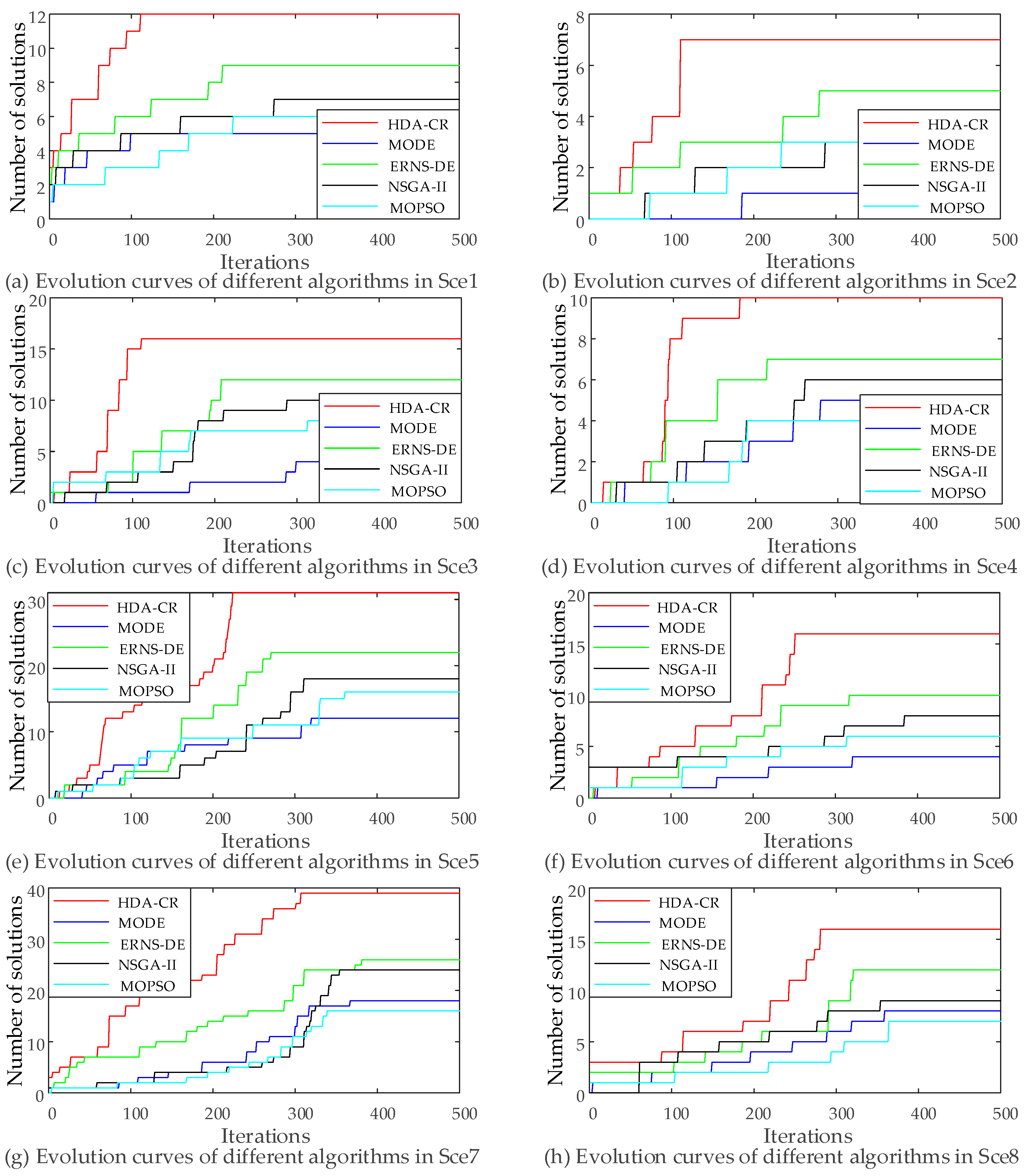
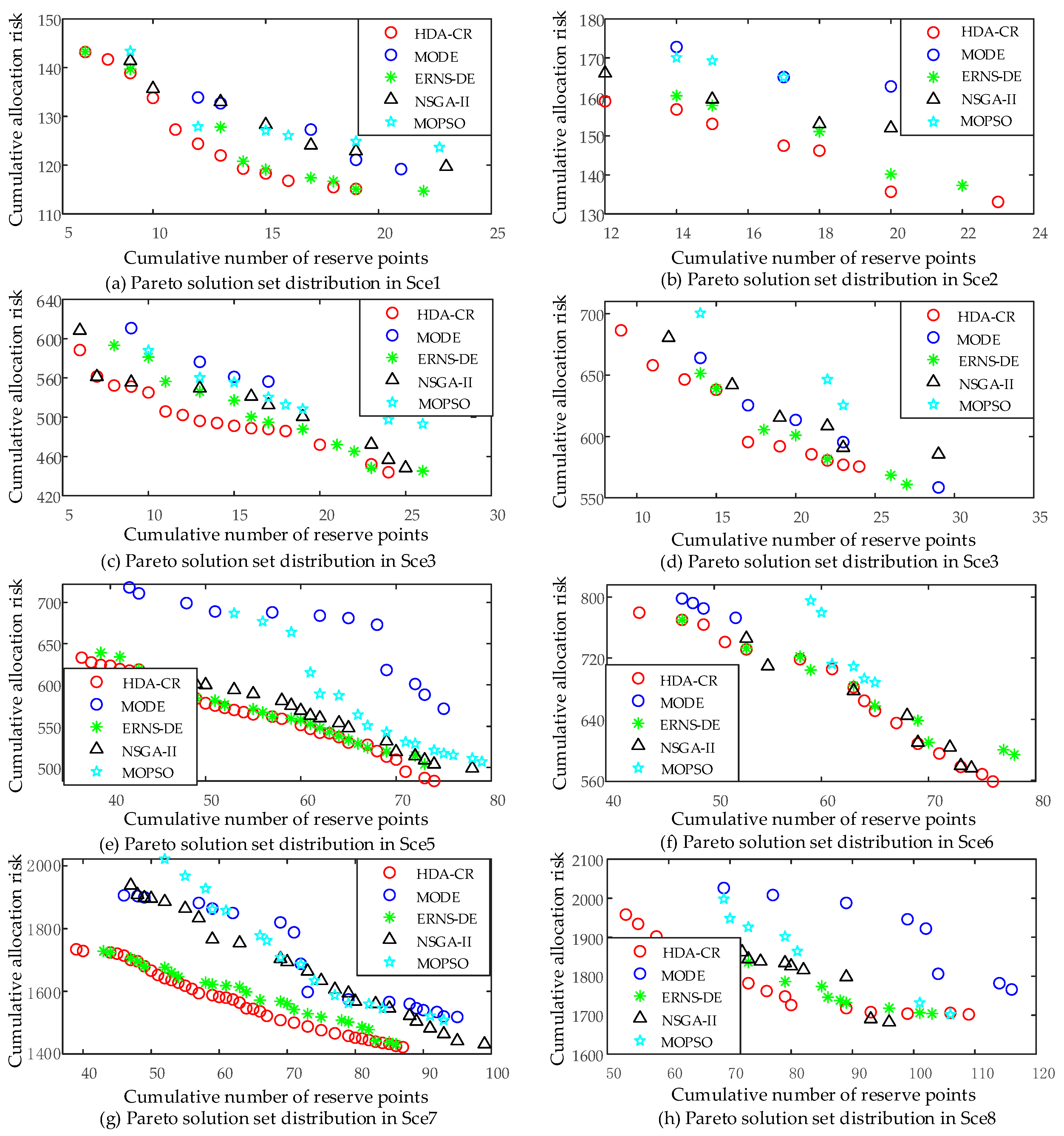
5.2. Algorithm Comparison Analysis

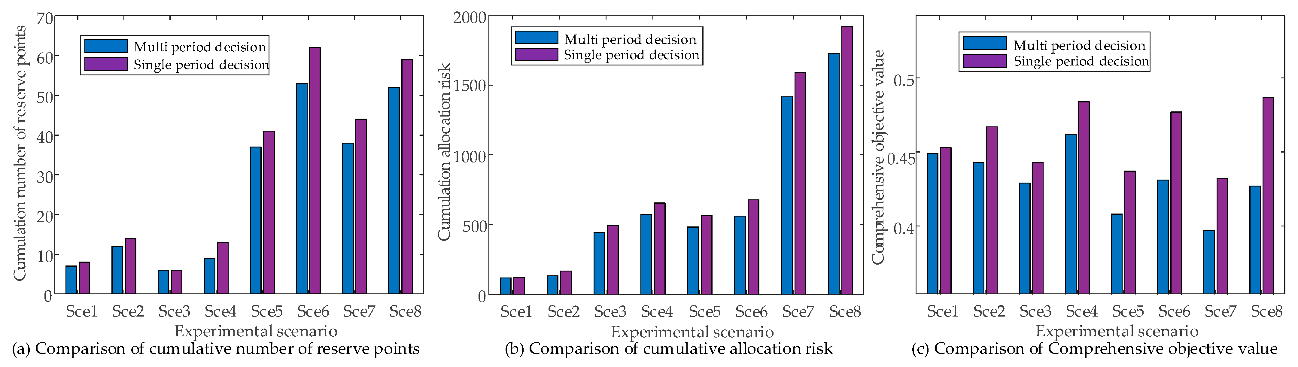
In order to test the performance of HDA-CR proposed in this paper and solve the multi-period allocation model of hazardous materials, HDA-CR is compared with the traditional MODE, the single period multi-dimensional allocation problem solving algorithm (ERNS-DE) in literature [40], as well as other classical multi-objective algorithms, such as NSGA-II [41] and multi-objective particle swarm optimization (MOPSO) [42], by combining the double-objective optimization model in Equation (18) and setting the confidence level ${\alpha }^u={\alpha }^l=0.05$. Among them, the basic parameters of MODE and ERNS-DE are consistent with the corresponding parameter settings in Table 2. NSGA-II and MOPSO use the corresponding parameters in literature [41] and literature [42], respectively.

Figure 7a–h shows the comparison of the Pareto optimal solution evolution curves of five algorithms for solving the multi-objective model of the multi-period allocation of hazardous materials (Equation (18)) under different scenarios. It can be seen from the evolution curves of the Pareto optimal solution under eight scenarios that HDA-CR converges faster than other algorithms, and the size of Pareto solution space searched is larger than other algorithms. For example, as shown in Figure 7a, the evolution curve of the HDA-CR converges after about 120 iterations and can search 12 Pareto optimal solutions in Scenario 1, while other algorithms converge relatively slowly and the number of Pareto optimal solutions searched does not exceed 9. It shows that HDA-CR can effectively improve the diversity of the population in the experimental scenario and accelerate the evolution efficiency of the population compared with other algorithms. In addition, it can be seen from the comparison results of (a–d) and (e–h) in Figure 7 that with the increase in the number of periods, the above five algorithms need more iterations to converge, but the advantages of HAD-CR still exist, and a greater difference in the number of Pareto optimal solutions is found. This indicates that HDA-CR has a better solution effect in the long-term allocation of hazardous materials. For example, Figure 7a,e is in the same experimental environment and resource configuration. In Figure 7e, HDA-CR can search 30 Pareto optimal solutions, and other algorithms can search no more than 23 Pareto optimal solutions. This shows that HDA-CR has more obvious search advantages when considering the number of allocated periods is 24 rather than 5.

Figure 8 shows the distribution of the Pareto solution set obtained by the above five algorithms in different scenarios clearly. According to the properties of the Pareto solution, it can be seen intuitively that the Pareto optimal solution obtained by HDA-CR is superior to the other four algorithms in terms of quantity and scale in different scenarios. For example, Figure 8h shows the distribution of two objective function values of the Pareto solution obtained by five algorithms in the multi-period allocation model of hazardous materials (Equation (18)) under Scenario 8. It can be seen that the distribution of Pareto solution set searched by HDA-CR is more uniform and the quality is obviously superior (the smaller the values of the two objective functions, the higher the quality of the solution).

In order to compare the quantity of Pareto optimal solutions of different algorithms more accurately, the average running time (T), two-set coverage (SC), and hypervolume (HV) of the algorithms are selected to further compare the optimization performance of each algorithm from the perspectives including computational cost, accuracy, diversity, and convergence of Pareto optimal solution, respectively.

1. Average running time (T): it indicates the average time of algorithm running, which can be used to measure the time complexity of each algorithm, and the smaller the value, the higher the computational efficiency of the algorithm.

$$\mathrm{T}=\frac{1}{N}{\displaystyle \sum _{i=1}^N{\mathrm{T}}_{\mathrm{i}}}$$

(26)

where ${\mathrm{T}}_i$ is the time consumption of each independent operation and $N$ is the number of independent runs of the algorithm.

2. Two-set coverage (SC) [43]: also known as $C$ metric, it is used to compare the accuracy of the Pareto solutions obtained by each algorithm, and its lower value indicates the better quality of the Pareto solution set.

$$C(\mathrm{A},B)=\frac{1}{N}{\displaystyle \sum _{i=1}^N\frac{\left|b\in {\mathrm{B}}_i|\exists a\in {\mathrm{A}}_i:a\prec b\right|}{\left|{\mathrm{B}}_i\right|}}$$

(27)

where the set ${\mathrm{A}}_i$ and the set ${\mathrm{B}}_i$ are the sets of Pareto solutions obtained by different algorithms in each operation, respectively, and $a\prec b$ indicates that the individual $a$ is dominated by the individual $b$. For comparison, the ERNS-DE is chosen as the benchmark algorithm to compare the accuracy of Pareto solutions obtained by the HDA-CR with the other three algorithms in this paper; when calculating the two-set coverage of ERNS-DE, the HDA-CR is chosen as the benchmark algorithm to calculate and compare the two-set coverage with that of HDA-CR in a two-by-two comparison.

3. Hypervolume (HV) [44]: It is used to measure the ratio of the size width of the Pareto solution set obtained by the algorithm in the area covered by the target space, and this index can measure the convergence and diversity of the algorithm at the same time. The larger the value, the more uniform the individual distribution and better the convergence of the Pareto solution set obtained by the algorithm.

$$\mathrm{HV}=\frac{1}{N}{\displaystyle \sum _{i=1}^N\mathrm{volume}({\displaystyle \underset{i=1}{\overset{\left|{\mathrm{A}}_i\right|}{\cup }}{v}_i})}$$

(28)

where $v_i$ is the hypervolume enclosed between the reference point and individual $i$. After normalizing the fitness values of the individuals, the point (1,1) is selected as the reference point.

According to the above multi-objective algorithm evaluation index, the values of each index of different algorithms under different scenarios are calculated, and the results are shown in

Table 4. Evaluation results of the algorithm performance indicators.

Experimental Scenarios	HDA-CR			MODE			ERNS-DE			NSGA-II			MOPSO
	T	SC	HV	T	CS	HV	T	CS	HV	T	CS	HV	T	CS	HV
Sce 1	6.918	0.111	0.625	6.508	0.6	0.122	6.376	0.583	0.462	7.216	0.6	0.371	7.700	0.6	0.128
Sce 2	5.756	0	0.688	4.929	0.444	0.387	4.308	0.714	0.584	3.355	0.667	0.428	5.710	0.556	0.411
Sce 3	10.429	0.083	0.642	11.281	0.429	0.483	9.711	0.562	0.573	12.327	0.714	0.477	13.192	0.571	0.209
Sce 4	9.301	0	0.655	5.721	0.5	0.241	8.220	0.5	0.523	6.951	0.5	0.507	10.518	0.667	0.350
Sce 5	18.964	0.091	0.462	19.291	0.4	0.084	18.192	0.612	0.407	21.300	0.1	0.410	22.221	0.6	0.217
Sce 6	17.397	0.1	0.687	11.278	0.546	0.197	16.406	0.5	0.635	13.690	0.636	0.523	19.2914	0.723	0.342
Sce 7	22.140	0	0.753	21.812	0.667	0.172	21.464	0.564	0.658	22.308	0.5	0.560	22.904	0.5	0.418
Sce 8	21.402	0.083	0.799	17.315	0.692	0.452	20.174	0.562	0.725	19.157	0.885	0.504	18.207	0.615	0.431

.

As can be seen from the comparison of the three indicators in Table 4, the HDA-CR proposed in this paper can effectively improve the quality of the solutions in the Pareto optimal solution set searched for at the expense of certain time resources, and outperforms other algorithms in terms of solution accuracy, diversity, and convergence; at the same time, it can effectively alleviate the resource conflict problem, reducing the cost of computing in resource-constrained scenarios. As for the formulation of multi-period allocation schemes for hazardous materials, the main purpose is to determine the optimal long-term allocation scheme, that is, to ensure the quality of the Pareto solution, so that the hazardous materials at each reserve point are consumed in an orderly and reasonable manner, and the running time of the algorithm can be disregarded. Therefore, it can be considered that the HDA-CR performs better in the multi-period resource allocation of hazardous materials.

5.3. Discussion

The solution obtained by the above method is often a set of Pareto solution sets, that is, a set of generally incomparable compromise solutions, while the decision process usually needs to provide the decision-maker with the optimal solution choice. The decision-maker’s preference weight $w$ can be introduced to select the optimal solution satisfying the decision-maker from the Pareto solution set.

$$\min w{g}^{\prime }+(1-w)f_r^{\prime }$$

(29)

where $g^{\prime }$ and $f_r^{\prime }$ are the normalized objective function values, and different preference weights are selected according to the decision-maker’s preference for different objectives to provide the decision-maker with the corresponding most appropriate multi-period allocation scheme of hazardous materials. Figure 9 shows the allocation scheme with the lowest number of reserve points participating in allocation in Sce 1.

From the perspective of material allocation, the current research mainly focuses on the allocation of hazardous materials in a single period, where the best scheme for the allocation of hazardous materials is found from different perspectives and methods. For example, in literature [10], transportation risk, transportation time, and fuel consumption are considered to find the optimal distribution network. However, from the perspective of supply and demand, the supply and demand relationship will change dynamically in each period. It is not enough to consider only the optimal scheme setting in a single period.

In order to further compare the impact of single-period and multi-period decision making methods on hazardous material allocation scheme. The proposed method in this paper is compared with the traditional single-period decision making method under different scenarios to calculate the cumulative number of reserve point participating allocation tasks, the cumulative allocation risk, and the comprehensive objective value. The results are shown in Figure 10 and the comprehensive objective value is defined as follows:

$$E=\hspace{1em}\frac{f-f_{\min }}{2(f_{\max }-f_{\min })}+\frac{g-g_{\max }}{2(g_{\max }-g_{\min })}$$

(30)

where $f_{\max }$, $f_{\min }$, $g_{\max }$ and $g_{\min }$ are the maximum and minimum values of the cumulative allocation risk and cumulative number of reserve points participating in the allocation, respectively, in the Pareto solution under the difference scenarios.

The traditional decision making approach only considers the optimal target of this period when developing the allocation scheme without considering the future allocation of hazardous materials. From the comparison results in Figure 10, it can be seen clearly that the integrated consideration of multiple periods can lead to a safer and more suitable ideal allocation scheme. Moreover, in the scenario of long-term allocation and limited resources, the comparison of the two decision methods becomes more and more obvious. For example, as shown in Figure 10a, the cumulative numbers of reserve points of the two decision making methods are both 6 in Scenario 3; there is no difference between them and the difference is also small in Scenario 1. However, when resources are limited or the number of periods increases, the multi-period decision making method can obtain an allocation scheme with fewer cumulative reserve points participating in allocation, and the difference between them is larger, which can be seen from the comparison results of Scenario 2, Scenario 4, Scenario 5, Scenario 6, Scenario 7, and Scenario 8 in Figure 10a. Therefore, it is very important for the sustainable management of hazardous materials to develop a suitable multi-period allocation scheme of hazardous materials.

6. Conclusions

This paper solves the problem of formulating the optimal allocation scheme of hazardous materials and realizing the sustainable management of hazardous materials. Firstly, it abstractly models the realistic situation that needs to be considered for the multi-period allocation scheme of hazardous materials under uncertainty, and gives a Bilevel chance constrained programming model for formulating a double-objective multi-period allocation scheme of hazardous materials that considers the minimum cumulative number of reserve points participating in the allocation and the minimum cumulative allocation risk. Then, we improved the differential evolution algorithm and established a hierarchical difference evolution algorithm considering multi-dimensional problems to solve the model and find the optimal allocation scheme of hazardous materials.

The experience results provide the following conclusions: (1) In solving the multi-period allocation model, the hierarchical differential evolution algorithm converges faster than the other multi-objective evolution algorithm, and can search more Pareto solutions, which means there is more space for selecting the optimal allocation scheme. (2) The Pareto solution set obtained by the hierarchical difference algorithm is densely and evenly distributed between the cumulative allocation risk and the cumulative number of reserve points participating in the allocation, with high similarity, and better solution quality (the quality of the searched allocation scheme set is better). (3) Compared with the single-period decision making method, the method proposed in this paper can obtain a safer and more efficient hazardous material allocation scheme, which is conducive to the sustainable management of hazardous materials.

The practical implications of this study include the following: (1) Type-II fuzzy numbers are used in the hazardous materials allocation model proposed in Section 3.3 to measure the transportation risk in the hazardous materials allocation process, which provides a new measurement method for the subsequent risk assessment of nuclear materials, explosives, hazardous chemicals, and other hazardous materials. (2) This study can solve the long-term allocation scheme of hazardous materials from a global perspective, and realizes that multiple storage points can allocate multiple hazardous material resources for multiple distribution points in a coordinated manner without causing resource conflicts, which provides a certain method reference for the subsequent solution to the long-term optimal allocation of large-scale resources in industrial production. (3) This paper designs a new hierarchical differential evolution algorithm, which provides an alternative global optimization algorithm for subsequent solution of multi-dimensional and multi-objective task allocation problems.

It is worth noting that the method is proposed to make a multi-period scheduling plan for hazardous materials on the basis of inherent inventory without considering the replenishment of inventory, the uncertainty of demand at each consumption point in each period, and the inherent attributes of each hazardous material, such as residual life, economic benefits, and other factors, which cannot be ignored when making a long-term allocation scheme for hazardous materials, and further research is still needed in the follow-up work.

References

1. Gawlik-Kobylińska, M. Current Issues in Combating Chemical, Biological, Radiological, and Nuclear Threats to Empower Sustainability: A Systematic Review. Appl. Sci. 2022, 12, 8315. [Google Scholar] [CrossRef]
2. Izdebski, M.; Jacyna-Goda, I.; Goda, P. Minimisation of the probability of serious road accidents in the transport of hazardous materials. Reliab. Eng. Syst. Saf. 2022, 217, 108093. [Google Scholar] [CrossRef]
3. Zografos, K.G.; Androutsopoulos, K.N. A heuristic algorithm for solving hazardous materials distribution problems. Eur. J. Oper. Res. 2004, 152, 507–519. [Google Scholar] [CrossRef]
4. Li, S.; Zu, Y.; Fang, H.; Liu, L.; Fan, T. Design Optimization of a HAZMAT Multimodal Hub-and-Spoke Network with Detour. Int. J. Environ. Res. Public Health 2021, 18, 12470. [Google Scholar] [CrossRef]
5. Saat, M.R.; Barkan, C.P.L. Generalized railway tank car safety design optimization for hazardous materials transport: Addressing the trade-off between transportation efficiency and safety. J. Hazard. Mater. 2011, 189, 62–68. [Google Scholar] [CrossRef] [PubMed]
6. Liu, L.; Wu, Q.; Li, S.; Li, Y.; Fan, T. Risk Assessment of Hazmat Road Transportation Considering Environmental Risk under Time-Varying Conditions. Int. J. Environ. Res. Public Health 2021, 18, 9780. [Google Scholar] [CrossRef]
7. Korytárová, J.; Hromádka, V. Risk Assessment of Large-Scale Infrastructure Projects—Assumptions and Context. Appl. Sci. 2021, 11, 109. [Google Scholar] [CrossRef]
8. Park, B.-C.; Lim, C.; Oh, S.-J.; Lee, J.-E.; Jung, M.-J.; Shin, S.-C. Development of Fire Consequence Prediction Model in Fuel Gas Supply System Room with Changes in Operating Conditions during Liquefied Natural Gas Bunkering. Appl. Sci. 2022, 12, 7996. [Google Scholar] [CrossRef]
9. Krejci, L. Risk analysis of hazardous materials transportation. Int. Verk. 2019, 71, 43–45. [Google Scholar]
10. Verter, V.; Kara, B.Y. A GIS-based framework for hazardous materials transport risk assessment. Risk Anal. 2001, 21, 1109–1120. [Google Scholar] [CrossRef] [PubMed] [Green Version]
11. Topuz, E.; Talinli, I.; Aydin, E. Integration of environmental and human health risk assessment for industries using hazardous materials: A quantitative multi criteria approach for environmental decision makers. Environ. Int. 2011, 37, 393–403. [Google Scholar] [CrossRef] [PubMed]
12. Zhang, W.; Huang, Z.; Zhang, J.; Zhang, R.; Ma, S. Multifactor Uncertainty Analysis of Construction Risk for Deep Foundation Pits. Appl. Sci. 2022, 12, 8122. [Google Scholar] [CrossRef]
13. Holeczek, N. Hazardous materials truck transportation problems: A classification and state of the art literature review. Transp. Res. Part D Transp. Environ. 2019, 69, 305–328. [Google Scholar] [CrossRef]
14. Kazantzi, V.; Kazantzis, N.; Gerogiannis, V.C. Risk informed optimization of a hazardous material multi-periodic transportation model. J. Loss Prev. Process Ind. 2011, 24, 767–773. [Google Scholar] [CrossRef]
15. Du, J.; Li, X.; Yu, L.; Dan, R.; Zhou, J. Multi-depot vehicle routing problem for hazardous materials transportation: A fuzzy bilevel programming. Inf. Sci. 2017, 399, 201–218. [Google Scholar] [CrossRef]
16. Zero, L.; Bersani, C.; Sacile, R.; Laarabi, M.H. Bi-objective shortest path problem with one fuzzy cost function applied to hazardous materials transportation on a road network. In Proceedings of the 2016 11th System of Systems Engineering Conference (SoSE), Kongsberg, Norway, 12–16 June 2016; pp. 1–5. [Google Scholar]
17. Yan, S.; Wang, S.S.; Chang, Y.H. Cash transportation vehicle routing and scheduling under stochastic travel times. Eng. Optim. 2014, 46, 289–307. [Google Scholar] [CrossRef]
18. Pamučar, D.; Ljubojević, S.; Kostadinović, D.; Đorović, B. Cost and risk aggregation in multi-objective route planning for hazardous materials transportation-A neuro-fuzzy and artificial bee colony approach. Expert Syst. Appl. 2016, 65, 1–15. [Google Scholar] [CrossRef]
19. Berglund, P.G.; Kwon, C. Robust facility location problem for hazardous waste transportation. Netw. Spat. Econ. 2014, 14, 91–116. [Google Scholar] [CrossRef]
20. Zhou, Y.; He, J.; Nie, Q. A comparative runtime analysis of heuristic algorithms for satisfiability problems. Artif. Intell. 2009, 173, 240–257. [Google Scholar] [CrossRef] [PubMed] [Green Version]
21. Berliński, M.; Warchulski, E.; Kozdrowski, S. Applications of Metaheuristics Inspired by Nature in a Specific Optimisation Problem of a Postal Distribution Sector. Appl. Sci. 2022, 12, 9384. [Google Scholar] [CrossRef]
22. Rathore, N.; Jain, P.K.; Parida, M. A Sustainable Model for Emergency Medical Services in Developing Countries: A Novel Approach Using Partial Outsourcing and Machine Learning. Risk Manag. Healthc. Policy 2022, 15, 193–218. [Google Scholar] [CrossRef] [PubMed]
23. Ma, C.; Hao, W.; Pan, F.; Xiang, W. Road screening and distribution route multi-objective robust optimization for hazardous materials based on neural network and genetic algorithm. PLoS ONE 2018, 13, e0198931. [Google Scholar] [CrossRef]
24. Bula, G.A.; Prodhon, C.; Gonzalez, F.A.; Afsar, H.M.; Velasco, N. Variable neighborhood search to solve the vehicle routing problem for hazardous materials transportation. J. Hazard. Mater. 2017, 324 Pt B, 472–480. [Google Scholar] [CrossRef]
25. Zero, L.; Bersani, C.; Paolucci, M.; Sacile, R. Two new approaches for the bi-objective shortest path with a fuzzy objective applied to HAZMAT transportation. J. Hazard. Mater. 2019, 375, 96–106. [Google Scholar] [CrossRef]
26. Kaup, M.; Łozowicka, D.; Baszak, K.; Ślączka, W.; Kalbarczyk-Jedynak, A. Risk Analysis of Seaport Construction Project Execution. Appl. Sci. 2022, 12, 8381. [Google Scholar] [CrossRef]
27. Erkut, E.; Verter, V. Modeling of Transport Risk for Hazardous Materials. Oper. Res. 1998, 46, 625–642. [Google Scholar] [CrossRef] [Green Version]
28. Ohn, S.W.; Namgung, H. Interval Type-II Fuzzy Inference System Based on Closest Point of Approach for Collision Avoidance between Ships. Appl. Sci. 2020, 10, 3919. [Google Scholar] [CrossRef]
29. Pramanik, S.; Jana, D.K.; Mondal, S.K.; Maiti, M. A fixed-charge transportation problem in two-stage supply chain network in Gaussian type-II fuzzy environments. Inf. Sci. 2015, 325, 190–214. [Google Scholar] [CrossRef]
30. Liu, Z.Q.; Liu, Y.K. Type-II fuzzy variables and their arithmetic. Soft Comput. 2010, 14, 729–747. [Google Scholar] [CrossRef]
31. Kundu, P.; Majumder, S.; Kar, S.; Maiti, M. A method to solve linear programming problem with interval type-II fuzzy parameters. Fuzzy Optim. Decis. Mak. 2019, 18, 103–130. [Google Scholar] [CrossRef]
32. Eltaeib, T.; Mahmood, A. Differential Evolution: A Survey and Analysis. Appl. Sci. 2018, 8, 1945. [Google Scholar] [CrossRef]
33. Sedak, M.; Rosić, B. Multi-Objective Optimization of Planetary Gearbox with Adaptive Hybrid Particle Swarm Differential Evolution Algorithm. Appl. Sci. 2021, 11, 1107. [Google Scholar] [CrossRef]
34. Hou, Y.; Wu, Y.L.; Liu, Z.; Han, H.; Wang, P. Dynamic multi-objective differential evolution algorithm based on the information of evolution progress. Sci. China-Technol. Sci. 2021, 64, 1676–1689. [Google Scholar] [CrossRef]
35. Basu, M. Economic environmental dispatch of hydrothermal power system. Int. J. Electr. Power Energy Syst. 2010, 32, 711–720. [Google Scholar] [CrossRef]
36. Su, Z.; Zhang, G.; Liu, Y.; Yue, F.; Jiang, J. Multiple emergency resource allocation for concurrent incidents in natural disasters. Int. J. Disaster Risk Reduct. 2016, 17, 199–212. [Google Scholar] [CrossRef]
37. Trivedi, V.; Ramteke, M. Using following heroes operation in multi-objective differential evolution for fast convergence. Appl. Soft Comput. 2021, 104, 107225. [Google Scholar] [CrossRef]
38. Zhang, C.; Imran, M.; Liu, M.; Li, Z.; Gao, H.; Duan, H.; Zhou, S.; Liu, X. Two Point Mutations on CYP51 Combined With Induced Expression of the Target Gene Appeared to Mediate Pyrisoxazole Resistance in Botrytis cinerea. Front. Microbiol. 2020, 11, 1396. [Google Scholar] [CrossRef]
39. Tian, Y.; Wang, H.; Zhang, X.; Jin, Y. Effectiveness and efficiency of non-dominated sorting for evolutionary multi- and many-objective optimization. Complex Intell. Syst. 2017, 3, 247–263. [Google Scholar] [CrossRef]
40. Su, Z.P.; Zhang, G.F.; Jiang, J.G.; Yue, F.; Zhang, T. Multi-objective approach to emergency resource allocation using none-dominated sorting based differential evolution. Acta Autom. Sin. 2017, 43, 195–214. [Google Scholar]
41. Deb, K.; Pratap, A.; Agarwal, S.; Meyarivan, T. A fast and elitist multiobjective genetic algorithm: NSGA-II. IEEE Trans. Evol. Comput. 2002, 6, 182–197. [Google Scholar] [CrossRef] [Green Version]
42. Beiranvand, V.; Mobasher-Kashani, M.; Abu Bakar, A. Multi-objective PSO algorithm for mining numerical association rules without a priori discretization. Expert Syst. Appl. 2014, 41, 4259–4273. [Google Scholar] [CrossRef]
43. Wang, L.P.; Ren, Y.; Qiu, Q.C.; Qiu, F.Y. Survey on Performance Indicators for Multi-Objective Evolutionary Algorithms. Chin. J. Comput. 2021, 44, 1590–1619. [Google Scholar]
44. Nuh, J.; Koh, T.; Baharom, S.; Osman, M.; Kew, S. Performance Evaluation Metrics for Multi-Objective Evolutionary Algorithms in Search-Based Software Engineering: Systematic Literature Review. Appl. Sci. 2021, 11, 3117. [Google Scholar] [CrossRef]
Figure 1. The overall research framework.
Applsci 12 11970 g001
Figure 2. Trapezoidal interval type-II fuzzy variable membership function.
Applsci 12 11970 g002
Figure 3. The structure of the individual P .
Applsci 12 11970 g003
Figure 4. The hierarchical crossover operations.
Applsci 12 11970 g004
Figure 5. Population selection strategy based on non-dominated sorting.
Applsci 12 11970 g005
Figure 6. Distribution of reserve points and consumption points in different environments.
Applsci 12 11970 g006
Figure 7. Comparison of algorithm evolution curves in different scenarios.
Applsci 12 11970 g007
Figure 8. Comparison of Pareto solution set distribution in different scenarios.
Applsci 12 11970 g008
Figure 9. The optimal allocation scheme when w = 1 in Sce 1.
Applsci 12 11970 g009
Figure 10. Comparison of allocation schemes with different decision making methods.
Applsci 12 11970 g010