Acoustic Roughness Measurement of Railway Tracks: Implementation of a Chord-Based Optical Measurement System on a Train

Featured Application

Rail roughness is measured optically to allow such a non-contact measuring system to be operated from the moving train.

Abstract

A large part of the noise emissions from rail traffic originates from rolling noise. This is significantly determined by the surface roughness of the wheel and the rail. To quantitatively assess the noise generation from the wheel–rail contact, it is necessary to measure the surface roughness of the rail network. Direct measurements via trolley devices are usually associated with the need for a free track and limitation in velocity. Indirect measurements of rail roughness, such as measuring axle-box accelerations, enable operation during regular passage but only estimate the acoustic roughness. In this study, the potential of an optical and consequently contact-free measurement method using laser triangulation sensors to measure rail roughness from the train is investigated. The approach can combine the advantage of operation during regular passage with the characteristics of a direct measurement, enabling large-scale monitoring of the rail network. A measurement run with a train was carried out on a meter-gauge track at speeds up to $80{ \mathrm{km} \mathrm{h}}^{-1}$ The results of the optical measurement approach were compared with a tactile reference measurement on the track. The results show good agreement of the new measurement setup for dry rail surface conditions at $50 {\mathrm{km} \mathrm{h}}^{-1}$, with a mean deviation of $1.48 \mathrm{dB}$.

1. Introduction

Magiera et al. [1] showed that noise can have a strong negative impact on human health. As Zhang et al. [2] showed, the noise from railway traffic has a relevant contribution to noise that is perceived by people in the environment. This leads to structural countermeasures to reduce the impact of noise on settlements such as those studied by Fiorini [3]. Szwarc et al. [4] showed that, up to a velocity of $200{ \mathrm{km} \mathrm{h}}^{-1}$, rolling noise can be regarded as dominant. This was confirmed by acoustic measurements of a passing train by Polak et al. [5]. According to Thompson [6], the roughness of wheel and rail surfaces is relevant for the generation of rolling noise. To assess the actual state of the network and to apply possible countermeasures, such as the acoustic rail grinding investigated by Kuffa et al. [7], it is necessary to measure rail roughness. Roughness can be measured by direct and indirect methods that measure a quantity that allows for an assessment of roughness, as described by Tufano et al. [8].

Opportunities to measure roughness directly are provided by devices such as the CAT (Corrugation Analysis Trolley) described by Grassie [9] or trolley devices, as discussed by Tanaka et al. [10]. These devices are limited in terms of measuring velocity and require a free track to perform a measurement. Jeong et al. [11] developed an autonomous system based on the chord offset method, which can perform a direct roughness measurement with a speed of $0.5{ \mathrm{m} \mathrm{s}}^{-1}$. Higher speeds can be achieved with on-board measurements using indirect measurement methods. Lewis [12] described the measurement of a train’s axle box acceleration and determined the rail profile. Bocciolone et al. [13] stated that this approach depends on track construction and the speed of the train. Carrigan et al. [14] also considered the influence of wheel roughness in the evaluation. Alternatively, to measuring axle-box accelerations, the noise level close to the rail can be measured. Hauck et al. [15] described a measuring wagon equipped with this setup. Kuijpers et al. [16] described the need for appropriate system calibration, which depends on track properties. According to Squicciarini et al. [17], a temperature change can already influence the rolling noise generated.

By implementing an optical measurement with laser triangulation sensors, it is possible to measure rail roughness directly and without contact. This makes it possible to combine the advantages of direct measurement with those of indirect measurement. Measurement can be carried out without calibration measurements and at the line speed of a measuring vehicle. The functionality of the approach was demonstrated by Mauz et al. [18] in laboratory tests on a test bench based on the chord method described by Grassie [19]. In laboratory tests, only low train speeds and artificial external disturbances of the train were tested. In this study, the application of a chord method approach based on optical sensors is tested on a moving train (meter-gauge track) at a driving velocity of up to $80 {\mathrm{km} \mathrm{h}}^{-1}$. In addition, it is shown that the velocity of the train can be determined from the sensor signals since multiple optical sensors measure the longitudinal profile on the same line. To classify the performance of the optical approach, a reference is taken with an RM 150 HR instrument from Vogel & Plötscher. The acoustic roughness is specified and compared in terms of the acoustic roughness, as described in EN 15610 [20]. Improvements with respect to the installation and operation of the system on a train are highlighted.

2. Materials and Methods

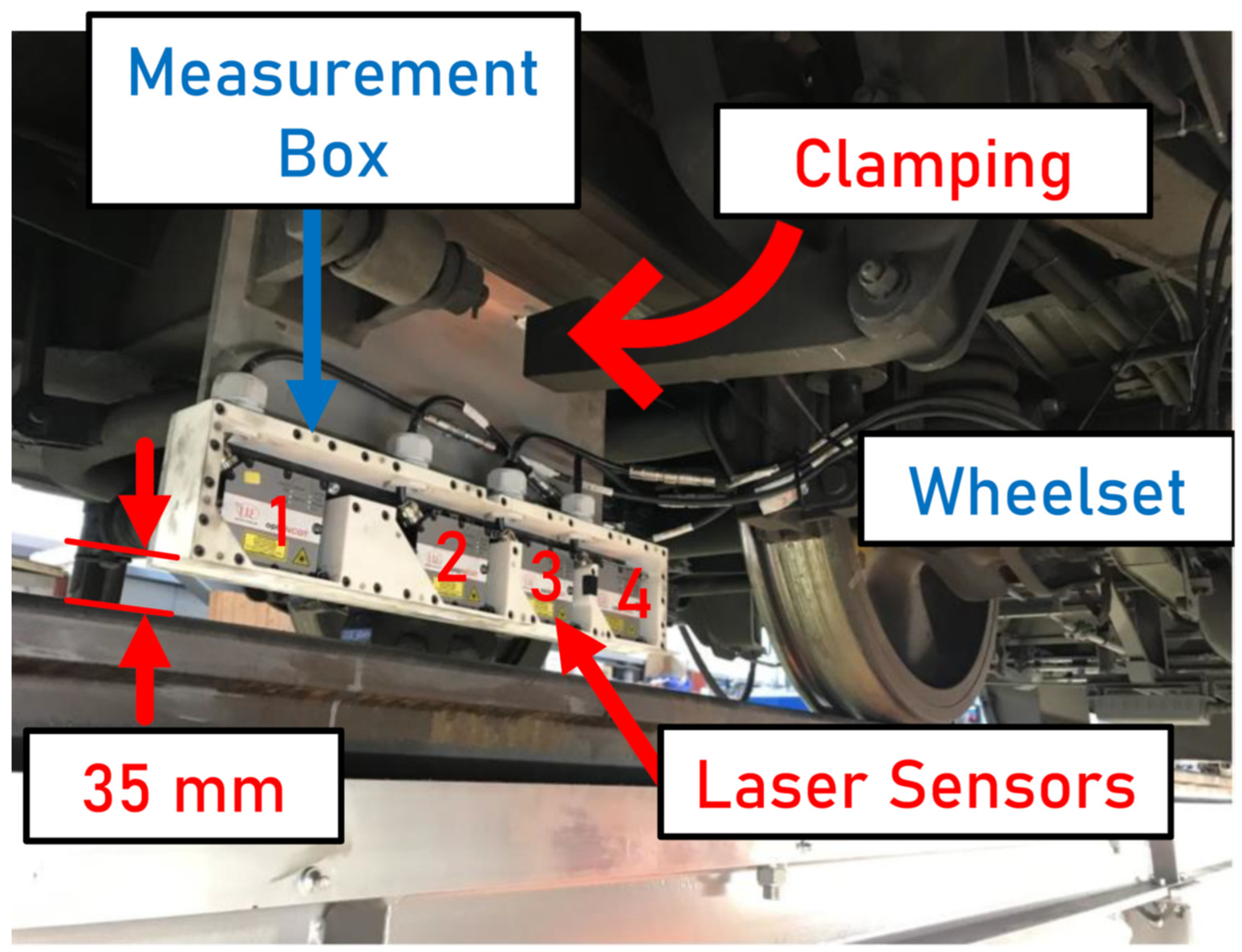
2.1. Setup

A measurement run was carried out with a test train from zb Zentralbahn AG between Stansstad and Engelberg. The line was a meter-gauge railway.

Table 1. Listing of the route for the measurements, including the reference sections and the toothed rack section inside the tunnel.

Kilometer	Location
2.69	Stansstad (Start)
11.28	Reference Section A
11.40	Reference Section B
18.60	Start Toothed Rack (Tunnel)
21.73	End Toothed Rack (Tunnel)
24.78	Engelberg (End)

shows an overview of the route characteristics.

The environmental conditions during the measurements were rain and snowfall. The rail surface outside the tunnel was mostly wet. The conditions of a dry rail surface were used for measurements in the tunnel section. Four Micro-Epsilon optoNCDT 2300-10LL laser triangulation sensors were used for the optical measurement of the distance between the rail surface and the sensor lens. The sensors provide a measuring range of $10 \mathrm{mm}$, a resolution of $0.15 \mathsf{\mu }\mathrm{m}$ and a reference distance of $35 \mathrm{mm}$. All four sensors were fixed on a steel plate. The distance values were recorded analogously via an NI 9222 module in a cRIO-9045 from National Instruments with a constant sampling frequency $f_S$ of $30 \mathrm{kHz}$. No encoder was used to trigger the measurement. The setup, including a protective box for the sensors, was clamped to the bogie of the train between the wheelsets. The sensors were protected from impacts and direct water sprays. The shielded cables were routed along the train into the passenger compartment. The lateral position of the measurement setup was set via clamping to the bogie frame. The measuring points were set to the center of the running surface. This setting was not changed any more during the measuring run. Due to the mounting on the bogie, the lateral adjustment over the running surface could not be changed, as no compensation mechanism was used. The distance between the sensor lenses and the rail surface was set to $35 \mathrm{mm}$ at standstill, which corresponded to the center of the measuring range of the sensor used at this sampling rate. The setup is shown in Figure 1.

The distances between the sensors were the following: $168 \mathrm{mm}$ (sensor 1 to 2), $113 \mathrm{mm}$ (sensor 2 to 3) and $105 \mathrm{mm}$ (sensor 3 to 4). The identical longitudinal distances between the sensors on the sensor plate were used in the laboratory experiments as described by Mauz et al. [18]. Four chord methods were evaluated, including their combination hereafter referenced as the optimized method. The acoustic roughness was calculated according to EN 15610 [20] and the supplements of Mauz et al. [21]. In the following, the limit spectrum of acoustic roughness according to EN ISO 3095 [22] is indicated for each comparison. The acoustic roughness was evaluated in the wavelength range between $3 \mathrm{mm}$ and $63 \mathrm{mm}$ in order to match the wavelength range of the reference measurement for comparison. The absolute deviation from the reference measurement was calculated for each one-third octave band at the corresponding wavelength $\lambda$. The mean deviation corresponded to an averaging over the entire wavelength range evaluated.

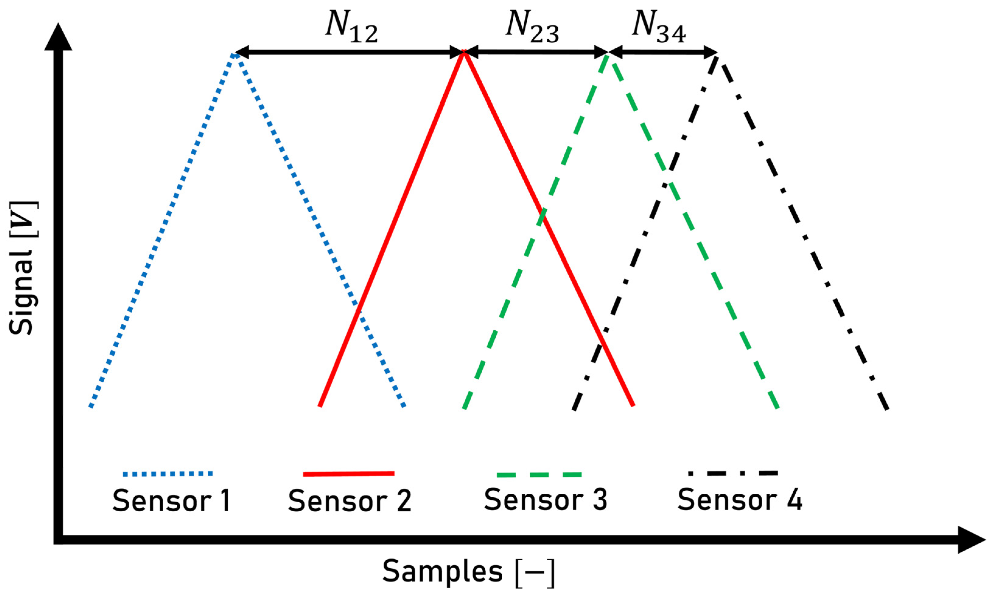
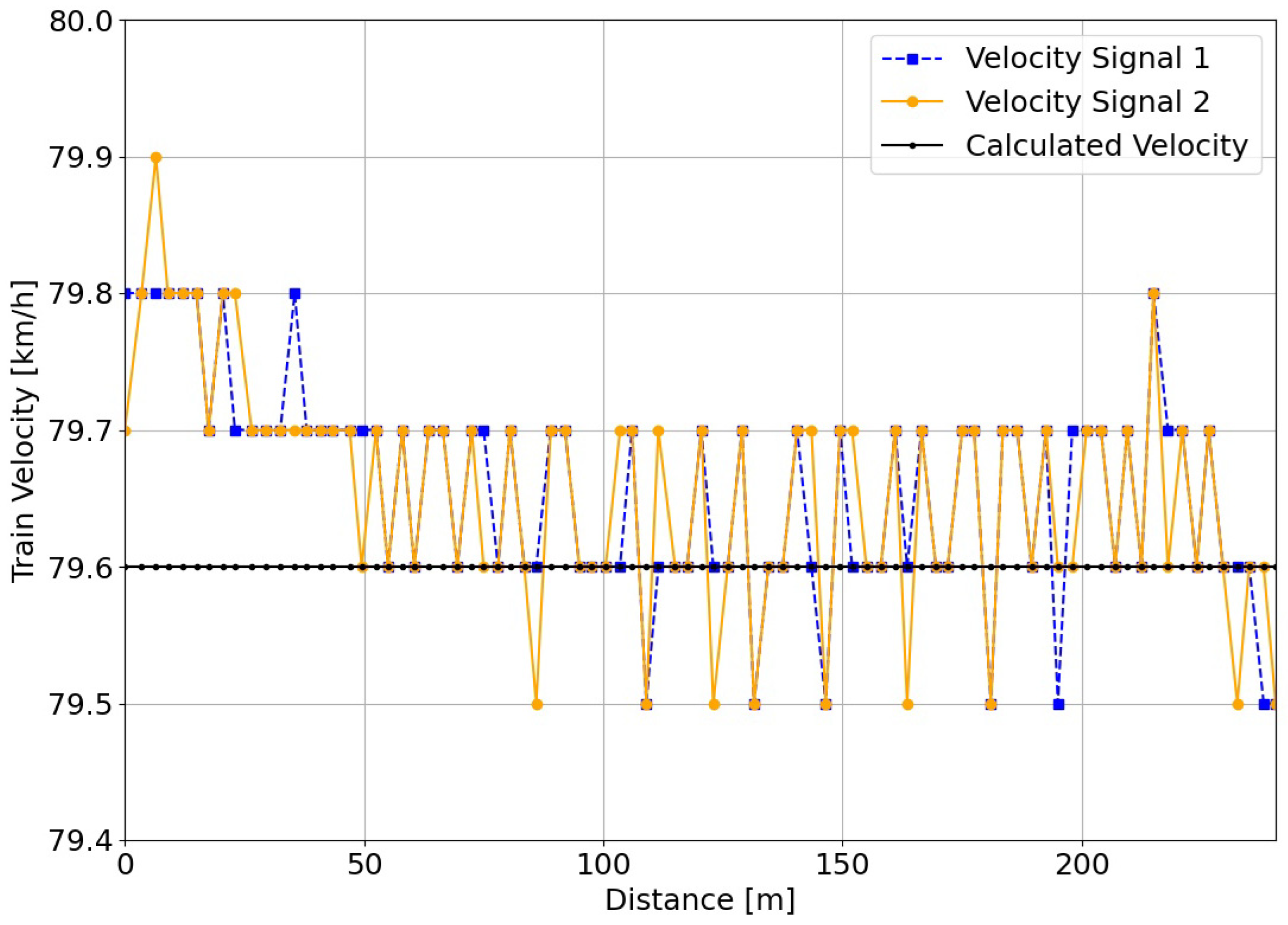
2.2. Velocity Calculation

To calculate the averaged sampling distance for individual segments of the measurement, the speed of the train must be known. This can be obtained from the known information on the sampling rate $f_S$ and the physical distance between the sensors $d$ by calculating the shift between two sensor signals. The velocity $v$ can be determined from the longitudinal distance $\Delta x$ and time distance $\Delta t$ between two corresponding data points:

$$v=\frac{\Delta x}{\Delta t}$$

(1)

The time interval between two corresponding data points is calculated by the known sampling frequency of the measurement:

$$\Delta t=\frac{1}{f_S}$$

(2)

The longitudinal distance $d$ between two sensors is defined by the chord structure and is known from the setup:

$$\Delta x=\frac{d}{N_x}$$

(3)

where $N_x$ represents the phase shift in the form of a number of data points. The shift between the sensor signals is shown in Figure 2.

The phase shift (number of data points) between the respective sensors is marked with the parameters $N_{12}$, $N_{23}$ and $N_{34}$. To determine the phase shift, the PCC (Phase Cross-Correlation) described by Schimmel [23] can be used, which was originally intended for an application in seismology. The basis is the theoretical assumption that all four sensors measure an identical profile on the same line with minor deviations to successfully achieve a correlation. Before determining the phase shift, the data are filtered with a high-pass filter to remove the long-wave components of the signals. If all known parameters are applied, this results in the velocity $v$:

$$v=\frac{f_S\cdot d}{N_x}$$

(4)

The velocity values calculated using this approach are verified with two on-board velocity recordings of the train.

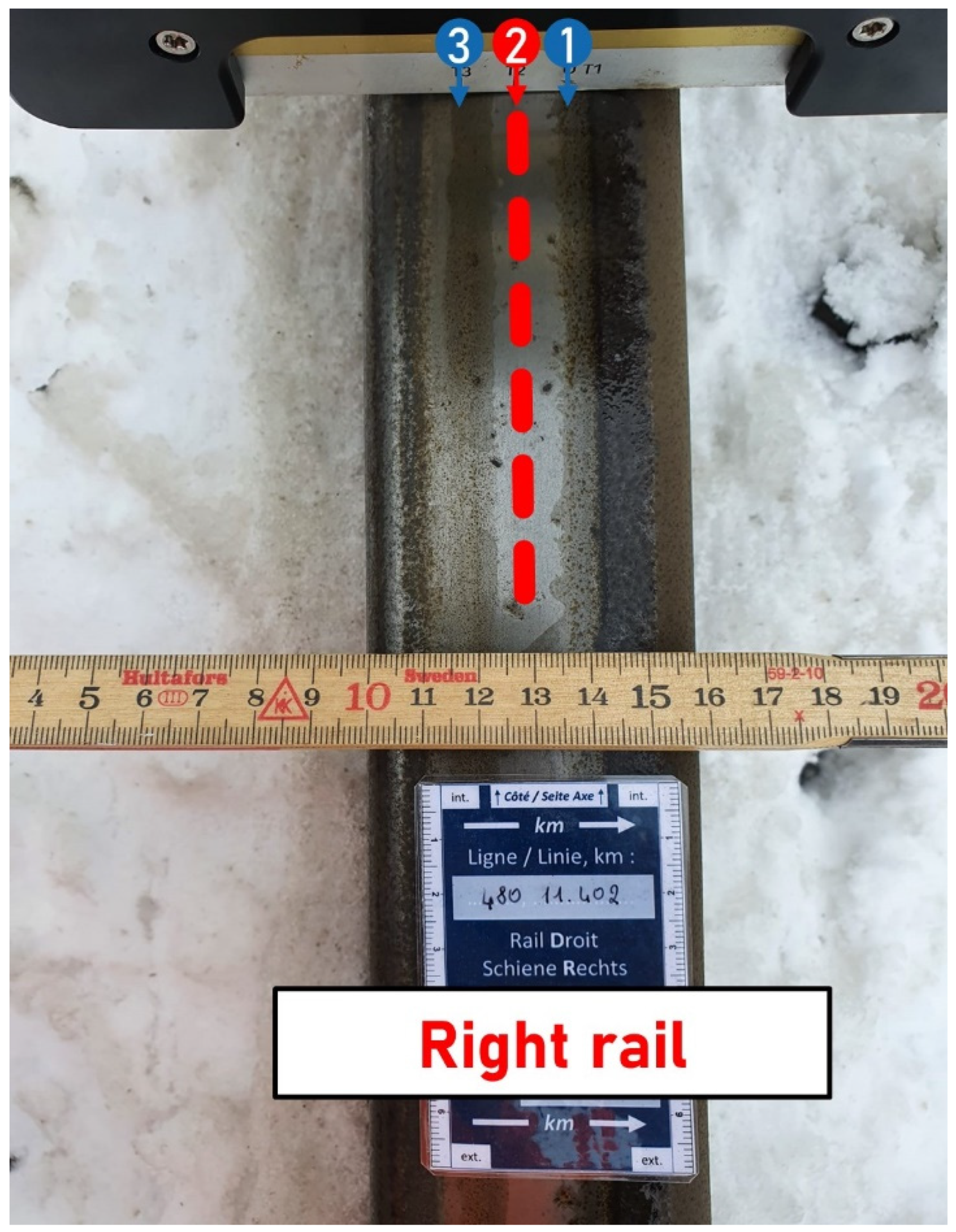
2.3. Reference Measurement

A tactile reference measurement was performed using an RM 150 HR instrument from Vogel & Plötscher. The device records the longitudinal rail profile over a length of $150 \mathrm{mm}$ per measurement with a measuring point distance of $0.1 \mathrm{mm}$. The profile was measured with three styli laterally shifted by $10 \mathrm{mm}$ to each other. With three measuring tracks, the state of the running surface could be measured depending on the lateral position. Relevant deviations in the spectra between the styli were to be expected depending on the surface conditions along the selected measuring track. A measuring resolution of $0.1 \mathsf{\mu }\mathrm{m}$ was achieved for the profile. The position of the measurement device on the rail is shown in Figure 3, including the three different measuring tracks.

The measurements were conducted and provided by SBB (Swiss Federal Railways). Reference measurements were taken at two sections at track position $11.282 \mathrm{km}$ (reference section A) and $11.402 \mathrm{km}$ (reference section B). The placement of non-destructive trigger marks was not appropriate, as these do not adhere to the rail surface for long on a track section in regular operation with higher train velocity on a straight section. Five measurements (segments) with a longitudinal distance of $3.6 \mathrm{m}$ from each other were taken per reference section and therefore provided an average of the acoustic roughness in this track section. The levels of the individual one-third octave bands $L_{1\dots 5}$ of the five measurements were averaged for each section. This resulted in a mean value $L_{avg}$ for each one-third octave band. The following root mean square value, which is based on EN 15610 [20], was used:

$$L_{avg}=10\cdot {\log }_{10}\left(\frac{{10}^{L_1/10}+{10}^{L_2/10}+{10}^{L_3/10}+{10}^{L_4/10}+{10}^{L_5/10}}{5}\right)$$

(5)

For the numerical comparison of the measured profile data with the reference measurements, the data from stylus 2 were used, as it was located in the center of the running surface. In addition, the profile data of styli 1 and 3 were evaluated to show a comparison for the shift in the lateral direction. The recorded profile data from the reference sections were processed in almost the same way as the data measured with the optical system. Instead of applying a pre-filter, the reference data were only detrended. The acoustic roughness was evaluated in the wavelength range between $3 \mathrm{mm}$ and $63 \mathrm{mm}$ due to the limited reference measuring length.

3. Results

3.1. Velocity Calculation

The train velocity was determined based on the measured laser sensor signals. The calculated velocity in the reference sections was $79.6{ \mathrm{km} \mathrm{h}}^{-1}$. The velocities recorded on-board the train varied between $79.5{ \mathrm{km} \mathrm{h}}^{-1}$ and $79.8{ \mathrm{km} \mathrm{h}}^{-1}$ or $79.9{ \mathrm{km} \mathrm{h}}^{-1}$ for velocity signal number two. The mean value was $79.66{ \mathrm{km} \mathrm{h}}^{-1}$ for velocity signal 1 and $79.65{ \mathrm{km} \mathrm{h}}^{-1}$ for velocity signal 2. Consequently, compared with the calculated velocity for the sections under consideration, there was a deviation of $0.06{ \mathrm{km} \mathrm{h}}^{-1}$ and $0.05{ \mathrm{km} \mathrm{h}}^{-1}$, respectively. The comparison of the results between the velocity measurements via the on-board measuring device of the train and the method for calculating the velocity based on the laser sensors is shown in Figure 4.

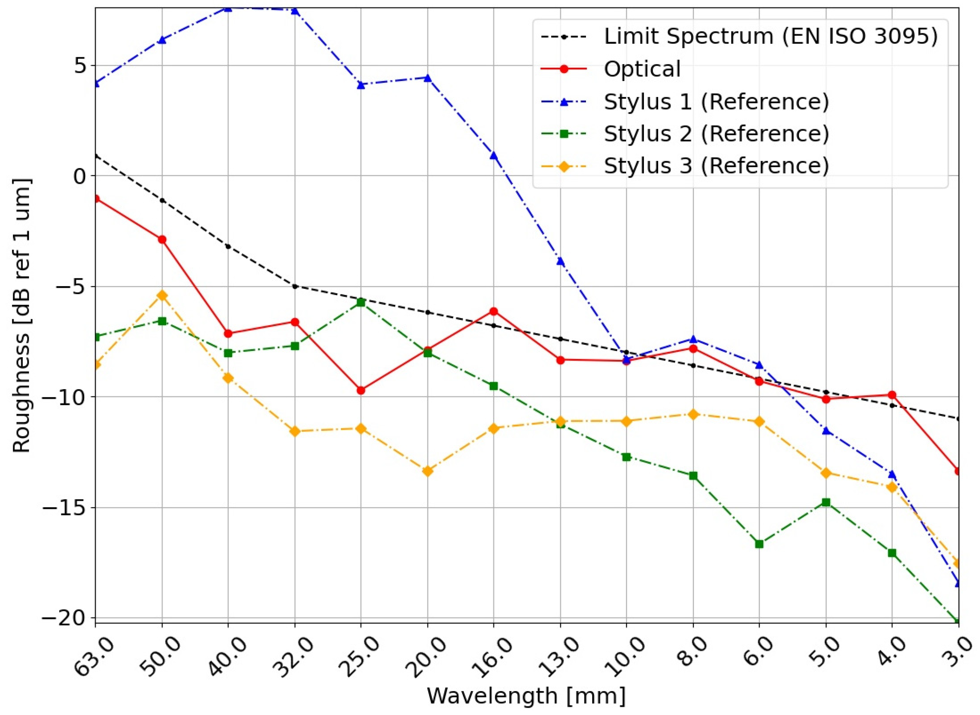
3.2. Reference Section Evaluation for SBB Measurement Data

The evaluation of the tactile reference measurements shows variations between the individual measurements. The deviations from the mean value for reference section B using the data from stylus 2 are stated in the following. Segment 4 shows the largest deviation of $12.96 \mathrm{dB}$ ($\lambda =63 \mathrm{mm})$. If this segment is not taken into account, the maximum deviations from the average vary between $4.96 \mathrm{dB}$(segment 1, $\lambda =32 \mathrm{mm}$) and $10.35 \mathrm{dB}$(segment 5, $\lambda =40 \mathrm{mm}$). The deviation averaged over the evaluated spectrum varies between $2.28 \mathrm{dB}$(segment 1) and $5.20 \mathrm{dB}$(segment 4). The spectrum of acoustic roughness for the five measurements of reference section B and the calculated average is shown in Figure 5. The spectrum of acoustic roughness for the five measurements of reference section A and the calculated average is shown in Figure A1.

3.3. Measurement with the Optical System in the Tunnel at $~40 km h^{-1}$

The route of the measurement run offered the possibility to measure in the tunnel and thus on a dry rail surface. The measurement was carried out at a mean speed of $39.5{ \mathrm{km} \mathrm{h}}^{-1}$ in the steep-toothed rack section. This resulted in a data point distance of $0.37 \mathrm{mm}$. Five adjacent segments with a respective length of $1 \mathrm{m}$ were measured. The five spectra were averaged according to Equation (5) for each one-third octave band to a mean value. The spectrum of acoustic roughness for reference section B is given for qualitative comparison of the measurement result in the tunnel. The evaluated acoustic roughness results of stylus 1 and 3 represent different lateral positions of the reference measurement. Between the reference sections and the beginning of the tunnel, there was a longitudinal difference of about $7 \mathrm{km}$. When comparing the average from five individual segments with reference section B, the average deviation over the evaluated spectrum was $3.61 \mathrm{dB}$. The deviation had a minimum value of $-3.96 \mathrm{dB}$ at a wavelength of $25 \mathrm{mm}$. The maximum deviation of $7.37 \mathrm{dB}$ occurred at a wavelength of $6 \mathrm{mm}$. The average deviation for the wavelength range between $3 \mathrm{mm}$ and $16 \mathrm{mm}$ was $5.30 \mathrm{dB}$. The spectrum of acoustic roughness for the measured section within the tunnel is shown in Figure 6. The spectrum of acoustic roughness for the measured section within the tunnel compared with reference section A is shown in Figure A2. The spectra of the five adjacent measurements used for the determination of the mean value are shown in Figure A5.

3.4. Measurement with the Optical System at $~50 km h^{-1}$

A measurement was performed on a section in front of the reference sections. The measurement was carried out at a mean speed of $48.6{ \mathrm{km} \mathrm{h}}^{-1}$. This resulted in a data point distance of $0.45 \mathrm{mm}$. Five adjacent segments with a respective length of $1 \mathrm{m}$ were measured. The five spectra were averaged according to Equation (5) for each one-third octave band to a mean value. The spectrum of acoustic roughness for reference section B is given for qualitative comparison of the measurement result. The measured section was located before the reference section. There was a relevant longitudinal offset to the reference sections. When comparing the average from five individual segments with reference section B, the average deviation over the evaluated spectrum was $1.48 \mathrm{dB}$. The deviation had a minimum value of $-2.51 \mathrm{dB}$ at a wavelength of $25 \mathrm{mm}$. The maximum deviation of $4.60 \mathrm{dB}$ occurred at a wavelength of $6 \mathrm{mm}$. The average deviation for the wavelength range between $3 \mathrm{mm}$ and $16 \mathrm{mm}$ was $2.55 \mathrm{dB}$. The spectrum of acoustic roughness for the measured section is shown in Figure 7. The spectrum of acoustic roughness for the measured section compared with reference section A is shown in Figure A3. The spectra of the five adjacent measurements used for the determination of the mean value are shown in Figure A6.

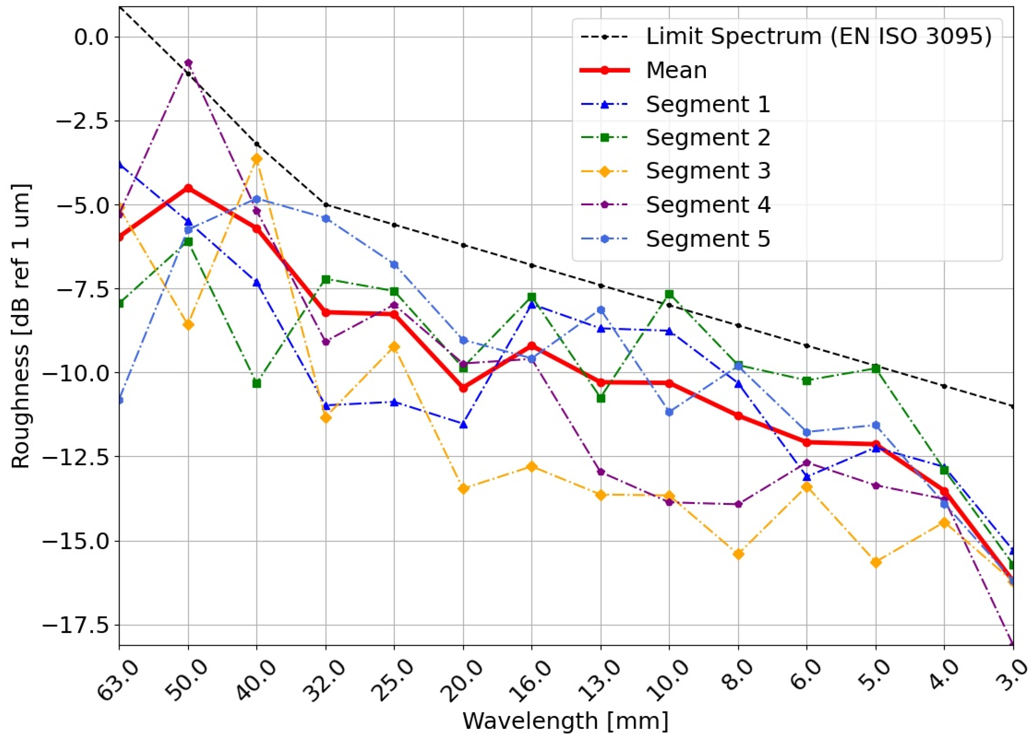
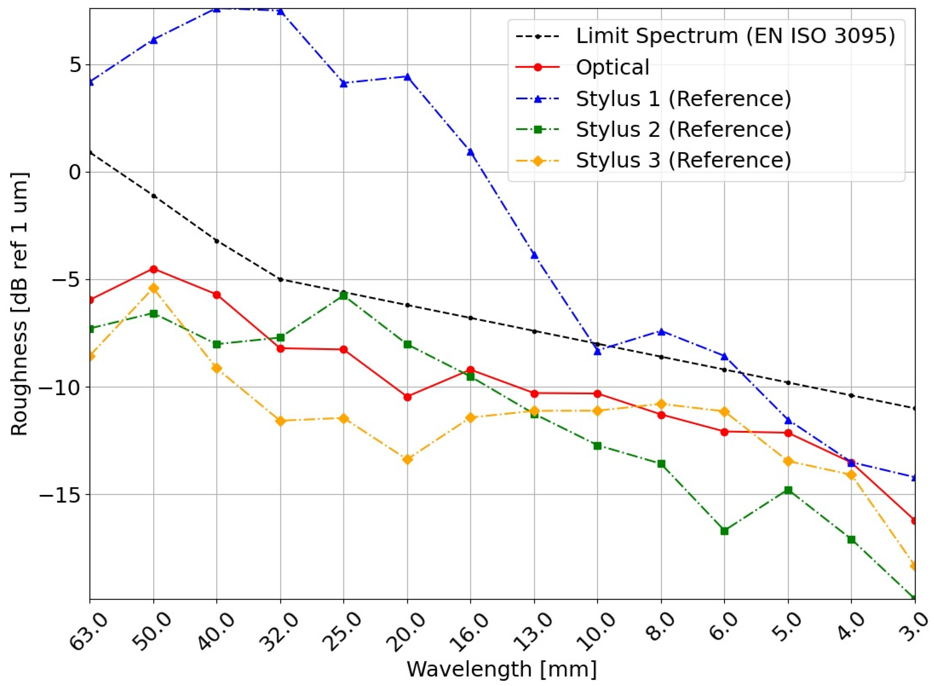
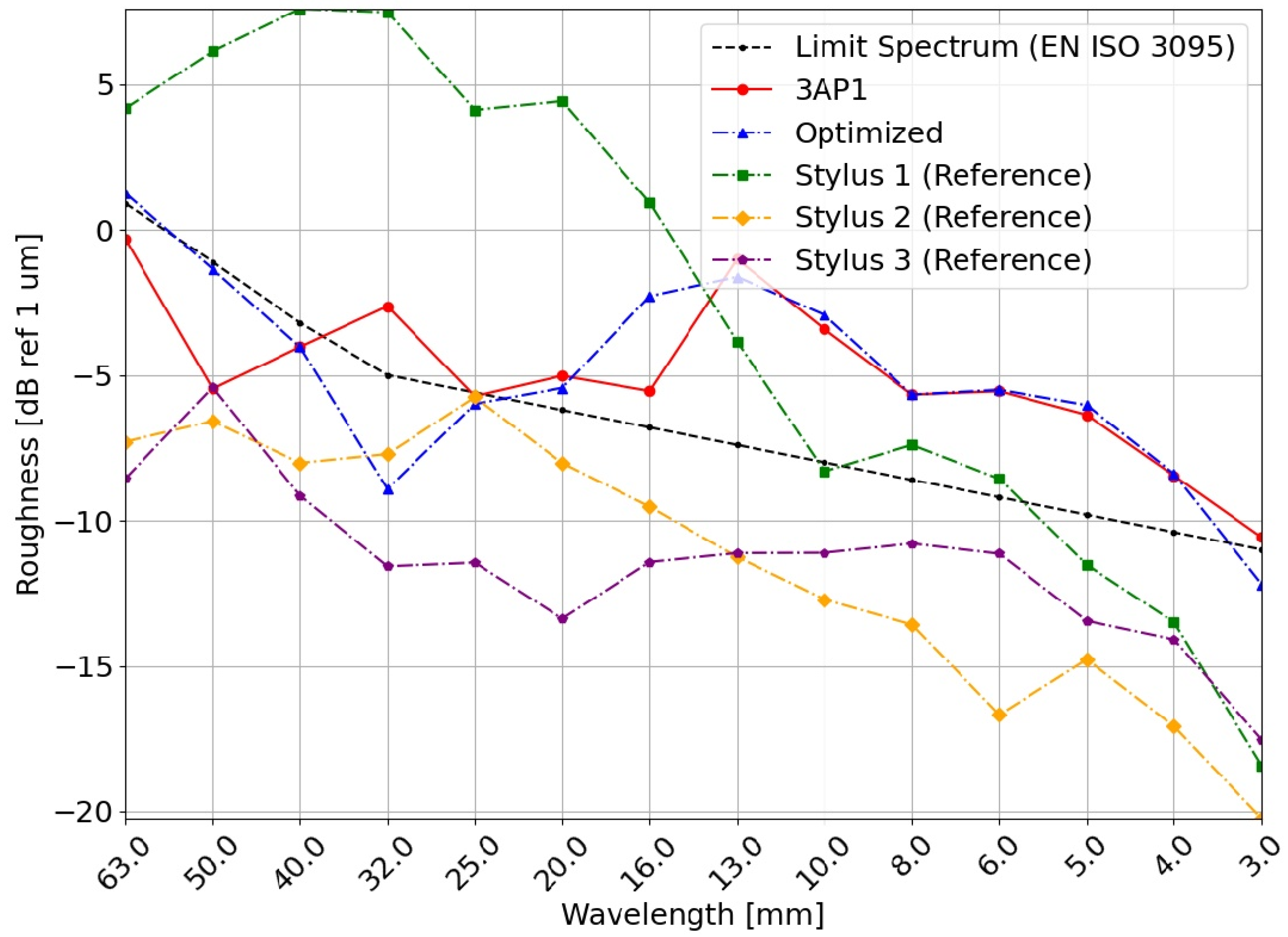
3.5. Measurement with the Optical System in the Reference Section $~80 km h^{-1}$

The single-chord method, the 3AP1 (Three-Point Asymmetrical 1) method, as described by Mauz et al. [18], was compared with the optimized method. The reference section was traversed with the calculated velocity of $79.6{ \mathrm{km} \mathrm{h}}^{-1}$. This resulted in a data point distance of $0.737 \mathrm{mm}$. A track length of $1 \mathrm{m}$ in wet conditions was taken into account for the evaluation. It was not possible to evaluate multiple adjacent segments because the raw data were distorted by outlier nests. For the single-chord method, a mean deviation from reference 2 of $6.39 \mathrm{dB}$ was determined. The deviation had a minimum of $0.03 \mathrm{dB}$ at a wavelength of $25 \mathrm{mm}$ and a maximum of $11.13$ dB at a wavelength of $6 \mathrm{mm}$. For the optimized method, the mean deviation from reference 2 was $6.44 \mathrm{dB}$. A minimum deviation of $-1.20 \mathrm{dB}$ for a wavelength of $32 \mathrm{mm}$ and a maximum deviation of $11.17 \mathrm{dB}$ for $6 \mathrm{mm}$ wavelength were obtained. If, in turn, only the wavelength range between $16 \mathrm{mm}$ and $63 \mathrm{mm}$ was taken into account for the comparison, the mean deviation would be reduced. For the single-chord method, the mean deviation from reference B was $3.45 \mathrm{dB}$. For the optimized method, the mean deviation was $3.74 \mathrm{dB}$. A comparable situation was obtained for test stand measurements with a wet rail, as experimentally illustrated by Mauz et al. [18]. The spectrum of acoustic roughness for a measured section compared with the reference section B is shown in Figure 8.

The spectrum of acoustic roughness for a measured section compared with reference section A is shown in Figure A4.

4. Discussion

The optical measurement concept showed promising results, especially for dry/drier rail sections measured at a speed of $40 {\mathrm{km} \mathrm{h}}^{-1}$ and $50{ \mathrm{km} \mathrm{h}}^{-1}$, respectively. For the wavelength range below $20 \mathrm{mm}$, an increasing deviation from the reference can be observed. These deviations increased for the measurement at $80 {\mathrm{km} \mathrm{h}}^{-1}$. The reasons for this could be the wet rail during the measurement and the influence of vehicle speed in the form of disturbances. Both influences could not be separated from each other at this point. To perform a comparison between optical measurement and a tactile reference in the wavelength range between $63 \mathrm{mm}$ and $250 \mathrm{mm}$, a longer measurement length of the tactile reference measurement would be required. The optical device performed continuous measurements and was therefore not limited in measuring length. For validation, a trolley device would be suitable.

The external disturbances of the train prevent the post-optimization of the measurement results because individual chords in the measurement setup are more disturbed than others. The lead sensor in the direction of travel failed before the tunnel section due to the wetness, which reduced the number of chords to one. The best results can be obtained in comparison with segment B of the reference section. Nevertheless, a lateral offset to stylus 2 as well as a longitudinal offset was expected, since no trigger marks were available. The spectra of stylus 1 and 3 represent the range of variation in the lateral direction. As the measurement on the reference section could only be carried out once, no information on the repeatability of the measurement system could be obtained.

Snow accumulation and wetness caused an influence on the measurement results. Due to increasing accumulations, the signal of the first sensor in the direction of travel was unreliable at the beginning of the tunnel section. Figure 9 shows the accumulations and the ambient conditions on the day of the measurement run.

Measurements with this optical measurement set-up should not take place under the described weather conditions. To keep the device operational between measurements, measures, as described by Zhou et al. [24], may be necessary. In addition, wetness created by the wheels of the train throwing snow and water caused further disturbances in the measuring system. This applies in particular to the first sensor in the direction of travel. Deviations in the measurements from the reference increased greatly in the wavelength range below 16 mm under the influence of wetness. In addition, there were clusters of outliers in the measured data set, which were not detected by the outlier removal and which distorted the spectrum of the acoustic roughness or shifted it to higher levels.

The measuring distance of $35 \mathrm{mm}$ between the sensor lenses and the top of the rail may be too small for regular use with other vehicles. Depending on the installed railway infrastructure, collisions can occur at this height. An example of this could be switches on a track with a toothed rack. In addition, the spring deflection of the primary suspension stage is often not known in detail and depends on the state of the loading of the vehicle. Based on the investigations of Liu et al. [25], a deflection in the range of $60 \mathrm{mm}$ to $70 \mathrm{mm}$ is to be expected. The sensor model used in this study had a measuring range of $10 \mathrm{mm}$. The limit of the measuring range is reached at points of interference that cause greater deflection, which can be obtained from the raw data. It is therefore recommended to use sensors with a higher measuring distance and a larger measuring range.

In the selected measurement setup, it was not possible to subsequently adjust the lateral position of the system during the current measuring ride. The hunting motion of the train on the track must be considered as a source of interference for the measurement. The frequency $f_h$ of this movement is described by the Klingel equation, as summarized by Knothe and Stichel [26]:

$$f_h=\frac{v}{2\pi }\cdot \sqrt{\frac{\delta }{e\cdot r}}$$

(6)

The speed $v$ of the train, the half track width $e$, the radius $r$ of the wheel as well as the equivalent conicity $\delta$ influence the frequency $f_h$. Since, in this study, a measurement on a meter gauge track was analyzed, a higher hunting motion frequency could be assumed compared with the $1435 \mathrm{mm}$ standard gauge.

The method for determining the velocity from the phase shift of the sensor signals to each other provides reliable values for selected segments. An advantage of this approach is that it does not require synchronization with measurement values from other sources, such as the velocity values recorded on-board the train. The sensor data are pre-filtered with a high pass filter. The short-wave components in the signal are especially suitable for determining the phase shift. Features such as local peaks in the signals can be successfully overlapped. Since four sensors in the setup measured the longitudinal profile, it was possible to calculate six different phase shifts and consequently six velocity values. No significant advantages could be determined in the comparison between small and larger sensor distances. The velocity value applied for the evaluation was calculated from the mean value of the six determined individual values.

The segment length set for the evaluation of the acoustic roughness determines the averaging of the acoustic roughness over the length. This length should not be chosen over several kilometers, as the rail surface condition within several kilometers can already deviate significantly. For measurements of the entire rail network, a standard length must therefore be defined for the evaluations to ensure comparability between the measurement results. Since the velocity is averaged for a selected data segment, distortions in the spectrum are to be expected here, since the velocity over a long segment deviates from the average value. The deviations shown in Figure 4 are small due to the choice of a straight rail segment and the evaluation of a short part of $240.5 \mathrm{m}$, but they could vary more for other parts of the route. Carrigan et al. [27] already demonstrated this distortion effect on the PSD (power spectral density) for measurements of axle-box accelerations.

According to the EN 15610 [20] standard, the longitudinal profile must be measured on three laterally displaced lines as long as the width of the running surface exceeds a value of $20 \mathrm{mm}$. If the width is less than $20 \mathrm{mm}$, it is only necessary to measure on one line in the middle of the running surface. It must therefore be investigated if a positioning system is sufficient or whether, alternatively, three identical systems must be used to measure the profile on three different laterally offset lines. In this study, the reference was recorded on a straight rail section. The influence of curves has not been investigated. Depending on the mounting position, curves can lead to a diagonal position of the measurement setup, which means that not all sensors measure at the same lateral position.

5. Conclusions and Outlook

An optical measurement system for measuring the acoustic roughness of rails was installed on a train. Measurements were performed at velocities up to $80{ \mathrm{km} \mathrm{h}}^{-1}$. Promising results were shown, especially for wavelengths above $16 \mathrm{mm}$ at a speed of $50{ \mathrm{km} \mathrm{h}}^{-1}$. The average deviation from the reference was $1.48 \mathrm{dB}$ for the entire wavelength range investigated at a speed of $50{ \mathrm{km} \mathrm{h}}^{-1}$. The velocity of the train could be reliably calculated based on the measured sensor data. The train speed calculated from the laser sensors deviated by only $0.06 {\mathrm{km} \mathrm{h}}^{-1}$ and $0.05 {\mathrm{km} \mathrm{h}}^{-1}$ from the average speed measured on the train. Even in difficult environmental conditions with snow and moisture on the rail, it was possible to perform exploitable measurements. However, it was shown that the quality of the results for one-third octave bands is not adequate at smaller wavelengths. The influence of wetness on the quality of the results in the wavelength range between $3 \mathrm{mm}$ and $16 \mathrm{mm}$ significantly increased the mean deviation from $3.45 \mathrm{dB}$(wavelength range from $16 \mathrm{mm}$ to $63 \mathrm{mm})$ to $6.44 \mathrm{dB}$(entire wavelength range) at a speed of $80{ \mathrm{km} \mathrm{h}}^{-1}$.

Further measurements should be carried out with a dry rail surface and at different speeds to determine the relevant influences for deviations in the spectrum. To improve performance at wavelengths below $16 \mathrm{mm}$, it is possible to reduce sensor distances by installing the sensors transversely to the direction of travel. This was not applied for these measurements due to the oval measuring point of the sensors. To correct dynamic influences, it is possible to install additional acceleration sensors which can remove vehicle dynamics from the measurement data. In addition, reproducibility should be investigated by measuring the same track section several times without extended intervals between the measurements. For this purpose, it is useful to have defined trigger marks to identify the measured segment more precisely. One possible approach could be to measure in parallel with a camera recording of the running surface and to flag the trigger marks optically. The measurement setup should therefore be supplemented by a camera. A camera can also be used to detect the lateral measurement position within the running surface. The influence of the lateral dynamics must be quantified and taken into account in the development of a positioning device. Liang et al. [28] developed a hunting motion compensation system that can operate up to a speed of $6{ \mathrm{km} \mathrm{h}}^{-1}$. For the investigated and larger measuring speeds, the requirements are consequently more demanding, and a new solution may have to be found.

References

1. Magiera, A.; Solecka, J. Environmental noise, its types and effects on health. Rocz. Panstw. Zakl. Hig. 2021, 72, 41–48. [Google Scholar] [CrossRef] [PubMed]
2. Zhang, L.; Ma, H. Investigation of Chinese residents’ community response to high-speed railway noise. Appl. Acoust. 2021, 172, 107615. [Google Scholar] [CrossRef]
3. Fiorini, C.V. Railway noise in urban areas: Assessment and prediction on infrastructure improvement combined with settlement development and regeneration in central Italy. Appl. Acoust. 2022, 185, 108413. [Google Scholar] [CrossRef]
4. Szwarc, M.; Kostek, B.; Kotus, J.; Szczodrak, M.; Czyżewski, A. Problems of Railway Noise-A Case Study. Int. J. Occup. Saf. Ergon. 2011, 17, 309–325. [Google Scholar] [CrossRef] [PubMed] [Green Version]
5. Polak, K.; Korzeb, J. Identification of the major noise energy sources in rail vehicles moving at a speed of 200 km/h. Energies 2021, 14, 3957. [Google Scholar] [CrossRef]
6. Thompson, D.J. On the Relationship between Wheel and Rail Surface Roughness and Rolling Noise. J. Sound Vib. 1996, 193, 149–160. [Google Scholar] [CrossRef]
7. Kuffa, M.; Ziegler, D.; Peter, T.; Kuster, F.; Wegener, K. A new grinding strategy to improve the acoustic properties of railway tracks. Proc. Inst. Mech. Eng. Part F J. Rail Rapid Transit 2018, 232, 214–221. [Google Scholar] [CrossRef]
8. Tufano, A.R.; Chiello, O.; Pallas, M.A.; Faure, B.; Chaufour, C.; Reynaud, E.; Vincent, N. On-Board Indirect Measurements of the Acoustic Quality of Railway Track: State-Of-The Art and Simulations. INTER-NOISE 2019 MADRID—48th International Congress Exhibition Noise Control Engineering, 2019. Available online: https://www.ingentaconnect.com/content/ince/incecp/2019/00000259/00000005/art00003 (accessed on 19 October 2022).
9. Grassie, S.L.; Saxon, M.J.; Smith, J.D. Measurement of longitudinal rail irregularities and criteria for acceptable grinding. J. Sound Vib. 1999, 227, 949–964. [Google Scholar] [CrossRef] [Green Version]
10. Tanaka, H.; Shimizu, A.; Sano, K. Development and verification of monitoring tools for realizing effective maintenance of rail corrugation. IET Conf. Publ. 2014, 2014, 14737938. [Google Scholar] [CrossRef]
11. Jeong, D.; Choi, H.S.; Choi, Y.J.; Jeong, W. Measuring acoustic roughness of a longitudinal railhead profile using a multi-sensor integration technique. Sensors 2019, 19, 1610. [Google Scholar] [CrossRef]
12. Lewis, R.B. Track-recording techniques used on British Rail. IEE Proc. B Electr. Power Appl. 1984, 131, 73–81. [Google Scholar] [CrossRef]
13. Bocciolone, M.; Caprioli, A.; Cigada, A.; Collina, A. A measurement system for quick rail inspection and effective track maintenance strategy. Mech. Syst. Signal Process. 2007, 21, 1242–1254. [Google Scholar] [CrossRef]
14. Carrigan, T.D.; Talbot, J.P. Extracting Information from Axle-Box Acceleration: On the Derivation of Rail Roughness Spectra in the Presence of Wheel Roughness. Notes Numer. Fluid Mech. Multidiscip. Des. 2021, 150, 286–294. [Google Scholar] [CrossRef]
15. Hauck, G.; Onnich, H.; Prögler, H. Entwicklung eines Messwagens zur Erfassung der Fahrgeräuschanhebungen durch Schienenriffeln. ETR Eisenb. Rundsch. 1997, 46, 153–159. [Google Scholar]
16. Kuijpers, A.H.W.M.; Schwanen, W.; Bongini, E. Indirect Rail Roughness Measurement: The ARRoW System within the LECAV Project. Notes Numer. Fluid Mech. Multidiscip. Des. 2012, 118, 563–570. [Google Scholar] [CrossRef]
17. Squicciarini, G.; Thompson, D.J.; Toward, M.G.R.; Cottrell, R.A. The effect of temperature on railway rolling noise. Proc. Inst. Mech. Eng. Part F J. Rail Rapid Transit 2015, 230, 1777–1789. [Google Scholar] [CrossRef] [Green Version]
18. Mauz, F.; Wigger, R.; Wahl, T.; Kuffa, M.; Wegener, K. Acoustic Roughness Measurement of Railway Tracks: Laboratory Investigation of External Disturbances on the Chord-Method with an Optical Measurement Approach. Appl. Sci. 2022, 12, 7732. [Google Scholar] [CrossRef]
19. Grassie, S.L. Measurement of railhead longitudinal profiles: A comparison of different techniques. WEAR Int. J. Sci. Technol. Frict. Lubr. Wear 1996, 191, 245–251. [Google Scholar] [CrossRef]
20. DIN EN 15610; Bahnanwendungen. Akustik. Messung der Schienen- und Radrauheit im Hinblick auf Die Entstehung von Rollgeräuschen. Deutsche Fassung. EN 15610:2019; Beuth Verlag: Berlin, Germany, 2021.
21. Mauz, F.; Wigger, R.; Wahl, T.; Kuffa, M.; Wegener, K. Acoustic roughness measurement of railway tracks: Implementation of an optical measurement approach & possible improvements to the standard. Proc. Inst. Mech. Eng. Part F J. Rail Rapid Transit 2022, 2022, 1210–1217. [Google Scholar] [CrossRef]
22. DIN EN ISO 3095; Akustik—Bahnanwendungen—Messung der Geräuschemission von Spurgebundenen Fahrzeugen (ISO 3095). Beuth Verlag: Berlin, Germany, 2013. [CrossRef]
23. Schimmel, M. Phase cross-correlations: Design, comparisons, and applications. Bull. Seismol. Soc. Am. 1999, 89, 1366–1378. [Google Scholar] [CrossRef]
24. Zhou, L.; Ding, L.; Yi, X. A review of snow melting and de-icing technologies for trains. Impact Factor 2022, 2022, 095440972110596. [Google Scholar] [CrossRef]
25. Liu, X.; Thompson, D.; Squicciarini, G.; Rissmann, M.; Bouvet, P.; Xie, G.; Martínez-Casas, J.; Carballeira, J.; Arteaga, I.L.; Garralaga, M.A.; et al. Measurements and modelling of dynamic stiffness of a railway vehicle primary suspension element and its use in a structure-borne noise transmission model. Appl. Acoust. 2021, 182, 108232. [Google Scholar] [CrossRef]
26. Knothe, K.; Stichel, S. Introduction to Lateral Dynamics of Railway Vehicles. In Rail Vehicle Dynamics; Springer International Publishing: Cham, Switzerland, 2017; pp. 159–168. ISBN 978-3-319-45376-7. [Google Scholar]
27. Carrigan, T.D.; Fidler, P.R.A.; Talbot, J.P. On the Derivation of Rail Roughness Spectra from Axle-box Vibration: Development of a New Technique. In Proceedings of the International Conference on Smart Infrastructure and Construction 2019 (ICSIC), Cambridge, UK, 8–10 July 2019; ICE Publishing: Cambridge, UK, 2019; Volume 2019, pp. 549–557. [Google Scholar]
28. Chen, L.; Li, Y.; Zhong, X.; Zheng, Q.; Liu, H. An Automated System for Position Monitoring and Correction of Chord-Based Rail Corrugation Measuring Points. IEEE Trans. Instrum. Meas. 2019, 68, 250–260. [Google Scholar] [CrossRef]
Figure 1. Experimental setup on the train with a measurement box, including four laser triangulation sensors (numbered 1 to 4) for distance measurements.
Applsci 12 11988 g001
Figure 2. The phase shift of the four-sensor setup.
Applsci 12 11988 g002
Figure 3. Tactile reference measurement on the right rail with the labelled positions of stylus 1, 2 and 3; image provided by SBB.
Applsci 12 11988 g003
Figure 4. Comparison of measured velocity (signal from the on-board equipment of the train) and velocity based on the PCC calculation and the measured data of the optical system.
Applsci 12 11988 g004
Figure 5. The spectrum of acoustic roughness for stylus 2 and reference section B (Mean), the five segments measured by SBB and the limit spectrum from EN ISO 3095 [22].
Applsci 12 11988 g005
Figure 6. Spectrum of acoustic roughness for measurement of the optical system in the tunnel, compared with reference section B and the limit spectrum from EN ISO 3095 [22].
Applsci 12 11988 g006
Figure 7. Spectrum of acoustic roughness for measurement of the optical system at 50   km   h 1 , compared with reference section B and the limit spectrum from EN ISO 3095 [22].
Applsci 12 11988 g007
Figure 8. Spectrum of acoustic roughness for measurement of the optical system near reference section B, compared with reference section B and the limit spectrum from EN ISO 3095 [22].
Applsci 12 11988 g008
Figure 9. Snow accumulation at the measuring box and driving in snow (snow cover thickness approx. 50   cm ).
Applsci 12 11988 g009