
Evaluating the Impact of Land Cover and Topography on Meteorological Parameters’ Relations and Similarities in the Alberta Oil Sands Region
 , , , and
Abstract
:1. Introduction
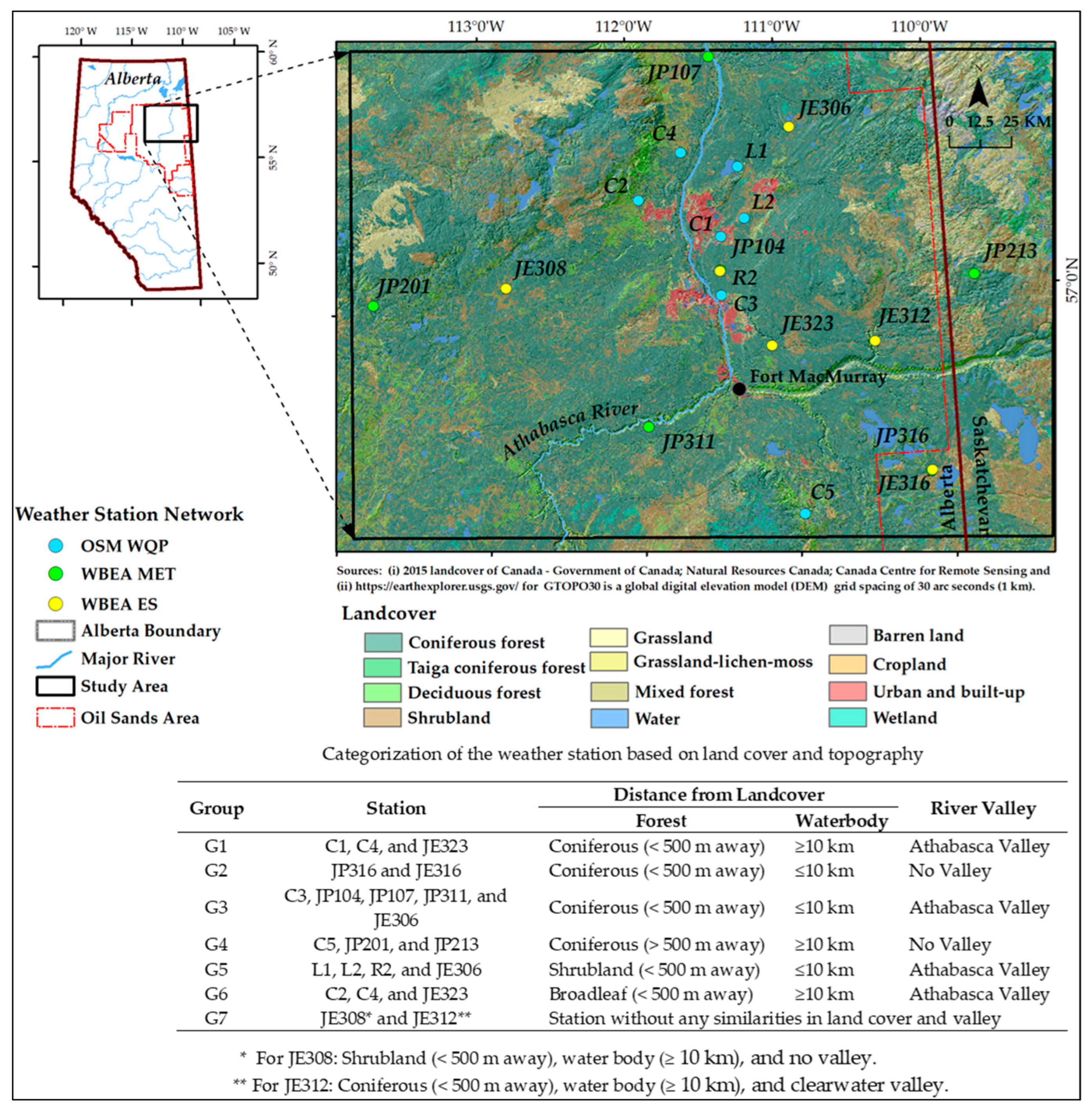
2. Study Area and Data Availability
3. Methods
3.1. Establishing Relationships for AT, RH, SR, BP, PR, and SD
3.2. Measures for WSD and WD
3.3. Similarity Analysis of Meteororlogical Parameters
- If D1-D2 is ±0.5 °C for AT, ±2.5 cm for SD, and ±5% for RH as per SOP’s recommendation.
- If the percentage deviation for D1 and D2 is ≤20% for hourly SR, 10% for daily SR, 1% for BP, and 2% for PR as per SOP’s recommendation. Here, we used the larger one between D1 and D2 in calculating the deviation. Notably, the larger one between D1 and D2 is used to compute the percentage deviation, and
- If D1-D2 is ±0.5 m/s (i.e., 1.8 km/h) for wind speed and ±5° for wind direction as per SOP’s recommendation.
4. Results
4.1. Relations and Similarity Analysis for AT, RH, SR, BP, PR, and SD
4.2. Similarity Analysis for WSD
4.3. Determining the Required Stations within Each Individual Group

| Group | Station ID | Network | Meteorological Parameter | ||||||
|---|---|---|---|---|---|---|---|---|---|
| AT | RH | SR | BP | PR | SD | WSD | |||
| G1 | C1 | OSM WQP | JE323 | ||||||
| C4 | JE323 | C1 | |||||||
| JE323 | WBEA ES | ||||||||
| G2 | JP316 | WBEA MT | |||||||
| JE316 | WBEA ES | JP316 | |||||||
| G3 | C3 | OSM WQP | JP104 | ||||||
| JP104 | WBEA MT | ||||||||
| JP107 | JP104 | ||||||||
| JP311 | JP104 | ||||||||
| JE306 | WBEA ES | JP104 | C3 | ||||||
| G4 | C5 | OSM WQP | JP213 | ||||||
| JP201 | WBEA MT | ||||||||
| JP213 | |||||||||
| G5 | L1 | OSM WQP | L2 | ||||||
| L2 | |||||||||
| R2 | WBEA ES | L2 | JE306 | ||||||
| JE306 | L2 | ||||||||
| G6 | C2 | OSM WQP | |||||||
| C4 | C2 | C2 | |||||||
| JE323 | WBEA ES | C2 | C2 | ||||||
| G7 | JE308 | WBEA ES | JE312 | ||||||
| JE312 | |||||||||
| Station is required to capture spatial variability in meteorological parameter | |
| AAA | Meteorological parameter shows at 70% similarity with station ‘AAA’ |
| There is no sensor for recording the meteorological parameter of interest |
5. Discussion
6. Conclusions
Author Contributions
Funding
Institutional Review Board Statement
Informed Consent Statement
Data Availability Statement
Acknowledgments
Conflicts of Interest
References
- World Meteorological Organization (WMO). Guide to Meteorological Instruments and Methods of Observation, 2018th ed.; World Meteorological Organization (WMO): Geneva, Switzerland, 2018. [Google Scholar]
- Borick, C.P.; Rabe, B.G. Weather or Not? Examining the Impact of Meteorological Conditions on Public Opinion Regarding Global Warming. Weather. Clim. Soc. 2014, 6, 413–424. [Google Scholar] [CrossRef]
- Hubbard, K.G. Spatial Variability of Daily Weather Variables in the High Plains of the USA. Agric. For. Meteorol. 1994, 68, 29–41. [Google Scholar] [CrossRef]
- Colston, J.M.; Ahmed, T.; Mahopo, C.; Kang, G.; Kosek, M.; de Sousa Junior, F.; Shrestha, P.S.; Svensen, E.; Turab, A.; Zaitchik, B. Evaluating Meteorological Data from Weather Stations, and from Satellites and Global Models for a Multi-Site Epidemiological Study. Environ. Res. 2018, 165, 91–109. [Google Scholar] [CrossRef]
- Mumtaz, R.; Baig, S.; Fatima, I. Analysis of Meteorological Variations on Wheat Yield and Its Estimation Using Remotely Sensed Data. A Case Study of Selected Districts of Punjab Province, Pakistan (2001-14). Ital. J. Agron. 2017, 12, 254–270. [Google Scholar] [CrossRef]
- Bahrami, M.; Shabani, A.; Mahmoudi, M.R.; Didari, S. Determination of Effective Weather Parameters on Rainfed Wheat Yield Using Backward Multiple Linear Regressions Based on Relative Importance Metrics. Complexity 2020, 2020, 1–10. [Google Scholar] [CrossRef]
- Schmiedeberg, C.; Schröder, J. Does Weather Really Influence the Measurement of Life Satisfaction? Soc. Indic. Res. 2014, 117, 387–399. [Google Scholar] [CrossRef]
- Liu, Z.; Yang, H.; Wei, X. Spatiotemporal Variation in Relative Humidity in Guangdong, China, from 1959 to 2017. Water 2020, 12, 3576. [Google Scholar] [CrossRef]
- Li, L.; Zha, Y. Mapping Relative Humidity, Average and Extreme Temperature in Hot Summer over China. Sci. Total Environ. 2018, 615, 875–881. [Google Scholar] [CrossRef] [PubMed]
- Shawky, M.; Moussa, A.; Hassan, Q.K.; El-Sheimy, N. Performance Assessment of Sub-Daily and Daily Precipitation Estimates Derived from GPM and GSMaP Products over an Arid Environment. Remote Sens. 2019, 11, 2840. [Google Scholar] [CrossRef] [Green Version]
- Hubbard, K.G.; Hollinger, S.E. Standard Meteorological Measurements. In Micrometeorology in Agricultural Systems, Volume 47; Hatfield, J.L., Baker, J.M., Eds.; The American Society of Agronomy, Crop Science Society of America, and Soil Science Society of America: Madison, WI, USA, 2005; pp. 1–30. [Google Scholar]
- Wang, L.; Kisi, O.; Zounemat-Kermani, M.; Salazar, G.A.; Zhu, Z.; Gong, W. Solar Radiation Prediction Using Different Techniques: Model Evaluation and Comparison. Renew. Sustain. Energy Rev. 2016, 61, 384–397. [Google Scholar] [CrossRef]
- Lledó, L.; Torralba, V.; Soret, A.; Ramon, J.; Doblas-Reyes, F.J. Seasonal Forecasts of Wind Power Generation. Renew. Energy 2019, 143, 91–100. [Google Scholar] [CrossRef]
- WMO. Guide to Meteorological Instruments and Methods of Observation, 2010th ed.; World Meteorological Organization (WMO): Geneva, Switzerland, 2010. [Google Scholar]
- World Meteorological Organization (WMO). Manual on the Global Observing System; WMO: Geneva, Switzerland, 2017; p. 172. [Google Scholar]
- World Meteorological Organization (WMO). Manual on the Global Data-Processing and Forecasting System; WMO: Geneva, Switzerland, 2012; p. 193. [Google Scholar]
- Government of Alberta. Oil Sands Facts and Statistics. Available online: https://www.alberta.ca/oil-sands-facts-and-statistics.aspx (accessed on 21 April 2021).
- Papineau, J.W.; Deacon, L. Fort McMurray and the Canadian Oil Sands: Local Coverage of National Importance. Environ. Commun. 2017, 11, 593–608. [Google Scholar] [CrossRef]
- Ahmed, M.R.; Rahaman, K.R.; Hassan, Q.K. Remote Sensing of Wildland Fire-Induced Risk Assessment at the Community Level. Sensors 2018, 18, 1570. [Google Scholar] [CrossRef] [PubMed] [Green Version]
- Hatfield Consultants. Regional Aquatics Monitoring in Support of the Joint Oil Sands Monitoring Plan: Final 2015 Program Report; Hatfield Consultants: Vancouver, BC, Canada, 2016. [Google Scholar]
- Wood Buffalo Environmental Association (WBEA). Forest METEOROLOGICAL TOWER DATA. Available online: https://wbea.org/deposition/forest-meteorological-tower-data/ (accessed on 10 July 2022).
- Deshmukh, D.; Ahmed, M.R.; Dominic, J.A.; Zaghloul, M.S.; Gupta, A.; Achari, G.; Hassan, Q.K. Quantifying Relations and Similarities of the Meteorological Parameters among the Weather Stations in the Alberta Oil Sands Region. PLoS ONE 2022, 17, e0261610. [Google Scholar] [CrossRef] [PubMed]
- Deshmukh, D.; Ahmed, M.R.; Dominic, J.A.; Gupta, A.; Achari, G.; Hassan, Q.K. Suitability Assessment of Weather Networks for Wind Data Measurements in the Athabasca Oil Sands Area. Climate 2022, 10, 10. [Google Scholar] [CrossRef]
- Baldocchi, D.; Ma, S. How Will Land Use Affect Air Temperature in the Surface Boundary Layer? Lessons Learned from a Comparative Study on the Energy Balance of an Oak Savanna and Annual Grassland in California, USA. Tellus Ser. B Chem. Phys. Meteorol. 2013, 65, 20. [Google Scholar] [CrossRef] [Green Version]
- Tsintikidis, D.; Georgakakos, K.P.; Sperfslage, J.A.; Smith, D.E.; Carpenter, T.M. Precipitation Uncertainty, Raingauge Network Design within Folsom Lake Watershed. J. Hydrol. Eng. 2002, 7, 175–184. [Google Scholar] [CrossRef]
- Vajda, A.; Venäläinen, A. The Influence of Natural Conditions on the Spatial Variation of Climate in Lapland, Northern Finland. Int. J. Climatol. 2003, 23, 1011–1022. [Google Scholar] [CrossRef]
- Ruel, J.C.; Pin, D.; Cooper, K. Effect of Topography on Wind Behaviour in a Complex Terrain. Forestry 1998, 71, 261–265. [Google Scholar] [CrossRef] [Green Version]
- Cohen-Zada, A.L.; Maman, S.; Blumberg, D.G. Earth Aeolian Wind Streaks: Comparison to Wind Data from Model and Stations. J. Geophys. Res. Planets 2017, 122, 1119–1137. [Google Scholar] [CrossRef]
- López-Espinoza, E.D.; Zavala-Hidalgo, J.; Mahmood, R.; Gómez-Ramos, O. Assessing the Impact of Land Use and Land Cover Data Representation on Weather Forecast Quality: A Case Study in Central Mexico. Atmosphere 2020, 11, 1242. [Google Scholar] [CrossRef]
- Dorji, U.; Olesen, J.E.; Bøcher, P.K.; Seidenkrantz, M.S. Spatial Variation of Temperature and Precipitation in Bhutan and Links to Vegetation and Land Cover. Mt. Res. Dev. 2016, 36, 66–79. [Google Scholar] [CrossRef] [Green Version]
- Li, J.; Zheng, X.; Zhang, C.; Chen, Y. Impact of Land-Use and Land-Cover Change on Meteorology in the Beijing-Tianjin-Hebei Region from 1990 to 2010. Sustainability 2018, 10, 176. [Google Scholar] [CrossRef] [Green Version]
- Magnago, L.F.S.; Rocha, M.F.; Meyer, L.; Martins, S.V.; Meira-Neto, J.A.A. Microclimatic Conditions at Forest Edges Have Significant Impacts on Vegetation Structure in Large Atlantic Forest Fragments. Biodivers. Conserv. 2015, 24, 2305–2318. [Google Scholar] [CrossRef]
- Oliver, T.H.; Morecroft, M.D. Interactions between Climate Change and Land Use Change on Biodiversity: Attribution Problems, Risks, and Opportunities. Wiley Interdiscip. Rev. Clim. Chang. 2014, 5, 317–335. [Google Scholar] [CrossRef] [Green Version]
- Nahian, M.R.; Nazem, A.; Nambiar, M.K.; Byerlay, R.; Mahmud, A.S.; Seguin, A.M.; Robe, F.R.; Ravenhill, J.; Aliabadi, A.A. Complex Meteorology over a Complex Mining Facility: Assessment of Topography, Land Use, and Grid Spacing Modifications in WRF. J. Appl. Meteorol. Climatol. 2020, 59, 769–789. [Google Scholar] [CrossRef]
- Baltas, E.A.; Mimikou, M.A. GIS-Based Optimisation of the Hydrometeorological Network in Greece. Int. J. Digit. Earth 2009, 2, 171–185. [Google Scholar] [CrossRef]
- Yildirim, V.; Nisanci, R.; Husniye, E.; Yildiz, C.; Yildiz, O. A GIS-Based Siting Technique for Automatic Weather Stations in Trabzon, Turkey. Weather 2016, 71, 43–49. [Google Scholar] [CrossRef]
- Rojas Briceño, N.B.; Salas López, R.; Silva López, J.O.; Oliva-Cruz, M.; Gómez Fernández, D.; Terrones Murga, R.E.; Iliquín Trigoso, D.; Barrena Gurbillón, M.; Barboza, E. Site Selection for a Network of Weather Stations Using AHP and Near Analysis in a GIS Environment in Amazonas, NW Peru. Climate 2021, 9, 169. [Google Scholar] [CrossRef]
- Alejo, L.A. Suitability Analysis for Optimum Network of Agrometeorological Stations: A Case Study of Visayas Region, Philippines. J. Agrometeorol. 2018, 20, 269–274. [Google Scholar] [CrossRef]
- Eichenlaub, V.L. Lakes, Effects on Climate. In Climatology. Encyclopedia of Earth Science; Springer: Boston, MA, USA, 1987; pp. 1–18. [Google Scholar] [CrossRef]
- Ratner, B. The Correlation Coefficient: Its Values Range between 1/−1, or Do They? J. Target. Meas. Anal. Mark. 2009, 17, 139–142. [Google Scholar] [CrossRef] [Green Version]
- Ghorbani, M.A.; Mahmoud Alilou, S.; Javidan, S.; Naganna, S.R. Assessment of Spatio-Temporal Variability of Rainfall and Mean Air Temperature over Ardabil Province, Iran. SN Appl. Sci. 2021, 3, 10. [Google Scholar] [CrossRef]
- Willmott, C.J.; Matsuura, K. Advantages of the Mean Absolute Error (MAE) over the Root Mean Square Error (RMSE) in Assessing Average Model Performance. Clim. Res. 2005, 30, 79–82. [Google Scholar] [CrossRef]
- WorleyParsons Canada. Groundwater Flow Model for the Athabasca Oil Sands, North of Fort MacMurray: Phase 1 Conceptual and Numerical Model Development; WorleyParsons Canada: Burnaby, BC, Canada, 2012. [Google Scholar]
- Audet, P.; Pinno, B.D.; Thiffault, E. Reclamation of Boreal Forest after Oil Sands Mining: Anticipating Novel Challenges in Novel Environments. Can. J. For. Res. 2015, 45, 364–371. [Google Scholar] [CrossRef] [Green Version]
- Suncor Energy Inc. Appendix 3: Climate Change in the Oil Sands Region; Suncor Energy Inc.: Edmonton, AB, Canada, 2007. [Google Scholar]
- Apogee Instruments. Affordable and Accurate Barometric Pressure Sensor. Available online: https://www.apogeeinstruments.com/barometric-pressure (accessed on 21 April 2021).
- Government of Alberta. Environmental Quality Assurance–Standards and Protocols. Available online: https://www.alberta.ca/environmental-quality-assurance-standards-and-protocols.aspx (accessed on 21 April 2021).
- Hinckley, A. Pyranometers: What You Need to Know. Available online: https://www.campbellsci.com/blog/pyranometers-need-to-know (accessed on 21 April 2021).
- World Meteorological Organization (WMO). Guide to Instruments and Methods of Observation, 2021th ed.; World Meteorological Organization (WMO): Geneva, Switzerland, 2021. [Google Scholar]
- Sekhon, N.S.; Hassan, Q.K.; Sleep, R.W. Evaluating Potential of MODIS-Based Indices in Determining “Snow Gone” Stage over Forest-Dominant Regions. Remote Sens. 2010, 2, 1348–1363. [Google Scholar] [CrossRef] [Green Version]
- Akther, M.S.; Hassan, Q.K. Remote Sensing Based Estimates of Surface Wetness Conditions and Growing Degree Days over Northern Alberta, Canada. Boreal Environ. Res. 2011, 16, 407–416. [Google Scholar]
- Hassan, Q.K.; Bourque, C.P.A.; Meng, F.R. Estimation of Daytime Net Ecosystem CO2 Exchange over Balsam Fir Forests in Eastern Canada: Combining Averaged Tower-Based Flux Measurements with Remotely Sensed MODIS Data. Can. J. Remote Sens. 2006, 32, 405–416. [Google Scholar] [CrossRef] [Green Version]
- Ejiagha, I.R.; Ahmed, M.R.; Dewan, A.; Gupta, A.; Rangelova, E.; Hassan, Q.K. Urban Warming of the Two Most Populated Cities in the Canadian Province of Alberta, and Its Influencing Factors. Sensors 2022, 22, 2894. [Google Scholar] [CrossRef]
- Wood Buffalo Environmental Association (WBEA). Annual Report 2019; Wood Buffalo Environmental Association (WBEA): Fort McMurray, AB, Canada, 2020. [Google Scholar]
- Bowditch, N. The Weather Elements. In American Practical Navigator; National Geospatial-Intelegence Agency: Sringfield, VA, USA, 2017; pp. 603–635. [Google Scholar]
- O’Hare, G.; Sweeney, J.; Wilby, R. Weather, Climate and Climate Change: Human Perspective; Routledge: New York, NY, USA, 2013. [Google Scholar]

| Group | Station Pair | Comparison | Common Meteorological Parameter | Common Data Period | ||
|---|---|---|---|---|---|---|
| Height (m) | Scale | From | To | |||
| G1 | C1 vs. C4 | 2 and 10 * | daily | AT, RH, SR, PR SD, and WSD | 25-July-2011 | 31-March-2017 |
| C1 vs. JE323 | 2 | daily | AT, RH, and SR | 15-March-2014 | 31-March-2017 | |
| C4 vs. JE323 | AT, RH, SR, and BP | 15-March-2014 | 31-March-2017 | |||
| G2 | JP316 vs. JE316 | 2 | hourly | AT, RH, SR, and WSD | 11-April-2014 | 01-April-2018 |
| G3 | C3 vs. JE306 | 2 | daily | AT, RH, SR, and BP | 25-March-2014 | 31-March-2017 |
| C3 vs. JP104 | AT, RH, and SR | 30-May-2014 | 31-March-2017 | |||
| C3 vs. JP107 | AT, RH, SR, and PR | 29-August-2012 | 31-March-2017 | |||
| C3 vs. JP311 | AT, RH, SR, and PR | 30-May-2014 | 31-March-2017 | |||
| JP 104 vs. JE306 | hourly | AT, RH, and SR WD | 30-May-2014 03-September-2014 | 31-January-2019 31-January-2019 | ||
| JP 107 vs. JE306 | AT, RH, and SR WSD | 01-May-2014 03-September-2014 | 01-April-2018 01-April-2018 | |||
| JP 311 vs. JE306 | AT, RH, and SR WSD | 25-March-2014 03-September-2014 | 01-April-2018 01-April-2018 | |||
| JP 104 vs. JP107 | 2, 16, 21, and 29 | hourly | AT, RH, SR, and WSD | 30-May-2014 | 01-April-2018 | |
| JP 104 vs. JP311 | AT, RH, SR, and WSD | 30-May-2014 | 01-April-2018 | |||
| JP 107 vs. JP311 | AT, RH, SR, and WSD | 30-July-2013 | 01-April-2018 | |||
| G4 | C5 vs. JP201 | 2 | daily | AT, RH, and SR | 27-May-2014 | 31-March-2017 |
| C5 vs. JP213 | AT, RH, SR, and PR | 18-July-2012 | 31-March-2017 | |||
| JP201 vs. JP213 | 2, 16, 21, and 29 | hourly | AT, RH, SR, and WSD | 03-September-2014 27-May-2014 | 01-April-2018 01-April-2018 | |
| G5 | L1 vs. L2 | 2 | daily | AT and RH PR | 25-September-2007 01-August-2008 | 31-March-2017 31-March-2017 |
| L1 vs. R2 | AT and RH | 24-January-2011 | 02-January-2016 | |||
| L2 vs. R2 | ||||||
| L1 vs. JE306 | 2 | daily | AT and RH | 25-March-2014 | 31-March-2017 | |
| L2 vs. JE306 | ||||||
| R2 vs. JE306 | 2 | hourly | AT, RH, SR, and BP WSD | 25-March-2014 01-January-2015 | 01-April-2019 01-April-2019 | |
| G6 | C2 vs. C4 | 2 and 10 * | daily | AT, RH, SR, BP, PR SD, and WSD | 25-July-2011 | 31-March-2017 |
| C2 vs. JE323 | 2 | daily | AT, RH, SR, and BP | 15-March-2014 | 31-March-2017 | |
| C4 vs. JE323 | ||||||
| G7 | JE308 vs. JE312 | 2 | hourly | AT, RH, SR, and BP WSD | 25-March-2014 03-September-2014 | 01-April-2019 31-March-2019 |
| Met. Parameter | Measure | Group | |||||||||
|---|---|---|---|---|---|---|---|---|---|---|---|
| G1 | G2 | G4 | |||||||||
| * C1 vs. C4 | * C1 vs. JE323 | * C4 vs. JE323 | * JP316 vs. JE316 | * C5 vs. JP201 | * C5 vs. JP213 | * JP201 vs. JP213 | ** JP201 vs. JP213 | ^ JP201 vs. JP213 | ^^ JP201 vs. JP213 | ||
| AT | n | 2076 | 1112 | 1112 | 32,736 | 1035 | 1607 | 30,758 | 33,282 | 29,601 | 32,783 |
| AAE (°C) | 1.16 | 2.49 | 1.82 | 1.31 | 1.82 | 3.92 | 4.27 | 2.65 | 2.44 | 2.36 | |
| r | 1.00 | 0.99 | 0.99 | 0.99 | 0.99 | 0.68 | 0.72 | 0.97 | 0.97 | 0.98 | |
| PS (%) | 53.76 | 22.75 | 32.55 | 55.97 | 29.08 | 28.44 | 24.18 | 26.47 | 28.35 | 29.47 | |
| RH | n | 2076 | 1112 | 1112 | 32,737 | 1035 | 1711 | 33,064 | 33,284 | 29,601 | 32,327 |
| AAE (%) | 5.76 | 5.04 | 5.08 | 4.81 | 8.16 | 6.66 | 9.68 | 9.57 | 9.39 | 9.47 | |
| r | 0.88 | 0.93 | 0.88 | 0.93 | 0.69 | 0.81 | 0.74 | 0.77 | 0.78 | 0.78 | |
| PS (%) | 83.00 | 87.68 | 87.32 | 86.87 | 73.33 | 79.02 | 68.34 | 66.36 | 67.1 | 66.71 | |
| SR | n | 2076 | 1112 | 1112 | 21,511 | 1035 | 1710 | 25,402 | - | - | - |
| AAE (W/m2) | 16.41 | 29.74 | 37.18 | 59.77 | 24.69 | 22.71 | 63.39 | - | - | - | |
| r | 0.97 | 0.88 | 0.85 | 0.92 | 0.93 | 0.93 | 0.85 | - | - | - | |
| PS (%) | 32.38 | 24.85 | 21.12 | 30.81 | 26.98 | 32.12 | 27.30 | - | - | - | |
| BP | n | - | - | 1112 | - | - | - | - | - | - | - |
| AAE (kPa) | - | - | 1.82 | - | - | - | - | - | - | - | |
| r | - | - | 0.98 | - | - | - | - | - | - | - | |
| PS (%) | - | - | 0.00 | - | - | - | - | - | - | - | |
| PR | n | 2002 | - | - | - | - | 1710 | - | - | - | - |
| AAE (mm) | 0.92 | - | - | - | - | 22.71 | - | - | - | - | |
| r | 0.69 | - | - | - | - | 0.93 | - | - | - | - | |
| PS (%) | 8.85 | - | - | - | - | 32.12 | - | - | - | - | |
| SD | n | 2076 | - | - | - | - | - | - | - | - | - |
| AAE (cm) | 2.83 | - | - | - | - | - | - | - | - | - | |
| r | 0.95 | - | - | - | - | - | - | - | - | - | |
| PS (%) | 76.40 | - | - | - | - | - | - | - | - | - | |
| Met. Parameters | Measures | G3 | ||||||||||||||||||
|---|---|---|---|---|---|---|---|---|---|---|---|---|---|---|---|---|---|---|---|---|
| * C3 vs. JE306 | * C3 vs. JP104 | * C3 vs. JP107 | * C3 vs. JP311 | * JP104 vs. JE306 | * JP107 vs. JE306 | * JP311 vs. JE306 | * JP104 vs. JP107 | * JP104 vs. JP311 | * JP107 vs. JP311 | ** JP104 vs. JP107 | ** JP104 vs. JP311 | ** JP107 vs. JP311 | ^ JP104 vs. JP107 | ^ JP104 vs. JP311 | ^ JP107 vs. JP311 | ^^ JP104 vs. JP107 | ^^ JP104 vs. JP311 | ^^ JP107 vs. JP311 | ||
| AT | n | 1054 | 1026 | 1581 | 1307 | 38,408 | 31,635 | 33,116 | 32,402 | 32,675 | 37,515 | 32,110 | 32,701 | 36,898 | 32,217 | 32,198 | 37,476 | 32,456 | 31,637 | 35,534 |
| AAE (°C) | 1.5 | 0.56 | 1.61 | 1.35 | 1.81 | 1.62 | 2.51 | 2.05 | 1.89 | 2.72 | 1.77 | 1.64 | 2.32 | 1.69 | 1.56 | 2.24 | 1.62 | 1.53 | 2.21 | |
| r | 1 | 1 | 0.99 | 0.99 | 0.99 | 0.99 | 0.97 | 0.98 | 0.98 | 0.97 | 0.99 | 0.99 | 0.98 | 0.99 | 0.99 | 0.98 | 0.99 | 0.99 | 0.98 | |
| PS (%) | 41.46 | 84.80 | 42.69 | 44.61 | 39.31 | 44.82 | 30.40 | 34.48 | 36.11 | 26.75 | 37.66 | 40.52 | 29.35 | 39.79 | 41.90 | 30.70 | 41.52 | 42.81 | 30.89 | |
| RH | n | 1054 | 1026 | 1581 | 1307 | 38,405 | 31,643 | 32,503 | 32,413 | 32,031 | 36,882 | 32,109 | 32,701 | 36,893 | 30,123 | 31,468 | 34,632 | 32,454 | 31,536 | 35,431 |
| AAE (%) | 5.58 | 3.21 | 5.40 | 4.73 | 6.62 | 5.57 | 9.14 | 7.09 | 6.61 | 8.60 | 7.05 | 6.27 | 8.79 | 6.70 | 6.36 | 8.74 | 7.41 | 6.75 | 8.84 | |
| r | 0.92 | 0.97 | 0.86 | 0.91 | 0.89 | 0.92 | 0.80 | 0.87 | 0.89 | 0.81 | 0.88 | 0.90 | 0.81 | 0.88 | 0.90 | 0.81 | 0.84 | 0.86 | 0.80 | |
| PS (%) | 89.28 | 98.64 | 88.05 | 89.82 | 79.47 | 84.54 | 66.80 | 76.77 | 78.75 | 69.63 | 76.36 | 79.96 | 68.31 | 78.33 | 80.06 | 69.34 | 76.19 | 79.30 | 68.44 | |
| SR | n | 1054 | 1026 | 1573 | 1307 | 23,977 | 21,031 | 21,672 | 28,677 | 27,329 | 34,763 | - | - | - | - | - | - | - | - | - |
| AAE (W/m2) | 19.66 | 8.87 | 16.96 | 18.93 | 59.22 | 51.75 | 70.79 | 50.39 | 53.02 | 39.13 | - | - | - | - | - | - | - | - | - | |
| r | 0.93 | 0.99 | 0.96 | 0.95 | 0.89 | 0.90 | 0.85 | 0.90 | 0.90 | 0.90 | - | - | - | - | - | - | - | - | - | |
| PS (%) | 38.61 | 64.79 | 39.25 | 34.69 | 38.82 | 44.14 | 33.31 | 26.67 | 27.53 | 40.72 | - | - | - | - | - | - | - | - | - | |
| BP | n | 1055 | - | - | - | - | - | - | - | - | - | - | - | - | - | - | - | - | - | - |
| AAE (kPa) | 5.97 | - | - | - | - | - | - | - | - | - | - | - | - | - | - | - | - | - | - | |
| r | 0.66 | - | - | - | - | - | - | - | - | - | - | - | - | - | - | - | - | - | - | |
| PS (%) | 82.27 | - | - | - | - | - | - | - | - | - | - | - | - | - | - | - | - | - | - | |
| PR | n | - | - | 1606 | 1308 | - | - | - | - | - | 38,185 | - | - | - | - | - | - | - | - | - |
| AAE (mm) | - | - | 1.20 | 1.06 | - | - | - | - | - | 0.56 | - | - | - | - | - | - | - | - | - | |
| r | - | - | 0.55 | 0.57 | - | - | - | - | - | 0.31 | - | - | - | - | - | - | - | - | - | |
| PS (%) | - | - | 1.17 | 0.87 | - | - | - | - | - | 2.73 | - | - | - | - | - | - | - | - | - | |
| Met. Parameters | Measure | G5 | G6 | G7 | |||||||
|---|---|---|---|---|---|---|---|---|---|---|---|
| L1 vs. JE306 | L1 vs. L2 | L1 vs. R2 | L2 vs. JE306 | L2 vs. R2 | R2 vs. JE306 | C2 vs. C4 | C2 vs. JE323 | C4 vs. JE323 | JE308 vs. JE312 | ||
| AT | n | 1039 | 3227 | 1726 | 1055 | 1726 | 23,847 | 2060 | 1112 | 1112 | 40,860 |
| AAE (°C) | 1.07 | 0.88 | 1.24 | 1.17 | 0.98 | 1.81 | 0.98 | 2.20 | 1.82 | 2.04 | |
| r | 1.00 | 1.00 | 1.00 | 1.00 | 1.00 | 0.99 | 1.00 | 0.99 | 0.99 | 0.98 | |
| PS (%) | 53.90 | 68.79 | 50.75 | 53.55 | 57.13 | 40.50 | 67.28 | 30.13 | 32.55 | 35.68 | |
| RH | n | 1039 | 3116 | 1244 | 1055 | 1243 | 22,499 | 2060 | 1112 | 1112 | 28,762 |
| AAE (%) | 5.4 | 4.23 | 4.99 | 5.62 | 3.79 | 6.49 | 4.55 | 4.97 | 5.08 | 7.53 | |
| r | 0.91 | 0.92 | 0.88 | 0.95 | 0.92 | 0.89 | 0.92 | 0.90 | 0.88 | 0.86 | |
| PS (%) | 84.22 | 92.49 | 90.51 | 90.90 | 96.62 | 80.60 | 91.41 | 88.58 | 87.32 | 74.61 | |
| SR | n | - | - | - | - | - | 19,333 | 2060 | 1112 | 1112 | 24,680 |
| AAE (W/m2) | - | - | - | - | - | 73.52 | 23.10 | 43.27 | 37.18 | 69.65 | |
| r | - | - | - | - | - | 0.86 | 0.96 | 0.84 | 0.85 | 0.87 | |
| PS (%) | - | - | - | - | - | 31.57 | 29.84 | 17.72 | 21.12 | 36.93 | |
| BP | n | - | - | - | - | - | 23,860 | 2060 | 1112 | 1112 | 25,053 |
| AAE (kPa) | - | - | - | - | - | 7.86 | 1.57 | 0.45 | 1.82 | 5.28 | |
| r | - | - | - | - | - | 0.14 | 0.82 | 0.77 | 0.98 | 0.37 | |
| PS (%) | - | - | - | - | - | 92.85 | 0.44 | 96.67 | 0.00 | 99.94 | |
| PR | n | - | 3083 | - | - | - | - | 2002 | - | - | - |
| AAE (mm) | - | 0.68 | - | - | - | - | 0.92 | - | - | - | |
| r | - | 0.77 | - | - | - | - | 0.69 | - | - | - | |
| PS (%) | - | 9.25 | - | - | - | - | 8.85 | - | - | - | |
| SD | n | - | - | - | - | - | - | 1786 | - | - | - |
| AAE (cm) | - | - | - | - | - | - | 2.16 | - | - | - | |
| r | - | - | - | - | - | - | 0.97 | - | - | - | |
| PS (%) | - | - | - | - | - | - | 85.95 | - | - | - | |
| Group | Station Pair | Measurement at Different Wind Measurement Heights | |||||||||
|---|---|---|---|---|---|---|---|---|---|---|---|
| 2 m | 10 m | 16 m | 21 m | 29 m | |||||||
| n | PS (%) | n | PS (%) | n | PS (%) | n | PS (%) | n | PS (%) | ||
| G1 | C1 vs. C4 | - | - | 2076 | 11.46 | - | - | - | - | - | - |
| G2 | JP316 vs. JE316 | 28,699 | 4.09 | - | - | - | - | - | - | - | - |
| G3 | JP 104 vs. JE306 | 36,112 | 3.73 | - | - | - | - | - | - | - | - |
| JP 107 vs. JE306 | 27,888 | 5.47 | - | - | - | - | - | - | - | - | |
| JP 311 vs. JE306 | 26,850 | 2.75 | - | - | - | - | - | - | - | - | |
| JP 104 vs. JP107 | 31,121 | 10.22 | - | - | 32,835 | 15.13 | 32,842 | 19.16 | 32,834 | 14.51 | |
| JP 104 vs. JP311 | 29,855 | 6.94 | - | - | 32,394 | 9.00 | 32,402 | 12.35 | 32,540 | 8.03 | |
| JP 107 vs. JP311 | 33,622 | 10.60 | - | - | 37,775 | 11.00 | 37,851 | 10.96 | 37,983 | 10.91 | |
| G4 | JP201 vs. JP213 | 30,376 | 10.69 | - | - | 31,758 | 13.36 | 33,156 | 13.55 | 32,910 | 12.89 |
| G5 | R2 vs. JE306 | 16,846 | 4.93 | - | - | - | - | - | - | ||
| G6 | C2 vs. C4 | - | - | 2060 | 13.64 | - | - | - | - | - | - |
| G7 | JE308 vs. JE312 | 20,576 | 10.72 | - | - | - | - | - | - | - | - |
Publisher’s Note: MDPI stays neutral with regard to jurisdictional claims in published maps and institutional affiliations. |
© 2022 by the authors. Licensee MDPI, Basel, Switzerland. This article is an open access article distributed under the terms and conditions of the Creative Commons Attribution (CC BY) license (https://creativecommons.org/licenses/by/4.0/).
Share and Cite
Deshmukh, D.; Ahmed, M.R.; Dominic, J.A.; Zaghloul, M.S.; Gupta, A.; Achari, G.; Hassan, Q.K. Evaluating the Impact of Land Cover and Topography on Meteorological Parameters’ Relations and Similarities in the Alberta Oil Sands Region. Appl. Sci. 2022, 12, 12004. https://doi.org/10.3390/app122312004
Deshmukh D, Ahmed MR, Dominic JA, Zaghloul MS, Gupta A, Achari G, Hassan QK. Evaluating the Impact of Land Cover and Topography on Meteorological Parameters’ Relations and Similarities in the Alberta Oil Sands Region. Applied Sciences. 2022; 12(23):12004. https://doi.org/10.3390/app122312004
Chicago/Turabian StyleDeshmukh, Dhananjay, M. Razu Ahmed, John Albino Dominic, Mohamed S. Zaghloul, Anil Gupta, Gopal Achari, and Quazi K. Hassan. 2022. "Evaluating the Impact of Land Cover and Topography on Meteorological Parameters’ Relations and Similarities in the Alberta Oil Sands Region" Applied Sciences 12, no. 23: 12004. https://doi.org/10.3390/app122312004