
Mapping Phonation Types by Clustering of Multiple Metrics

Abstract
:Featured Application
Abstract
1. Introduction
1.1. Classifying Phonation Types
1.2. Definitions and Metrics
1.3. Basis for Clustering
1.4. Problem Formulation
2. Methods
2.1. Data Acquisition
2.2. The Choice of Observation Sets
2.3. Computation of the Primary Metrics
2.4. Choice of Classification Method
3. Results
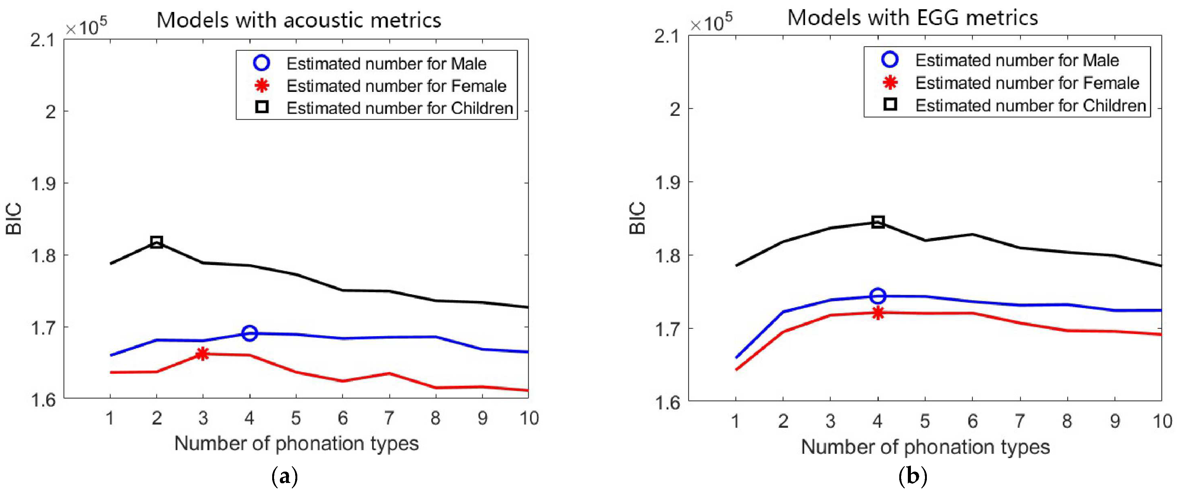
3.1. The Optimal Number of Clusters
3.2. Description of the Classification Voice Maps
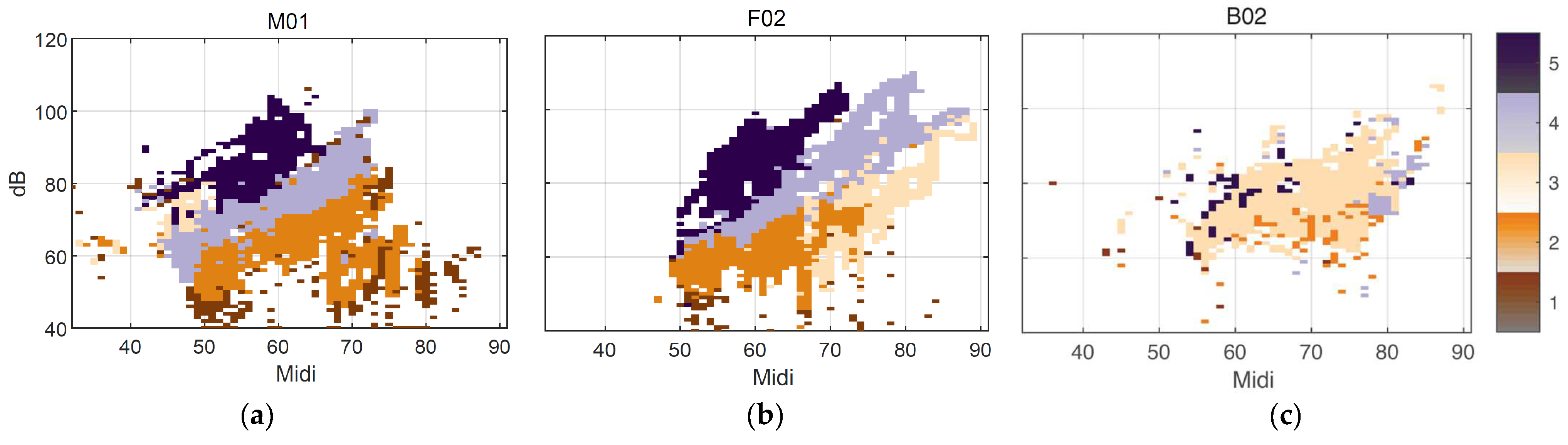
3.2.1. Intra-Participant Distribution
3.2.2. Union Maps of the Classification
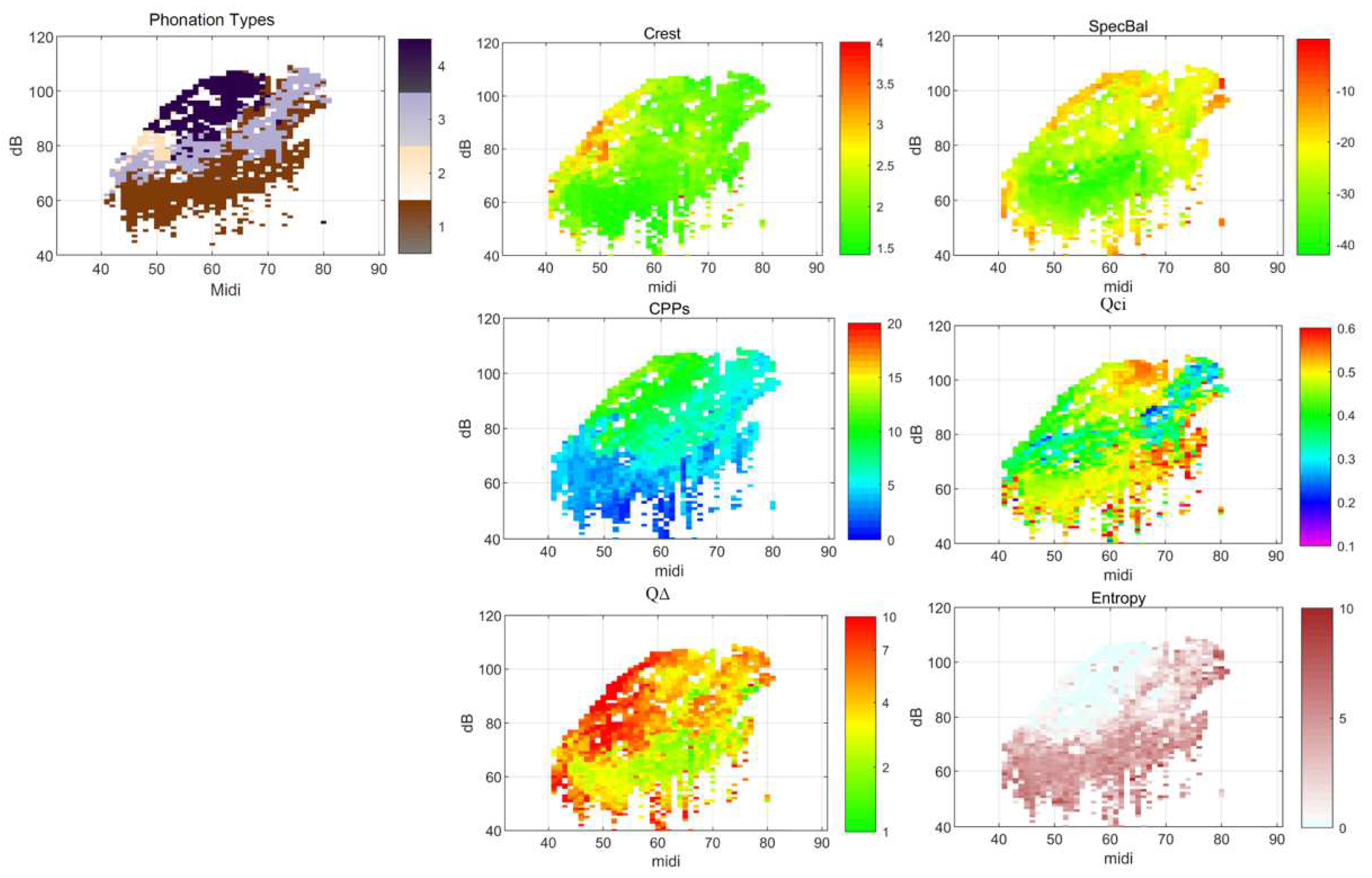
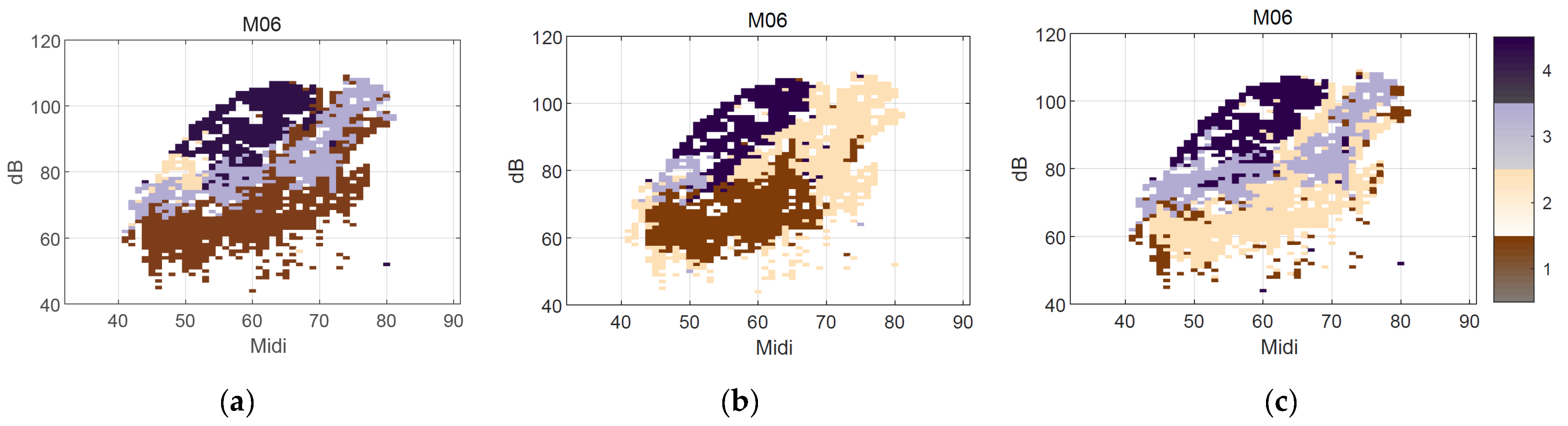
3.2.3. Acoustic Versus EGG Metrics
4. Discussion
5. Conclusions
Supplementary Materials
Author Contributions
Funding
Institutional Review Board Statement
Informed Consent Statement
Data Availability Statement
Acknowledgments
Conflicts of Interest
Appendix A

| Cluster Number | Phonation Type Map | Centroid Polar Plot (Range 0…1) | Metric Name | Single Metric Voice Map |
|---|---|---|---|---|
| k = 2 | 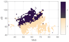 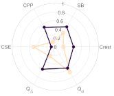 | Crest factor | 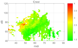 | |
| k = 3 |  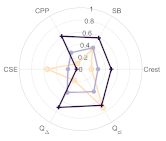 | Spectrum Balance | 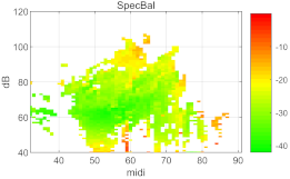 | |
| k = 4 | 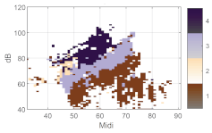 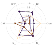 | CPPs | 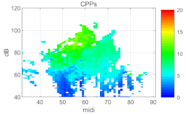 | |
| k = 5 | 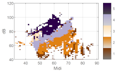  | Qci | 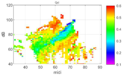 | |
| k = 6 |  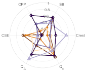 | Q∆ | 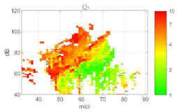 | |
| Speech range profile |  | CSE |  | |
| Cluster Number | Phonation Type Map | Centroid Polar Plot (Range 0…1) | Metric Name | Single Metric Voice Map |
|---|---|---|---|---|
| k = 2 |   | Crest factor |  | |
| k = 3 |  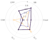 | Spectrum Balance |  | |
| k = 4 | 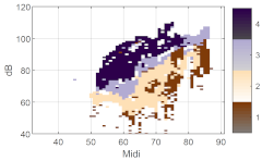  | CPPs | 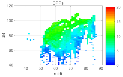 | |
| k = 5 | 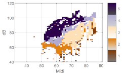 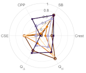 | Qci | 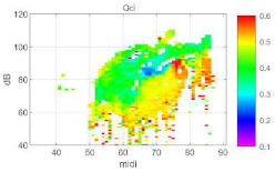 | |
| k = 6 | 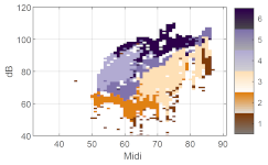 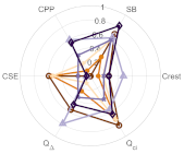 | Q∆ | 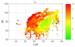 | |
| Speech range profile |  | CSE | 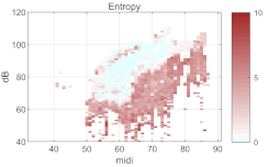 | |
| Cluster Number | Phonation Type Maps | Centroid Polar Plot (Range 0…1) | Metric Name | Single Metric Voice Map |
|---|---|---|---|---|
| k = 2 | 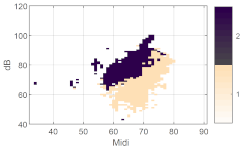 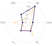 | Crest factor | 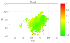 | |
| k = 3 |  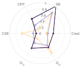 | Spectrum Balance | 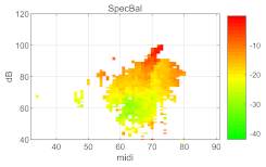 | |
| k = 4 |  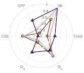 | CPPs | 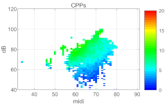 | |
| k = 5 | 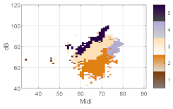 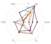 | Qci | 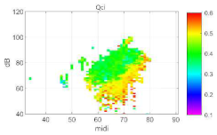 | |
| k = 6 |   | Q∆ | 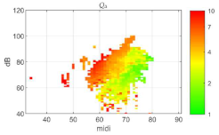 | |
| Speech range profile |  | CSE |  | |
| k | Centroid | Group | Crest Factor (dB) | SB (dB) | CPP (dB) | CSE | Q | Qci | Inferred Phonation Type |
|---|---|---|---|---|---|---|---|---|---|
| 2 | 1 | Male | 1.829 | −31.716 | 5.410 | 3.709 | 1.707 | 0.468 | soft |
| Female | 1.789 | −26.473 | 5.114 | 4.328 | 1.533 | 0.489 | soft | ||
| Children | 1.953 | −18.478 | 4.932 | 4.514 | 2.885 | 0.482 | soft | ||
| 2 | Male | 2.310 | −24.547 | 9.762 | 0.387 | 3.702 | 0.424 | loud | |
| Female | 2.083 | −19.495 | 8.659 | 0.579 | 3.636 | 0.403 | loud | ||
| Children | 2.329 | −12.529 | 8.436 | 1.231 | 5.260 | 0.395 | loud | ||
| 3 | 1 | Male | 1.820 | −31.693 | 5.269 | 4.294 | 1.449 | 0.493 | soft |
| Female | 1.799 | −26.559 | 5.062 | 4.442 | 1.470 | 0.497 | soft | ||
| Children | 1.955 | −18.389 | 4.796 | 4.733 | 2.792 | 0.493 | soft | ||
| 2 | Male | 2.003 | −27.684 | 7.291 | 0.957 | 3.125 | 0.370 | transition | |
| Female | 1.843 | −21.998 | 6.958 | 1.154 | 3.199 | 0.360 | transition | ||
| Children | 2.064 | −17.004 | 6.847 | 1.810 | 4.275 | 0.382 | transition | ||
| 3 | Male | 2.532 | −22.843 | 11.490 | 0.154 | 4.130 | 0.475 | loud | |
| Female | 2.283 | −17.535 | 10.083 | 0.216 | 4.003 | 0.443 | loud | ||
| Children | 2.530 | −9.117 | 9.588 | 1.036 | 6.052 | 0.414 | loud | ||
| 4 | 1 | Male | 1.820 | −31.700 | 5.267 | 4.296 | 1.444 | 0.493 | soft |
| Female | 1.798 | −26.608 | 5.057 | 4.446 | 1.467 | 0.497 | soft | ||
| Children | 1.891 | −22.639 | 4.302 | 4.759 | 3.112 | 0.490 | soft | ||
| 2 | Male | 2.975 | −26.402 | 10.936 | 0.215 | 4.167 | 0.428 | low modal | |
| Female | 2.487 | −21.014 | 10.494 | 0.158 | 4.124 | 0.425 | low modal | ||
| Children | 2.077 | −17.439 | 6.856 | 1.688 | 4.435 | 0.378 | low modal | ||
| 3 | Male | 1.973 | −27.858 | 7.230 | 0.994 | 3.112 | 0.366 | transition | |
| Female | 1.837 | −22.417 | 6.940 | 1.169 | 3.201 | 0.356 | transition | ||
| Children | 2.111 | −10.015 | 5.991 | 4.385 | 2.450 | 0.487 | transition | ||
| 4 | Male | 2.224 | −20.864 | 11.427 | 0.164 | 3.994 | 0.499 | loud | |
| Female | 2.063 | −14.266 | 9.378 | 0.368 | 3.785 | 0.459 | loud | ||
| Children | 2.519 | −9.527 | 9.786 | 0.829 | 6.296 | 0.410 | loud | ||
| 5 | 1 | Male | 2.01 | −22.74 | 3.42 | 4.74 | 4.36 | 0.50 | soft |
| Female | 2.22 | −18.41 | 3.29 | 4.30 | 5.84 | 0.53 | soft | ||
| Children | 3.068 | −13.786 | 4.448 | 4.381 | 6.722 | 0.482 | soft | ||
| 2 | Male | 1.80 | −33.64 | 4.74 | 4.09 | 2.42 | 0.48 | transition | |
| Female | 1.70 | −31.61 | 3.90 | 4.40 | 3.43 | 0.49 | transition | ||
| Children | 1.873 | −22.840 | 4.283 | 4.758 | 3.037 | 0.488 | transition | ||
| 3 | Male | 3.30 | −28.58 | 7.41 | 1.48 | 8.67 | 0.42 | low modal | |
| Female | 1.87 | −23.19 | 5.46 | 4.30 | 2.02 | 0.49 | low modal | ||
| Children | 2.060 | −17.634 | 6.887 | 1.629 | 4.370 | 0.377 | low modal | ||
| 4 | Male | 2.04 | −28.88 | 6.94 | 1.53 | 4.69 | 0.37 | falsetto | |
| Female | 1.91 | −22.52 | 7.15 | 1.38 | 4.15 | 0.36 | falsetto | ||
| Children | 1.995 | −10.352 | 6.221 | 4.311 | 2.293 | 0.484 | falsetto | ||
| 5 | Male | 2.44 | −21.87 | 11.27 | 0.27 | 6.87 | 0.48 | loud | |
| Female | 2.35 | −18.48 | 10.17 | 0.35 | 6.62 | 0.44 | loud | ||
| Children | 2.427 | −9.160 | 10.077 | 0.642 | 6.033 | 0.406 | loud | ||
| 6 | 1 | Male | 2.020 | −24.113 | 7.870 | 0.811 | 3.446 | 0.309 | soft |
| Female | 1.708 | −31.765 | 4.632 | 4.123 | 1.390 | 0.497 | soft | ||
| Children | 2.092 | −17.451 | 3.604 | 4.943 | 5.341 | 0.535 | soft | ||
| 2 | Male | 1.814 | −32.139 | 5.199 | 4.536 | 1.350 | 0.497 | transition | |
| Female | 1.890 | −21.419 | 5.467 | 4.761 | 1.553 | 0.496 | transition | ||
| Children | 3.352 | −13.193 | 4.898 | 4.073 | 6.815 | 0.447 | transition | ||
| 3 | Male | 1.909 | −22.562 | 7.087 | 1.206 | 2.655 | 0.439 | low modal | |
| Female | 2.510 | −21.150 | 10.551 | 0.151 | 4.137 | 0.427 | low modal | ||
| Children | 1.849 | −23.378 | 4.573 | 4.660 | 2.640 | 0.478 | low modal | ||
| 4 | Male | 2.990 | −26.321 | 10.941 | 0.207 | 4.183 | 0.428 | high modal | |
| Female | 1.755 | −25.489 | 6.862 | 1.103 | 3.073 | 0.390 | high modal | ||
| Children | 2.064 | −17.656 | 6.906 | 1.613 | 4.388 | 0.376 | high modal | ||
| 5 | Male | 2.000 | −35.203 | 6.699 | 1.251 | 3.093 | 0.388 | falsetto | |
| Female | 1.964 | −18.399 | 7.246 | 1.102 | 3.414 | 0.322 | falsetto | ||
| Children | 2.009 | −9.954 | 6.366 | 4.241 | 2.239 | 0.477 | falsetto | ||
| 6 | Male | 2.261 | −21.097 | 11.878 | 0.110 | 4.128 | 0.503 | loud | |
| Female | 2.076 | −14.320 | 9.609 | 0.282 | 3.867 | 0.463 | loud | ||
| Children | 2.424 | −9.169 | 10.097 | 0.625 | 6.039 | 0.406 | loud |
References
- Kuang, J.; Keating, P. Vocal fold vibratory patterns in tense versus lax phonation contrasts. J. Acoust. Soc. Am. 2014, 136, 2784–2797. [Google Scholar] [CrossRef] [PubMed] [Green Version]
- Yu, K.; Lam, H. The role of creaky voice in Cantonese tone perception. J. Acoust. Soc. Am. 2014, 136, 1320–1333. [Google Scholar] [CrossRef] [PubMed] [Green Version]
- Wang, C.; Tang, C. The Falsetto Tones of the Dialects in Hubei Province. In Proceedings of the 6th International Conference on Speech Prosody, SP 2012, Shanghai, China, 22–25 May 2012; Volume 1. [Google Scholar]
- Davidson, L. The versatility of creaky phonation: Segmental, prosodic, and sociolinguistic uses in the world’s languages. Wiley Interdiscip. Rev. Cogn. Sci. 2021, 12, e1547. [Google Scholar] [CrossRef] [PubMed]
- Gordon, M.; Ladefoged, P. Phonation types: A cross-linguistic overview. J. Phon. 2001, 29, 383–406. [Google Scholar] [CrossRef] [Green Version]
- Sundberg, J. Vocal fold vibration patterns and modes of phonation. Folia Phoniatr. Logop. 1995, 47, 218–228. [Google Scholar] [CrossRef]
- Borsky, M.; Mehta, D.D.; Van Stan, J.H.; Gudnason, J. Modal and non-modal voice quality classification using acoustic and electroglottographic features. IEEE/ACM Trans. Audio Speech Lang. Process. 2017, 25, 2281–2291. [Google Scholar] [CrossRef]
- Hillenbrand, J.; Cleveland, R.A.; Erickson, R.L. Acoustic correlates of breathy vocal quality. J. Speech Hear. Res. 1994, 37, 769–778. [Google Scholar] [CrossRef] [PubMed]
- Gowda, D.; Kurimo, M. Analysis of breathy, modal and pressed phonation based on low frequency spectral density. In Proceedings of the Interspeech, Lyon, France, 25–19 August 2013; pp. 3206–3210. [Google Scholar] [CrossRef]
- Kadiri, S.R.; Alku, P. Glottal features for classification of phonation type from speech and neck surface accelerometer signals. Comput. Speech Lang. 2021, 70, 101232. [Google Scholar] [CrossRef]
- Hsu, T.Y.; Ryherd, E.E.; Ackerman, J.; Persson Waye, K. Psychoacoustic measures and their relationship to patient physiology in an intensive care unit. J. Acoust. Soc. Am. 2011, 129, 2635. [Google Scholar] [CrossRef]
- Kadiri, S.R.; Alku, P.; Yegnanarayana, B. Analysis and classification of phonation types in speech and singing voice. Speech Commun. 2020, 118, 33–47. [Google Scholar] [CrossRef]
- Selamtzis, A.; Ternstrom, S. Analysis of vibratory states in phonation using spectral features of the electroglottographic signal. J. Acoust. Soc. Am. 2014, 136, 2773–2783. [Google Scholar] [CrossRef] [PubMed]
- Ternström, S.; Pabon, P. Voice Maps as a Tool for Understanding and Dealing with Variability in the Voice. Appl. Sci. 2022, 12, 11353. [Google Scholar] [CrossRef]
- Selamtzis, A.; Ternström, S. Investigation of the relationship between electroglottogram waveform, fundamental frequency, and sound pressure level using clustering. J. Voice 2017, 31, 393–400. [Google Scholar] [CrossRef] [PubMed]
- Ternstrom, S. Normalized time-domain parameters for electroglottographic waveforms. J. Acoust. Soc. Am. 2019, 146, EL65. [Google Scholar] [CrossRef] [Green Version]
- Johansson, D. Real-Time Analysis, in SuperCollider, of Spectral Features of Electroglottographic Signals. Master’s Thesis, KTH Royal Institute of Technology, Stockholm, Sweden, 2016. Available online: https://kth.diva-portal.org/smash/get/diva2:945805/FULLTEXT01.pdf (accessed on 24 November 2022).
- Pabon, J.P.H. Objective acoustic voice-quality parameters in the computer phonetogram. J. Voice 1991, 5, 203–216. [Google Scholar] [CrossRef]
- Fant, G. The LF-model revisited. Transformations and frequency domain analysis. Speech Trans. Lab. Q. Rep. Royal Inst. Tech. Stockholm 1995, 36, 119–156. [Google Scholar]
- Awan, S.N.; Solomon, N.P.; Helou, L.B.; Stojadinovic, A. Spectral-cepstral estimation of dysphonia severity: External validation. Ann. Otol. Rhinol. Laryngol. 2013, 122, 40–48. [Google Scholar] [CrossRef]
- Ternström, S.; Bohman, M.; Södersten, M. Loud speech over noise: Some spectral attributes, with gender differences. J. Acoust. Soc. Am. 2006, 119, 1648–1665. [Google Scholar] [CrossRef]
- Patel, R.R.; Ternstrom, S. Quantitative and Qualitative Electroglottographic Wave Shape Differences in Children and Adults Using Voice Map-Based Analysis. J. Speech Lang. Hear. Res. 2021, 64, 2977–2995. [Google Scholar] [CrossRef]
- Ternström, S.; Johansson, D.; Selamtzis, A. FonaDyn—A system for real-time analysis of the electroglottogram, over the voice range. SoftwareX 2018, 7, 74–80. [Google Scholar] [CrossRef]
- Damsté, P.H. The phonetogram. Pract. Otorhinolaryngol. 1970, 32, 185–187. [Google Scholar]
- Schutte, H.K.; Seidner, W. Recommendation by the Union of European Phoniatricians (UEP): Standardizing voice area measurement/phonetography. Folia. Phoniatr. 1983, 35, 286–288. [Google Scholar] [CrossRef] [PubMed]
- Pabon, P. Mapping Individual Voice Quality over the Voice Range: The Measurement Paradigm of the Voice Range Profile. Comprehensive Summary. Ph.D. Thesis, KTH Royal Institute of Technology, Stockholm, Sweden, 2018. [Google Scholar]
- Arthur, D.; Vassilvitskii, S. k-means++: The advantages of careful seeding. In Proceedings of the Eighteenth Annual ACM-SIAM Symposium on Discrete Algorithms, New Orleans, LA, USA, 7–9 January 2007; pp. 1027–1035. [Google Scholar]
- Childers, D.G.; Lee, C.K. Vocal quality factors: Analysis, synthesis, and perception. J. Acoust. Soc. Am. 1991, 90, 2394–2410. [Google Scholar] [CrossRef] [PubMed] [Green Version]
- Pabon, P.; Ternstrom, S. Feature Maps of the Acoustic Spectrum of the Voice. J. Voice 2020, 34, 161.e1–161.e26. [Google Scholar] [CrossRef] [PubMed] [Green Version]
- Stomeo, F.; Rispoli, V.; Sensi, M.; Pastore, A.; Malagutti, N.; Pelucchi, S. Subtotal arytenoidectomy for the treatment of laryngeal stridor in multiple system atrophy: Phonatory and swallowing results. Braz. J. Otorhinolaryngol. 2016, 82, 116–120. [Google Scholar] [CrossRef] [PubMed]
- Kuang, J. Covariation between voice quality and pitch: Revisiting the case of Mandarin creaky voice. J. Acoust. Soc. Am. 2017, 142, 1693. [Google Scholar] [CrossRef] [PubMed]
- Ladefoged, P. Cross-Linguistic Studies of Speech Production. In The Production of Speech; MacNeilage, P.F., Ed.; Springer: New York, NY, USA, 1983; pp. 177–188. [Google Scholar]
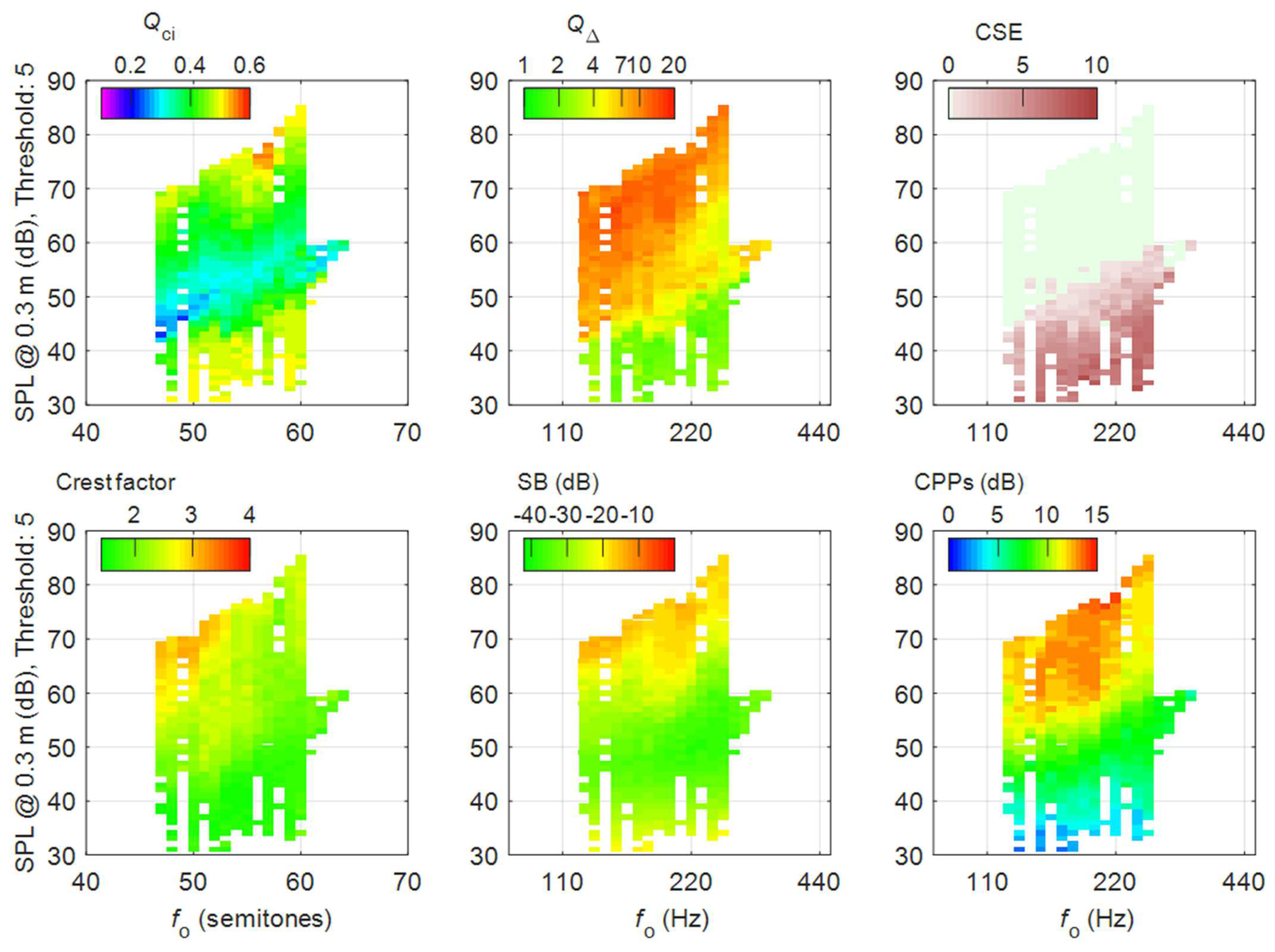


| Symbol | Definition | Range | |
|---|---|---|---|
| EGG Metrics | Qci | quotient of contact by integration | 0…1 |
| Q∆ | normalized peak derivative | 1…10 | |
| CSE | cycle-rate sample entropy | 0…10 | |
| Acoustic Metrics | crest factor | ratio of the peak amplitude of the RMS amplitude | 3…12 dB |
| SB | spectrum balance | −40…0 dB | |
| CPPs | cepstral peak prominence smoothed | 0…15 dB | |
| Male M01 | Female F06 | Child B09 | |
|---|---|---|---|
| k = 2 |  |  | 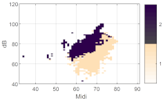 |
| k = 3 |  | 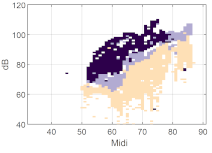 |  |
| k = 4 |  | 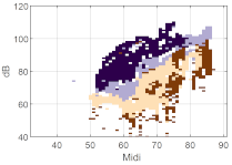 | 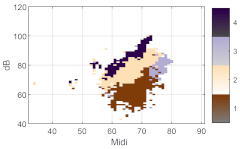 |
| k = 5 |  |  |  |
| k = 6 |  |  |  |
| Speech range profile | 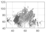 |  | 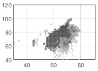 |
| 13 Males | 13 Females | 22 Children | |
|---|---|---|---|
| k = 2 | 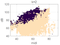 | 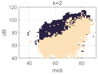 | 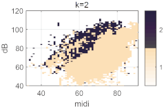 |
| k = 3 | 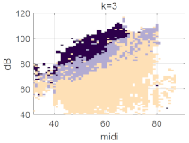 | 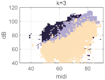 | 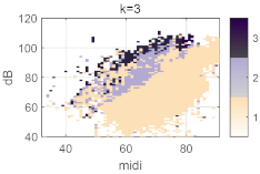 |
| k = 4 | 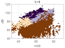 | 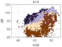 | 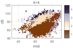 |
| k = 5 | 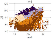 | 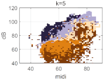 | 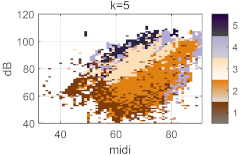 |
| k = 6 | 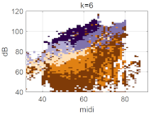 | 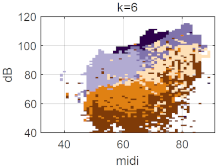 |  |
Publisher’s Note: MDPI stays neutral with regard to jurisdictional claims in published maps and institutional affiliations. |
© 2022 by the authors. Licensee MDPI, Basel, Switzerland. This article is an open access article distributed under the terms and conditions of the Creative Commons Attribution (CC BY) license (https://creativecommons.org/licenses/by/4.0/).
Share and Cite
Cai, H.; Ternström, S. Mapping Phonation Types by Clustering of Multiple Metrics. Appl. Sci. 2022, 12, 12092. https://doi.org/10.3390/app122312092
Cai H, Ternström S. Mapping Phonation Types by Clustering of Multiple Metrics. Applied Sciences. 2022; 12(23):12092. https://doi.org/10.3390/app122312092
Chicago/Turabian StyleCai, Huanchen, and Sten Ternström. 2022. "Mapping Phonation Types by Clustering of Multiple Metrics" Applied Sciences 12, no. 23: 12092. https://doi.org/10.3390/app122312092