Autonomous Navigation Based on the Earth-Shadow Observation near the Sun–Earth L2 Point

Abstract

This paper is devoted to a novel autonomous navigation method for spacecraft around the Sun–Earth L2 point. In contrast to the previous navigation methods, which rely on ground-based or inter-spacecraft measurements, the proposed method determines the orbit based on Earth-shadow measurements. First, the navigation framework using the Earth-shadow measurement is proposed. Second, the geometric analysis is used to derive the mathematical model of the Earth-shadow measurements. Then, the fifth-degree Cubature Kalman filter (CKF) is designed to estimate the states of the spacecraft. Numerical simulations are implemented to validate the performance of the proposed navigation method. Finally, the simulation results show that the navigation system is observable and that the proposed method could be potentially useful for an autonomous navigation mission near the Sun–Earth L2 point in the future.

1. Introduction

Recently, usage of the periodic orbits around the Lagrange points has attracted great attention, and many missions have been carried out or planned, such as the Chang’e-4 and the Deep Space Gateway [1,2]. One of the important issues in these missions is to accurately determine the orbit of the spacecraft. The knowledge of the spacecraft state is essential for substantial guidance and control, and can be potentially useful for some scientific purposes, such as gravitational wave detection and gravitational field recovery [3,4]. Thus, it is necessary to investigate the navigation problem of the spacecraft in three-body dynamics.

The typical space mission, ISEE-3, runs around the Sun–Earth L1 point with the Halo orbit. The precision of this navigation method is about 4 to 8 km during the two circles’ orbit calculation [5]. The navigation accuracy of CE-2 depending on the unified S-band measurement and very long baseline interferometry measurement can reach 2 km by using overlap analysis [6]. The typical accuracies of orbit determination methods are on the order of several hundred meters in position and several mm/s in velocity with 5–7 days tracking data. The European Space Agency (ESA) ground stations are designed and built to comply with the carrier stability requirements as defined in the ECSS-E-50-02A Ranging and Doppler tracking standard, which shows that the measurement precision of the Doppler tracking is in the magnitude of 0.1 mm/s, whilst for distance it is 1 m. The Radioscience Bepi-Colombo MORE experiment used Ka band radio links to make accurate measurements of the spacecraft range and range rate. Tropospheric zenith wet delays range from 1.5 cm to 10 cm, and the high variability impairs the accuracy of these measurements [7,8]. The combination of very long baseline interferometry data with range or Doppler data can improve the orbit accuracy in the L2 region compared with the range or Doppler data only. The technique and analysis method used can provide the foundation for future Earth–Moon libration point spacecraft missions, including the CE-4 relay satellite in the L2 region [9].

Nowadays, collinear Lagrange points of the restricted three-body problem are receiving increasing attention because of their special dynamical properties and unique geometrical positions [10,11,12]. There are five Lagrange points in the Sun–Earth three-body system. This study focuses on navigation around the Lagrange point L2. Because orbital motion near the Lagrange point L2 is extremely sensitive to the initial value, the small error will be quickly amplified. The spacecraft needs to conduct orbital maneuvers frequently, otherwise, it will deviate from the target area soon. Therefore, the navigation needs to meet high-precision requirements [13,14,15]. Vasile et al. [16] proposed an autonomous navigation method for deep space spacecraft, designed for measuring the attitude and azimuth of celestial bodies. This method is to determine the spacecraft state using the optical measurement data processed with the least-square-degree Kalman filter algorithm.

Focusing on the spacecraft navigation technology, Yim et al. [17] conducted a study about the observability of relative navigation in two-body dynamics by line-of-sight measurement under the influence of J2 perturbation. The results show that the performance of the navigation system can be improved by selecting the orbital parameters properly. Chen et al. [18] investigated the navigation method using space-based angle measurement data. This method calculates the orbital parameters by the Direct Method or Newton method based on the initial value and proves that the spacecraft orbit can be determined by the space-based angle measurement data. Zhang et al. [19] considered the relative motion and estimated the parameters of noncooperative targets from the perspective of the nonlinearly constrained optimization problem. The author also proposed a monocular vision method and verified its effectiveness through numerical simulation. Liu [20] took the space-based monitoring system as the research background and analyzed the space-based detectability of noncooperative targets. The author also improved the filtering algorithms and key technologies for initial navigation and combined navigation of space-based noncooperative targets, which are based on the angle measurement information. Lu [21] discussed the autonomous optical navigation technology of the deep space spacecraft, designed the image processing algorithm and information extraction algorithm, and analyzed the observability of the system by the numerical analysis method. The method of determining the relative orbit of two spacecraft by measuring their relative distance is commonly used. Although a great deal of the distance measurement method was put forward earlier, it is difficult to achieve high-precision requirements in a complex space environment. Moreover, while the relative navigation between the objective spacecraft and the observation spacecraft can be achieved by the other measurement information, the absolute navigation is hard to achieve [22,23,24].

Chen et al. [25] proposed an autonomous navigation method for spacecraft based on intersatellite ranging and orbit orientation parameter constraints. This method assumes that the coordinates connected to the Earth and the absolute orientation of the constellation in inertial space cannot be established solely through inter-satellite ranging. Thus, its orbit must be determined by combining dynamic equations and prediction information [26,27,28]. Tang [29] studied the inter-satellite distance measurement technology in the static and dynamic environment, discussed the autonomous navigation technology based on the intersatellite distance measurement, and proposed a ranging technology that can gradually improve the precision in a static environment. The study also proved that the high-precision distance between spacecraft could not be obtained only through inter-satellite distance measurement [30,31,32].

Based on the related Earth-shadow researches [33,34], we focus on the autonomous navigation at the Sun–Earth L2 point. The difficulty of navigation around the Sun–Earth L2 point is that there are few observations available for navigation [35,36,37]. This paper studies the autonomous navigation method based on the Earth-shadow observation near the Sun–Earth L2 point. This method determines the position and velocity of the spacecraft by measuring the proportion that the Sun is blocked by the Earth. In Section 2, we build the dynamic model and establish the measurement model of the Earth-shadow. Then, we derive the expression of the measurement function from three different observation scenarios. In Section 3, we apply the fifth-degree cubature Kalman filter algorithm to simulate the different models with an amplitude of 5000 km along the X direction. In Section 4, we obtain the simulation results of navigation and provide the analysis of the simulation results. Finally, the conclusions are given in Section 5.

2. Design of Navigation System

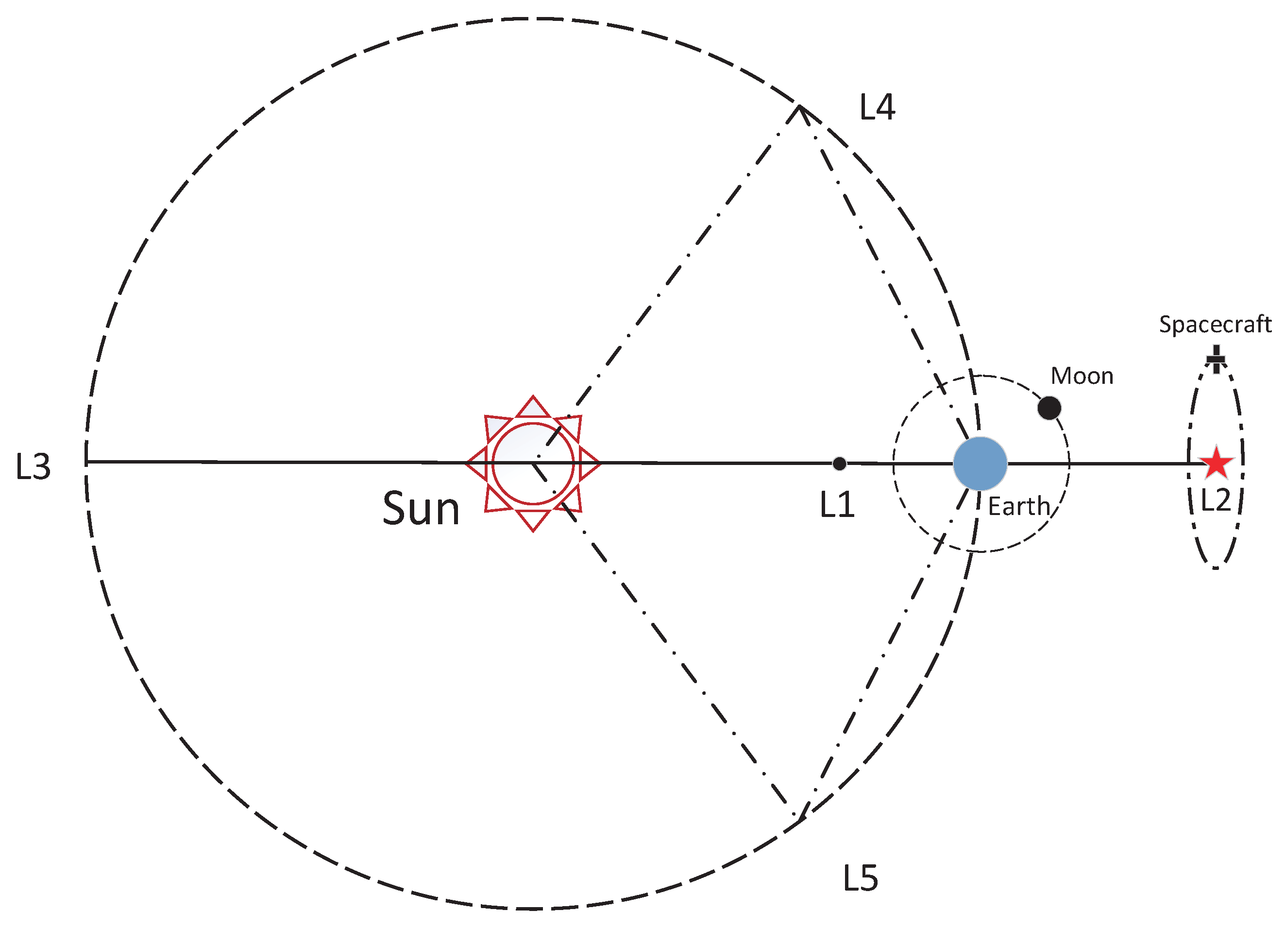
2.1. Circular Restricted Three-Body Problem

The Circular Restricted Three-body Problem (CRTBP) is discussed in this paper to describe the motion of spacecraft in the Sun–Earth system. As shown in Figure 1, the CRTBP model reflects the motion of the spacecraft. The spacecraft is subjected to the gravitational force of the two primary bodies, which move in circular orbits around their barycenter point. It is assumed that the masses of the primary celestial bodies $P_1$ and $P_2$ are $M_1$ and $M_2$, respectively. The mass of the spacecraft m is much smaller than $M_1$ and $M_2$. Thus, it cannot practically influence the motion of the primaries or change the position of their barycenter.

The motion of the spacecraft is described in the rotating frame. The origin center is at the barycenter, with the x-axis pointed in the direction from $P_1$ towards $P_2$. The z-axis is aligned with the direction of the angular momentum vector. The y-axis satisfies the right-handed rule.

Typically, in order to simplify the calculation, the CRTBP dynamics are studied in the nondimensional form. The distance between the two primary bodies is denoted by L. Meanwhile, the constant angular velocity of the two primary bodies around the barycenter is denoted by $\omega$. The characteristic mass $\left[M\right]$, the characteristic length $\left[L\right]$, and the characteristic time $\left[T\right]$ are nondimensional variables, which are defined as

$$\begin{array}{c}\left\{\begin{array}{c}\left[M\right]=M_1+M_2\hfill \\ \left[L\right]=∥P_1{P}_2∥\hfill \\ \left[T\right]={\left[\frac{{∥P_1{P}_2∥}^3}{G\left(M_1+M_2\right)}\right]}^{\frac{1}{2}}.\hfill \end{array}\right.\end{array}$$

(1)

The characteristic mass parameter $\mu$ is defined as

$$\begin{array}{c}\mu =\frac{M_2}{M_1+M_2}.\end{array}$$

(2)

In the CRTBP, the nondimensional dynamic model in the rotating frame is expressed as follows:

$$\ddot{\mathit{r}}+2\left[\begin{array}{c}-\dot{y}\\ \dot{x}\\ 0\end{array}\right]={\left[\frac{\partial \Omega }{\partial \mathit{r}}\right]}^{\mathrm{T}},$$

(3)

where $\Omega$ is the equivalent potential energy function

$$\left\{\begin{array}{c}\Omega =\frac{1}{2}\left(x^2+y^2\right)+\frac{1-\mu }{r_1}+\frac{\mu }{r_2}\hfill \\ r_1=\sqrt{{(x+\mu )}^2+y^2+z^2}\hfill \\ r_2=\sqrt{{(x-1+\mu )}^2+y^2+z^2}.\hfill \end{array}\right.$$

(4)

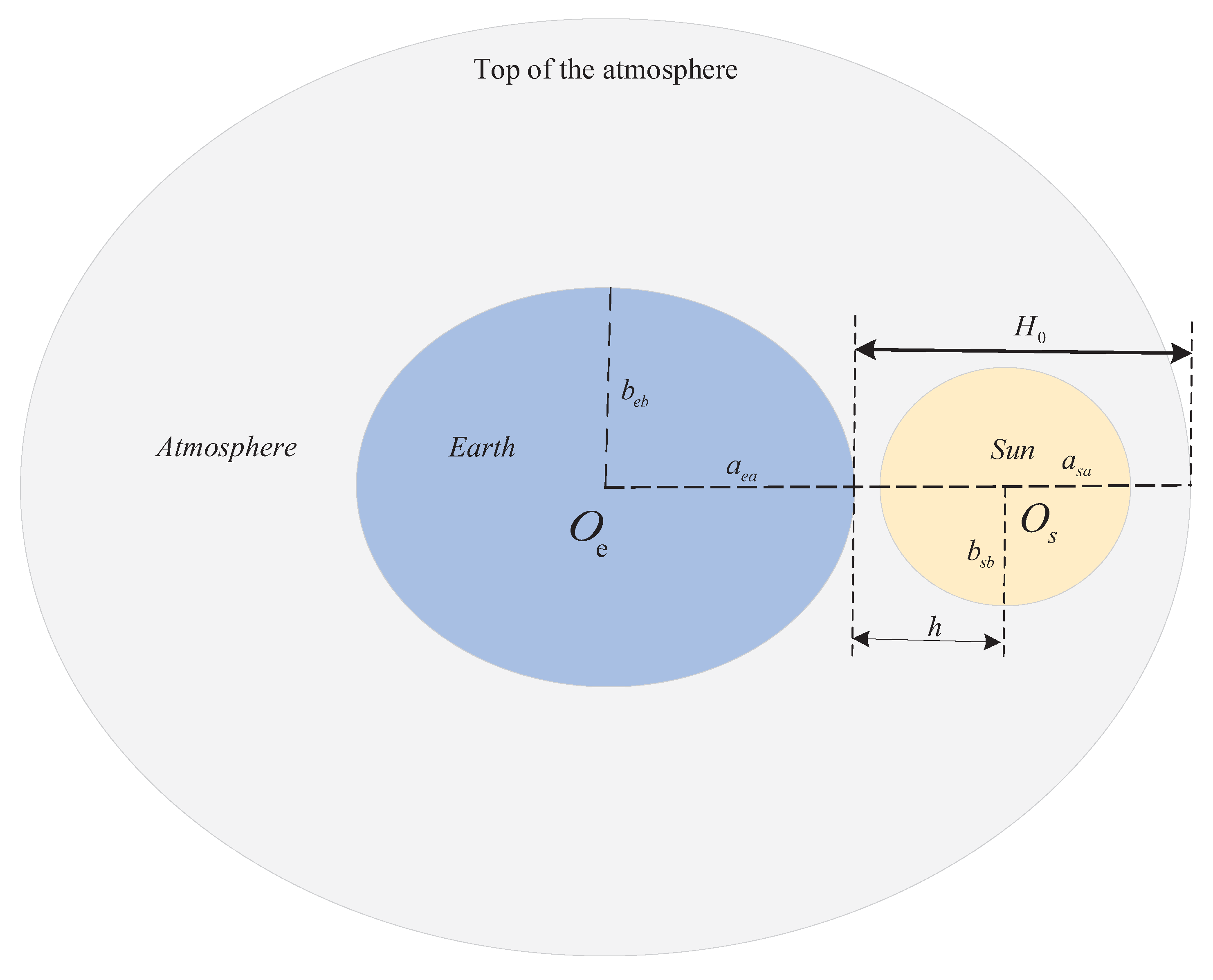
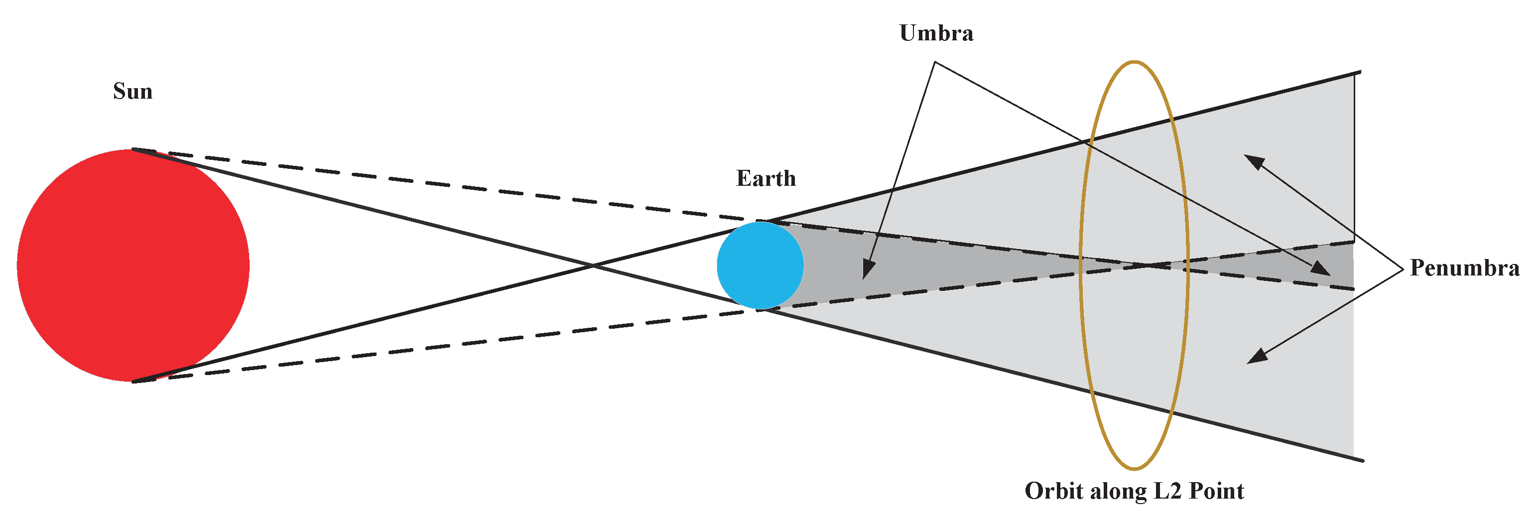
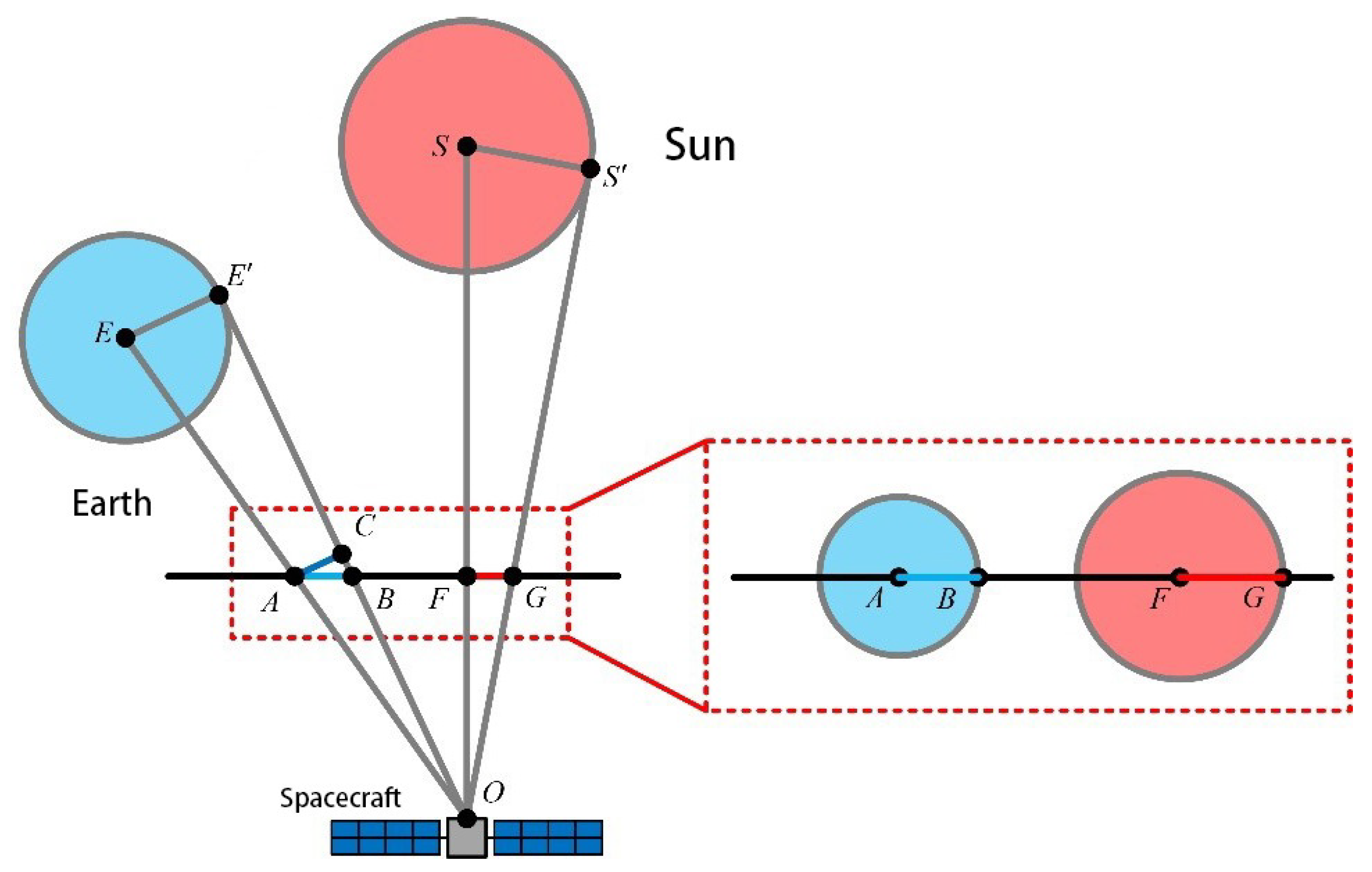
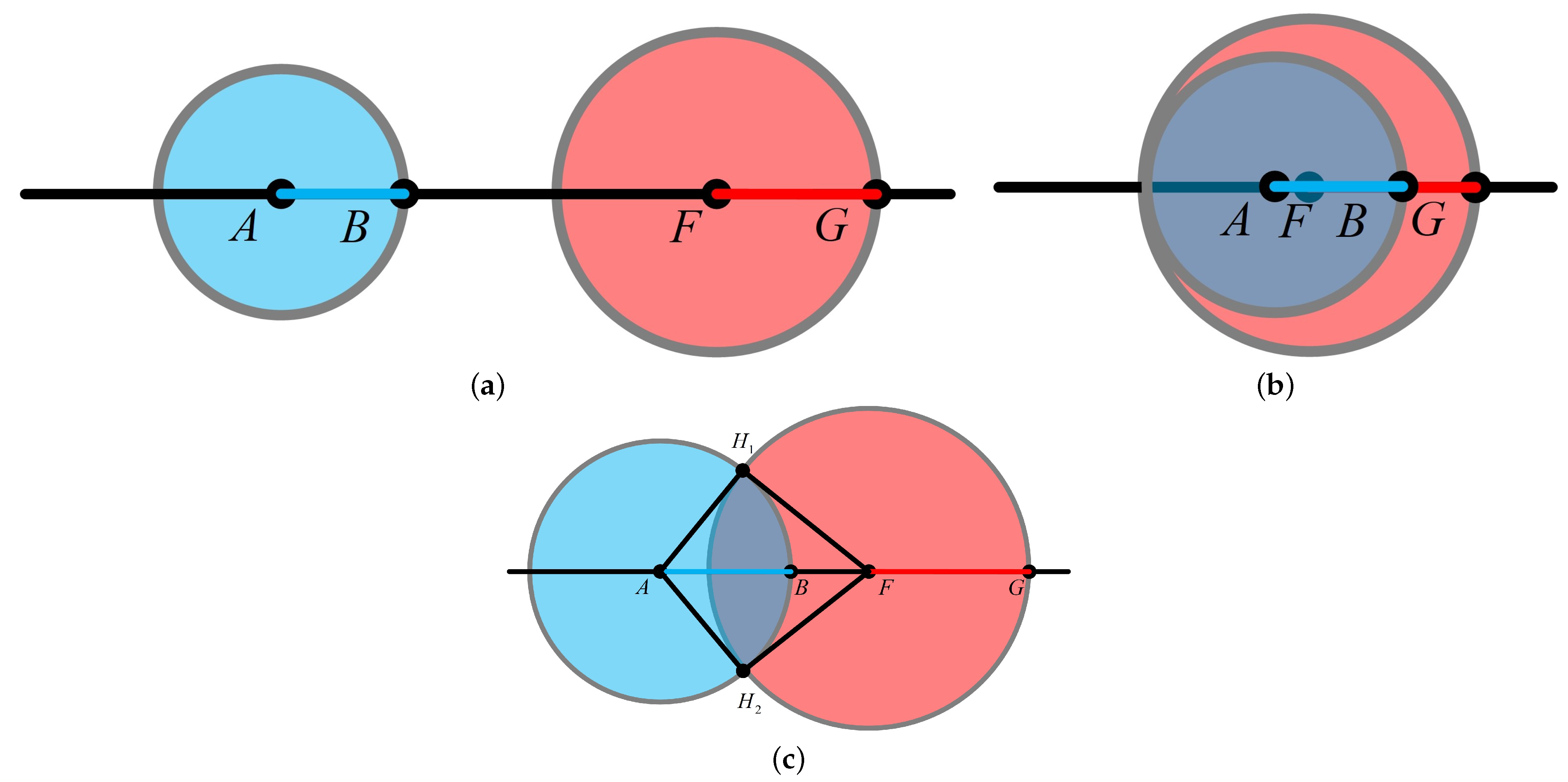
2.2. The Earth-Shadow Measurement Model

Firstly, we introduce the Sun–Earth L2 point. The Sun–Earth Lagrange point refers to the space balance point between the Sun and the Earth. There are 5 points in total, as shown in Figure 2. The important points are L1 and L2 for humans to explore and utilize space resources in the future, which are located on both sides and 1.5 million kilometers away from the Earth. Since the point L1 is located between the Sun and the Earth, it is of great significance to detect the environment of the Sun and the Earth. Point L2 is located on the other side of the Earth, which faces away from the Sun. Typically, Halo orbits in the vicinity of the Sun–Earth Lagrange points, such as L1 or L2, are regarded as suitable locations for astronomical observation because the spacecraft around these places are able to maintain the same orientation and consume little fuel for station keeping. Halo orbit missions such as ISEE-3, WMAP, Herschel, and Chang’e-2 are notable successful projects [38,39]. Because of numerous advantages such as facing away from the Sun, stable lighting conditions and the reduced effect of visible light and infrared radiation, it is worthy exploring this more deeply in future deep space explorations.

In some special circumstances, the Sun is blocked by the Earth, forming the Earth-shadow area. This phenomenon is called Earth-shadow [40,41,42]. It is apparent that the Earth-shadow is closely related to the relative position of the Sun, the Earth, and the spacecraft.

In fact, the Sun is a ball of gases. The diameter of the Sun varies depending on the optical wavelength considered. It is assumed that the errors regarding the diameter of the Sun are ten kilometers. As shown in Figure 3, the Earth and the Sun on the projection plane are both ellipses, and $O_e$ and $O_s$ are the centers of them, respectively. It is assumed that the equivalent radius of the Sun is $a_{sa}$. The equivalent radius of the Earth is $a_{ea}$. Generally, astronomers define the boundary of the Sun with the wavelength of 500 nm. The theoretical radius of the Sun and the Earth are noted $b_{sb}$ and $b_{eb}$. The errors of the diameter of the Sun between different wavelengths are far smaller than the distance between the spacecraft and the Earth, the distance between the spacecraft and the Sun, and the diameters of the Earth and the Sun. Therefore, the error of the diameter of the Sun between different wavelengths can be considered as a small quantity. Moreover, the Sun also has a little flattening. The Earth itself is surrounded by atmosphere, which blurs the light and radiation transition between the surface of the earth and vacuum [43,44]. The function $f\left(h\right)$ that describes the radiation reduction coefficient is defined. This function computes the ratio between the solar radiation at the depth of h in the atmosphere and the radiation outside of the atmosphere. The thickness $H_0$ of the atmosphere on the image is different depending on the position of the satellite. For any point that has a distance h to the solid Earth in the direction from the center of the Earth $O_e$ to the center of the Sun $O_s$ on the image, $f\left(h\right)$ is given by

$$\begin{array}{c}f\left(h\right)=({\mu }_2-{\mu }_1)\frac{h}{H_0}+{\mu }_1,\end{array}$$

(5)

where ${\mu }_1$ is the radiation reduction coefficient at the boundary of the solid Earth and ${\mu }_2$ is the radiation reduction coefficient at the boundary of the atmosphere. Thus, ${\mu }_1=0$ and ${\mu }_2=1$.

In the situation that the Sun is totally blocked by the Earth, the overlapping ratio is defined as follows:

$$\begin{array}{c}rati{o}_{theory}=\frac{\pi b_{eb}^2}{\pi b_{sb}^2};rati{o}_{error}=\frac{\pi a_{ea}{b}_{eb}}{\pi a_{sa}{b}_{sb}}\end{array}$$

(6)

$$\begin{array}{c}{\Delta }_{overlap}=\frac{rati{o}_{theory}}{rati{o}_{error}}=\frac{\pi b_{eb}^2\pi a_{sa}{b}_{sb}}{\pi b_{sb}^2\pi a_{ea}{b}_{eb}},\end{array}$$

(7)

where $rati{o}_{theory}$ is the ratio of the overlapping area in theory condition, and $rati{o}_{error}$ is the ratio of the overlapping area while considering the atmosphere and oblateness of the Earth and the Sun in space. ${\Delta }_{overlap}$ is the observation model error between the theoretical and real space environment. From the above error analysis, we define the observation model errors ${\mathit{e}}_{obs}$ as follows:

$$\begin{array}{c}{\mathit{e}}_{obs}=f\left(h\right)+{\Delta }_{overlap}.\end{array}$$

(8)

As shown in Figure 4, the Earth-shadow area can be divided into the umbra shadow area and the penumbra shadow area. The umbra shadow is the area where the Sun is completely shielded by the Earth, and the penumbra shadow is the area where the Sun is partially shielded by the Earth. When the spacecraft passes through the penumbra shadow area, the proportion of the Sun being shielded by the Earth will change continuously, which provides the related information of the spacecraft orbit. The information is directly related to the light intensity of the current position and can be measured by the electric energy production of the solar panel or by optical sensors.

As shown in Figure 5, it is assumed that the spacecraft is located at the point O. The Earth and the Sun are located at point E and S. Points $E_1$ and $S_1$ are the tangent points of the two circles, respectively. OE and OS represent the distance from the spacecraft to the Earth and to the Sun, respectively. $E{E}^{\prime }$ and $S{S}^{\prime }$ represent the radius of the Earth and the Sun, respectively. $\angle EOS$ is the angle between the Earth, the spacecraft, and the Sun. It is apparent that the values of all the above parameters can be calculated through the ephemeris. The line AG is located in the plane composed of the Earth, the Sun, and the spacecraft and is one astronomical unit away from the spacecraft. In order to characterize the proportion of the Sun being shielded by the Earth, the Sun and the Earth are projected onto a plane, which is defined as the reference plane. The reference plane passes through the straight line AG and is perpendicular to the plane composed of the Earth, the Sun, and the spacecraft.

The distance between the spacecraft and the Earth and the distance between the spacecraft and the Sun are far longer than the scale of the spacecraft orbit around the Earth, and also longer than the radius of the Earth and the Sun. Therefore, it can be considered that $\angle EO{E}^{\prime }$ and $\angle SO{S}^{\prime }$ are very small, approximately equal to 0, such that the following relations are obtained:

$$\begin{array}{c}AO\approx BO\approx FO\approx GO\approx 1,\angle EOS=\angle AOF\approx \angle BOF.\end{array}$$

(9)

Perform auxiliary lines $AC\perp O{E}^{\prime }$. It can be deduced, from the geometric relationships, that

$$\begin{array}{c}\angle GOF=\angle SO{S}^{\prime },\angle OFG=\angle O{S}^{\prime }S,\angle O{E}^{\prime }E=\angle OCA\\ \angle OCA=\angle E^{\prime }OE,\angle ABC=\angle OBF,\angle ACB=\angle OFB.\end{array}$$

(10)

According to the principle of triangle similarity, $▵OS{S}^{\prime }\simeq ▵OGF,▵OE{E}^{\prime }\simeq ▵OAC,▵BAC\simeq ▵BOF$. Therefore,

$$\begin{array}{c}FG=S{S}^{\prime }\frac{OG}{OS}\approx \frac{S{S}^{\prime }}{OS}\\ AC=E{E}^{\prime }\frac{OA}{OE}\approx \frac{E{E}^{\prime }}{OE}\\ \angle CAB=\angle BOF.\end{array}$$

(11)

In the right triangle $▵ABC$ and $▵OGF$, AB and FG are given as

$$\begin{array}{c}AB=\frac{AC}{tan\angle CAB}=\frac{AC}{tan\angle BOF}\approx \frac{AC}{tan\angle EOS}\\ FG=FOtan\angle GOF=tan\angle GOF\approx 0,\end{array}$$

(12)

and the lines AB and FG represent the radius of the Earth and the Sun, respectively. Meanwhile, we can obtain the distance between the projection center of the Earth and the Sun, which is given as

$$AF\approx OFtan\angle AOF\approx tan\angle AOF.$$

(13)

As shown in Figure 6, according to the analysis of the spatial motion of the Sun, the Earth, and the spacecraft, it can be concluded that there are three different occlusion types in the whole cycle. The following sections will discuss the three different circumstances, respectively.

As shown in Figure 6a, when $AF\ge AB+FG$,

$$tan\angle AOF\ge tan\angle GOF+\frac{AC}{tan\angle EOS}\approx \frac{AC}{tan\angle EOS},$$

(14)

the Earth cannot block the Sun. Therefore, it can be obtained that the measurement function H is equal to zero.

As shown in Figure 6b, when $AF\le FG-AB$, the Earth’s projection is included in the Sun’s projection. Therefore, the measurement function H is given in the following formula:

$$H=\frac{\pi A{B}^2}{\pi G{F}^2}=\frac{A{B}^2}{G{F}^2}.$$

(15)

As shown in Figure 6c, when $FG-AB\le AF\le FG+AB$,

$$tan\angle GOF-\frac{AC}{tan\angle EOS}\le tan\angle AOF\le tan\angle GOF+\frac{AC}{tan\angle EOS},$$

(16)

and the Earth’s projection and the Sun’s projection have overlapping parts. Thus, the measurement function H is given as

$$H=\frac{S_{\mathrm{overlap}}}{\pi G{F}^2},$$

(17)

where $S_{overlap}$ represents the overlapping areas of the Earth’s projection and the Sun’s projection, which can be calculated by adding the area of Fan $A{H}_1{H}_2$ and Fan $F{H}_1{H}_2$, and by subtracting the area of Quadrilateral $A{H}_{1}F{H}_2$, given by

$$S_{\mathrm{overlap}}=\frac{1}{2}\left(\left(S_{A{H}_1{H}_2}+S_{F{H}_1{H}_2}\right)-S_{A{H}_{1}F{H}_2}\right),$$

(18)

where $S_{A{H}_1{H}_2}$ represents the area of Fan $A{H}_1{H}_2$, $S_{F{H}_1{H}_2}$ represents the area of the Fan $F{H}_1{H}_2$, and $S_{A{H}_{1}F{H}_2}$ represents the area of the Quadrilateral $A{H}_{1}F{H}_2$. In order to simplify the calculation, it is noted that $P=r_e+r_s+AF$. According to the Law of Cosines,

$$\begin{array}{c}cos\angle H_{1}AF=\frac{r_s^2-\left(r_e^2+{\parallel AF\parallel }^2\right)}{2r_e\parallel AF\parallel }\\ \angle H_{1}AF={cos}^{-1}\left(\frac{r_s^2-\left(r_e^2+{\parallel AF\parallel }^2\right)}{2r_e\parallel AF\parallel }\right)\\ S_{A{H}_1{H}_2}=\frac{1}{2}\left({cos}^{-1}\left(\frac{r_s^2-\left(r_e^2+{\parallel AF\parallel }^2\right)}{2r_e\parallel AF\parallel }\right)r_e^2\right)\\ S_{A{H}_{1}F{H}_2}=2\sqrt{P(P-\parallel AF\parallel )\left(P-r_e\right)\left(P-r_s\right)}\\ S_{F{H}_1{H}_2}=\frac{1}{2}\left({cos}^{-1}\left(\frac{r_e^2-\left(r_s^2+{\parallel AF\parallel }^2\right)}{2r_s\parallel AF\parallel }\right)r_s^2\right),\end{array}$$

(19)

where $r_e$ is the radius of the Earth, $r_s$ denotes the radius of the Sun, and $\parallel AF\parallel$ is the distance between point A and point F.

Therefore, the measurement function H is as follows:

$$\begin{array}{cc}\hfill H=& \frac{1}{4\pi r_s{}^2}\left({cos}^{-1}\left(\frac{r_s^2-\left(r_e{}^2+{\parallel AF\parallel }^2\right)}{2r_e\parallel AF\parallel }\right)r_e{}^2\right)\hfill \\ \hfill & +\frac{1}{4\pi r_s{}^2}\left({cos}^{-1}\left(\frac{r_e{}^2-\left(r_s{}^2+{\parallel AF\parallel }^2\right)}{2r_s\parallel AF\parallel }\right)r_s^2\right)\hfill \\ \hfill & -\frac{\sqrt{P(P-\parallel AF\parallel )\left(P-r_e\right)\left(P-r_s\right)}}{\pi r_s{}^2}.\hfill \end{array}$$

(20)

It can be seen that the expression of the measurement function H only contains one variable $\parallel AF\parallel$. According to the analysis of the geometric relationship, $\parallel AF\parallel$ is closely related to the position of the spacecraft. Depending on the above hypothesis, this section is to study the dynamics of the CRTBP in the two-dimensional plane. It is assumed that the position vector of the Earth, the Sun, and the spacecraft are $\overrightarrow{E}=E\left(E_x,E_y\right)$, $\overrightarrow{S}=S\left(S_x,S_y\right)$, and $\overrightarrow{r}=r\left(r_x,r_y\right)$, respectively. The position coordinates of the Earth and the Sun can be obtained through the ephemeris. Thus, they can be regarded as known quantities. The following formulas are the position vector $\overrightarrow{r}=r\left(r_x,r_y\right)$ and the measurement function of the spacecraft. According to Figure 5, the geometric relationship is given as

$$AF\approx OFtan\angle AOF\approx tan\angle AOF.$$

(21)

According to the inner product formula in $▵AOF$, the geometric relationship is given as

$$\begin{array}{c}\hfill (\overrightarrow{E}-\overrightarrow{r})·(\overrightarrow{S}-\overrightarrow{r})=\parallel \overrightarrow{E}-\overrightarrow{r}\parallel \parallel \overrightarrow{S}-\overrightarrow{r}\parallel cos\angle AOF.\end{array}$$

(22)

Substituting the point coordinates, the relationship is given as

$$\begin{array}{c}\hfill \sqrt{{\left(E_x-r_x\right)}^2+{\left(E_y-r_y\right)}^2}\sqrt{{\left(S_x-r_x\right)}^2+{\left(S_y-r_y\right)}^2}cos\angle AOF=\left(E_x-r_x\right)\left(S_x-r_x\right)+\left(E_y-r_y\right)\left(S_y-r_y\right).\end{array}$$

(23)

It is considered that $\angle AOF=$$\theta$, and the geometric relationships are given as follows:

$$\begin{array}{c}cos\theta =\frac{\left(E_x-r_x\right)\left(S_x-r_x\right)+\left(E_y-r_y\right)\left(S_y-r_y\right)}{\sqrt{{\left(E_x-r_x\right)}^2+{\left(E_y-r_y\right)}^2}\sqrt{{\left(S_x-r_x\right)}^2+{\left(S_y-r_y\right)}^2}}\\ \theta ={cos}^{-1}\left(\frac{\left(E_x-r_x\right)\left(S_x-r_x\right)+\left(E_y-r_y\right)\left(S_y-r_y\right)}{\sqrt{{\left(E_x-r_x\right)}^2+{\left(E_y-r_y\right)}^2}\sqrt{{\left(S_x-r_x\right)}^2+{\left(S_y-r_y\right)}^2}}\right)\\ AF\approx tan\left({cos}^{-1}\left(\frac{\left(E_x-r_x\right)\left(S_x-r_x\right)+\left(E_y-r_y\right)\left(S_y-r_y\right)}{\sqrt{{\left(E_x-r_x\right)}^2+{\left(E_y-r_y\right)}^2}\sqrt{{\left(S_x-r_x\right)}^2+{\left(S_y-r_y\right)}^2}}\right)\right).\end{array}$$

(24)

Thus, H is given as

$$H=H(\overrightarrow{E}(E_x,E_y),\overrightarrow{S}(S_x,S_y),\overrightarrow{r}(r_x,r_y)).$$

(25)

3. Design of the Navigation Filter Algorithm

3.1. Fifth-Order Spherical–Radial Rule

In order to solve the integral problem of a nonlinear function $f\left(x\right)$ in the n-dimensional Cartesian coordinate system, the integral problem is described as

$$\begin{array}{c}\hfill I\left(f\right)={\int }_{R^n}f\left(x\right)e^{-x^{\top }x}\mathrm{d}x.\end{array}$$

(26)

Define $\mathit{x}=r\mathit{y}$, and $\mathit{y}$ is the direction vector of the state space that satisfies ${\mathit{y}}^{\mathrm{T}}\mathit{y}=1$. We construct a unit sphere $U_n=\left\{\mathit{y}\in R^n\mid {\mathit{y}}^{\mathrm{T}}\mathit{y}=1\right\}$ with the radius r. $I\left(f\right)$ can be decomposed into a spherical integral $S\left(r\right)$ and radial integral R,

$$\begin{array}{c}\hfill S\left(r\right)={\int }_{U_n}f\left(r\mathit{y}\right)d\sigma \left(\mathit{y}\right)\end{array}$$

(27)

$$\begin{array}{c}\hfill R={\int }_0^{+\infty }S\left(r\right)r^{n-1}{e}^{-{\gamma }^2}\mathrm{d}r.\end{array}$$

(28)

In general, the integrals above cannot be solved analytically. It is advisable to use the Gauss–Hermite rule and the Spherical–Radial rule to approximate the integral, given by

$$\begin{array}{c}\hfill I\left(f\right)\approx \sum _{j=1}^{n_s}\sum _{i=1}^{n_R}{w}_{R,i}{w}_{S,j}f\left(r_i{\mathit{y}}_j\right),\end{array}$$

(29)

where $w_{R,i}$ and $w_{S,j}$ are weights for the Gauss–Hermite integration of point $n_R$ and point $n_s$, respectively.

Generally speaking, if the higher-order Spherical–Radial rule is selected, higher accuracy of the Gauss integral will be obtained. However, it will also lead to a sharp increase in computation. In consideration of this problem, the Spherical–Radial rule higher than the fifth degree is not usually used. Under the fifth-order Spherical–Radial rule $n_R=2,$$n_s=2n^2$, the expression is given directly as follows:

$$\begin{array}{cc}\hfill I\left(f\right)& ={\int }_{K^n}f\left(x\right)e^{-x^{T}x}\mathrm{d}x\hfill \\ \hfill & \approx \frac{1}{{\pi }^{n/2}}\sum _{j=1}^{n_s}\sum _{i=1}^{n_R}{w}_{R,i}{w}_{S,j}f\left(\sqrt{2}{r}_i{\mathit{y}}_j\right)\hfill \\ \hfill & =\frac{2}{n+2}f\left(\mathbf{0}\right)+\frac{1}{{(n+2)}^2}\sum _{j=1}^{n(n-1)/2}\left[f\left(\sqrt{n+2}·{\mathit{y}}_j^{+}\right)+f\left(-\sqrt{n+2}·{\mathit{y}}_j^{+}\right)\right]\hfill \\ \hfill & +n\frac{1}{{(n+2)}^2}\sum _{j=1}^{n(n-1)/2}\left[f\left(\sqrt{n+2}·{\mathit{y}}_j^{-}\right)+f\left(-\sqrt{n+2}·{\mathit{y}}_j^{-}\right)\right]\hfill \\ \hfill & +n\frac{4-n}{2{(n+2)}^2}\sum _{j=1}^n\left[f\left(\sqrt{n+2}·{\mathit{e}}_j\right)+f\left(-\sqrt{n+2}·{\mathit{e}}_j\right)\right]n{2}^n,\hfill \end{array}$$

(30)

where $e_k\in R^n$ is the unit vector. ${\mathit{y}}_{\mathbf{j}}^{+}\in {\mathit{S}}^{+},{\mathit{y}}_{\mathbf{j}}^{-}\in {\mathit{S}}^{-}$, and point sets ${\mathit{S}}^{+}$ and ${\mathit{S}}^{-}$ are given as follows:

$$\begin{array}{c}{\mathit{S}}^{+}=\left\{\sqrt{\frac{1}{2}}\left(e_p+e_q\right),p<q,p,q=1,2,\dots ,n\right\}\hfill \\ {\mathit{S}}^{-}=\left\{\sqrt{\frac{1}{2}}\left(e_p-e_q\right),p<q,p,q=1,2,\dots ,n\right\}.\hfill \end{array}$$

(31)

3.2. Fifth-Degree Cubature Kalman Filter

Consider the general nonlinear state space model of the discrete-time system

$${\mathit{x}}_{k+1}=\mathit{f}\left({\mathit{x}}_k\right)+{\mathit{w}}_k$$

(32)

$${\mathit{z}}_{k+1}=\mathit{h}\left({\mathit{x}}_{k+1}\right)+{\mathit{v}}_{k+1}.$$

(33)

where ${\mathit{x}}_k\in {\mathbb{R}}^n$ is the system state vector at time k, $\mathit{f}(·)$ is the nonlinear state function, ${\mathit{z}}_k\in {\mathbb{R}}^m$ is the measurement vector at time k, and $\mathit{h}(·)$ is the nonlinear measurement function. ${\mathit{w}}_k$ and ${\mathit{v}}_k$ are the system process noise and measurement noise at time k, and their statistical characteristics meet the following formulas:

$$\begin{array}{c}E\left[{\mathit{w}}_k\right]=0,Cov\left({\mathit{w}}_k,{\mathit{w}}_j\right)={\mathit{Q}}_k{\delta }_{i,j}\\ E\left[{\mathit{v}}_k\right]=0,Cov\left({\mathit{v}}_k,{\mathit{v}}_j\right)={\mathit{R}}_k{\delta }_{i,j}\\ Cov\left(w_i,v_j\right)=0,\end{array}$$

(34)

where ${\mathit{Q}}_k\in {\mathbb{R}}^{n\times n}$ is the noise covariance matrix of the positive-semidefinite process, ${\mathit{R}}_k\in {\mathbb{R}}^{n\times m}$ is the noise covariance matrix of positive-definite process, and ${\delta }_{ij}$ is the Kronecker product.

In the framework of nonlinear Kalman filtering, the Gauss integral is approximated by the fifth-order Spherical–Radial rule in Bayesian estimation. Therefore, the fifth-degree CKF can be constructed. According to Section 3.1, it can be seen that the key step of CKF is to convert the Gauss integral into the spherical radial integral domain because it is easier to calculate. In the Gauss integral problem, we are to approximate the Gauss integral through the combination of spherical integral and radial integral. The general steps of nonlinear Kalman filtering in the fifth-degree CKF will be omitted below. The core part is to explain the selection of integral points and the set of weights.

The integral point ${\zeta }_i$ is obtained from the following equation:

$${\zeta }_i=\left\{\begin{array}{c}{\mathbf{0}}_{n+1},i=0\hfill \\ \sqrt{n+2}·{\mathit{y}}_i^{+},i=1,\dots ,n(n-1)/2\hfill \\ -\sqrt{n+2}·{\mathit{y}}_{i-n(n-1)/2}^{+},i=n(n-1)/2+1,\dots ,n(n-1)\hfill \\ \sqrt{n+2}·{\mathit{y}}_{i-n(n-1)}^{-},i=n(n-1)+1,\dots ,3n(n-1)/2\hfill \\ -\sqrt{n+2}·{\mathit{y}}_{i-3n(n-1)2}^{-},i=3n(n-1)/2+1,\dots ,2n(n-1)\hfill \\ \sqrt{n+2}·{\mathit{e}}_{i-2n(n-1)},i=2n(n-1)+1,\dots ,n(2n-1)\hfill \\ \sqrt{n+2}·{\mathit{e}}_{i-n(2n-1)},i=n(2n-1)+1,\dots ,2n^2.\hfill \end{array}\right.$$

(35)

The corresponding weight ${\mathit{w}}_i$ of each integral point is as follows:

$$w_i=\left\{\begin{array}{c}\frac{2}{n+2},i=0\hfill \\ \frac{1}{{(n+2)}^2},i=1,\dots ,2n(n-1)\hfill \\ \frac{4-n}{{(n+2)}^2},i=2n(n-1)+1,\dots ,2n^2.\hfill \end{array}\right.$$

(36)

The fifth-degree CKF proposed in this paper selects $2n^2+1$ sigma points. According to the last term of Equation (36), there will be a negative weight when the dimension of the system is greater than four. However, the negative weight in the fifth-degree CKF tends to be zero, which will not cause the divergence problem in the high-dimensional system.

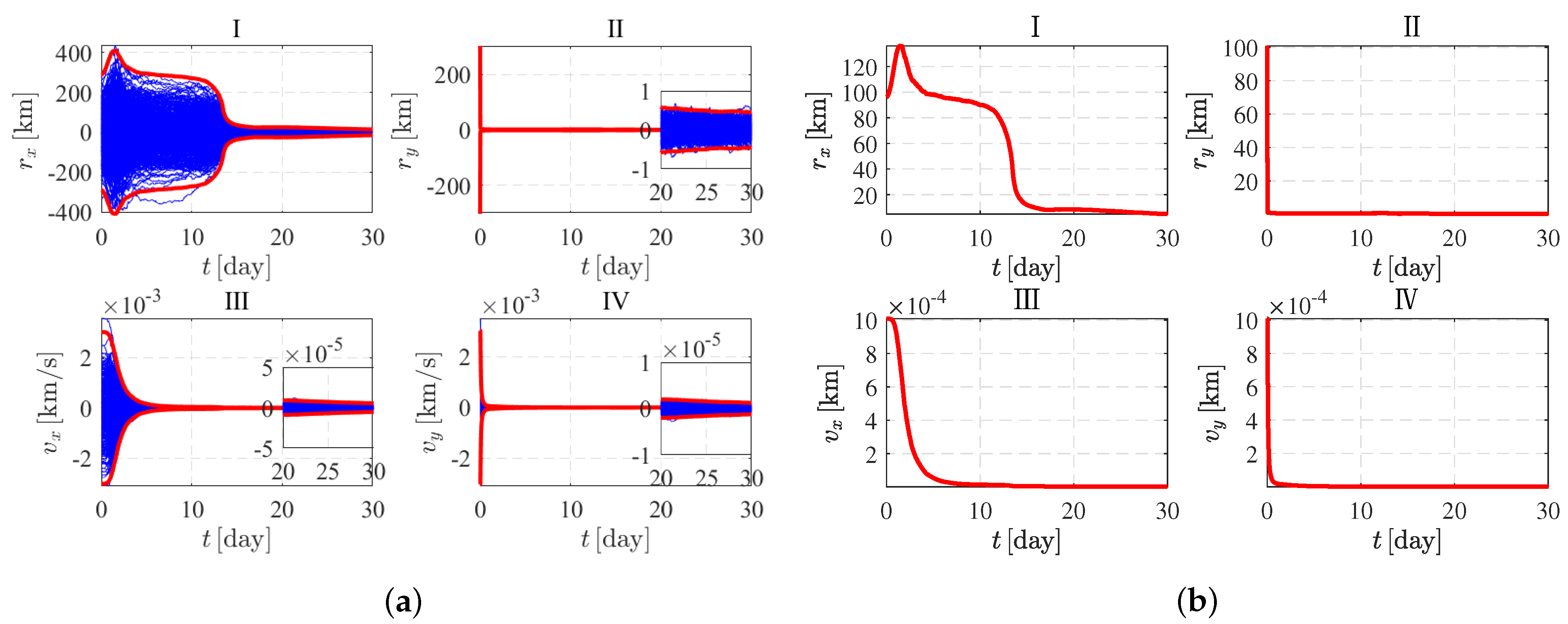
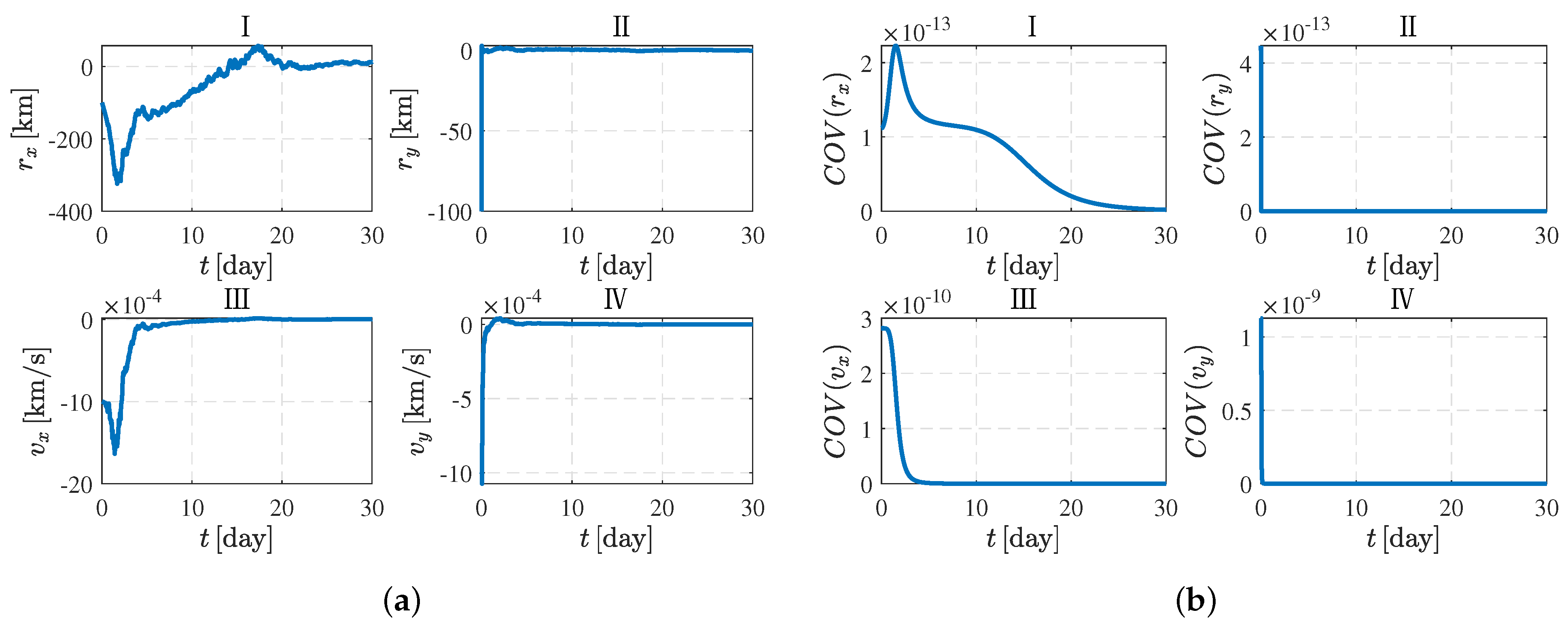
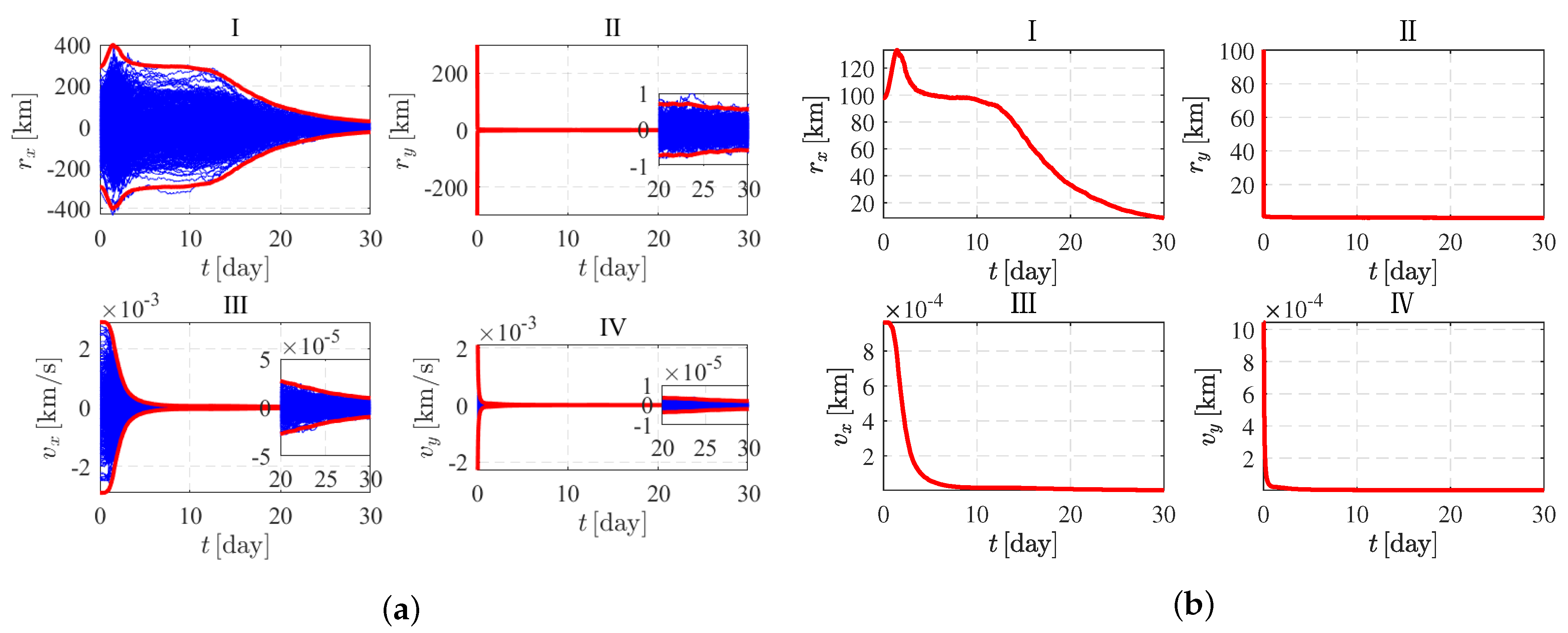
4. Simulation Analysis

In the rotating coordinate system, the controlled periodic orbit is located in the X-Y plane. The amplitude of the periodic orbit along the X direction is 5000 km, and the orbit is composed of four uncontrolled orbital segments in one cycle. The initial parameters and the time of the uncontrolled orbits are shown in

Table 1. Nominal trajectory parameters.

	Position/AU		Velocity/VU
	X	Y	X	Y	Time/h
1	1.01000070094259	−3.34229357677352 × ${10}^{-5}$	8.48460734682508 × ${10}^{-6}$	0.000122175035008374	30
2	1.01000070094259	3.34229357677352 × ${10}^{-5}$	0.000137596252572650	9.87543991711969 × ${10}^{-5}$	30
3	1.01006754681413	3.34229357677352 × ${10}^{-5}$	−8.14563809519688 ×${10}^{-6}$	−0.000122288334314350	30
4	1.01006754681413	−3.34229357677352 × ${10}^{-5}$	−0.000137785577674654	−9.86025641499878 × ${10}^{-5}$	30

. The reference trajectory is shown in Figure 7, together with the measurement curve. It can be seen that the shadow ratio varies from approximately $34.25\%$ to $85.63\%$. Figure 8 shows the contour distribution of the measurement function near the nominal track.

It can be seen that $1\mathrm{th}$ orbital period and $3\mathrm{th}$ orbital period are symmetrical and the $2\mathrm{th}$ orbital period and $4\mathrm{th}$ orbital period are symmetrical. Therefore, the $1\mathrm{th}$ orbital period and $2\mathrm{th}$ orbital period are considered and analyzed below. Firstly, for the $1\mathrm{th}$ orbital period, the simulation is performed by using CKF, where the initial position error is 100 km, the initial speed error is 1 m/s, and the measurement error is 0.001. The simulation results are shown in Figure 9, which, respectively, shows the navigation error and covariance convergence curve. As shown in Figure 9b, the error converges about 15 days later, and the convergence speed of the Y-axis state is faster than that of the X-axis.

Figure 10a shows the 500 times shooting results of the Monte Carlo simulation, in which the accuracy along the X direction is poor and the convergence speed is slow. However, it can be seen that the accuracy in the Y direction is high and the convergence speed is fast. As shown in

Table 2. Analysis of the 3-sigma curve of the $1\mathrm{th}$ orbital period.

	${\mathit{r}}_{\mathit{x}}$/km	${\mathit{r}}_{\mathit{y}}$/km	${\mathit{v}}_{\mathit{x}}$/(km/s)	${\mathit{v}}_{\mathit{y}}$/(km/s)
Initial standard deviation	95.924303	100.433111	0.001004	0.001005
Terminal standard deviation	4.858061	0.151765	0.000002	0.0000004
Convergence percentage	94.9355	99.8489	99.8008	99.9602

, the standard deviation of position error along the X direction is about 4.8581 km and the standard deviation of velocity error is 0.002 m/s. The standard deviation of position error along the Y direction is about 0.1518 km, and the standard deviation of velocity error is 0.0004 m/s.

For the $2\mathrm{th}$ orbital period, the initial position error is 100 km, the initial speed error is 1 m/s, and the measurement error is 0.001. The simulation results are shown in Figure 11, which, respectively, show the navigation error and covariance convergence curve. As shown in Figure 11b, the error converges about 25 days later, and the convergence speed along the Y direction is still faster than along the X direction.

Figure 12a shows the 500 times shooting results of the Monte Carlo simulation, in which the accuracy along the X direction is poor and the convergence speed is slow. However, it is apparent that the accuracy along the Y direction is high and the convergence speed is fast. As shown in

Table 3. Analysis of the 3-sigma curve of the $2\mathrm{th}$ orbital period.

	${\mathit{r}}_{\mathit{x}}$/km	${\mathit{r}}_{\mathit{y}}$/km	${\mathit{v}}_{\mathit{x}}$/(km/s)	${\mathit{v}}_{\mathit{y}}$/(km/s)
Initial standard deviation	97.686914	99.763251	0.000961	0.001001
Terminal standard deviation	8.727596	0.187658	0.000003	0.000001
Convergence percentage	91.0657	99.8119	99.6878	99.9001

, the standard deviation of position error along the X direction is about 8.7276 km and the standard deviation of velocity error is 0.003 m/s. The standard deviation of position error along the Y direction is about 0.1877 km and the standard deviation of velocity error is 0.001 m/s.

5. Conclusions

Aiming at the small-scale orbit near the Sun–Earth L2 point, this paper studied the navigation method based on the Earth-shadow measurement. The paper also considered effects such as the atmosphere and oblateness of the Earth and the Sun in spacecraft autonomous navigation. This method takes the proportion of the Sun blocked by the Earth as the measurement function and calculates the position and velocity of the spacecraft through the continuous change in the measurement function H. For the $1\mathrm{th}$ orbital period, the position error along the X direction is about 4.8581 km and the velocity error is 0.002 m/s. The position error along the Y direction is about 0.1518 km and the velocity error is 0.0004 m/s. For the $2\mathrm{th}$ orbital period, the position error along the X direction is about 8.7276 km and the velocity error is 0.003 m/s. The position error along the Y direction is about 0.1877 km and the velocity error is 0.001 m/s. The above simulation results indicate that the characteristics of convergence and observability along the Y axis are good. Furthermore, this method makes some contribution to the difficulty that the Sun–Earth L2 point has few observations available for navigation and improves the accuracy for autonomous navigation. The autonomous navigation method using satellite-borne equipment has wide application prospects in gravitational wave detection, asteroid exploration, and other deep space exploration fields. Based on this work, the method of autonomous navigation and filtering algorithm could be further conducted in the future.

References

1. Li, C.; Zuo, W.; Wen, W.; Zeng, X.; Gao, X.; Liu, Y.; Fu, Q.; Zhang, Z.; Su, Y.; Ren, X.; et al. Overview of the Chang’e-4 mission: Opening the frontier of scientific exploration of the lunar far side. Space Sci. Rev. 2021, 217, 1–32. [Google Scholar] [CrossRef]
2. Wozniakiewicz, P.J.; Bridges, J.; Burchell, M.J.; Carey, W.; Carpenter, J.; Della Corte, V.; Dignam, A.; Genge, M.J.; Hicks, L.; Hilchenbach, M.; et al. A cosmic dust detection suite for the deep space Gateway. Adv. Space Res. 2021, 68, 85–104. [Google Scholar] [CrossRef]
3. Cui, P.; Qin, T.; Zhu, S.; Liu, Y.; Xu, R.; Yu, Z. Trajectory curvature guidance for Mars landings in hazardous terrains. Automatica 2018, 93, 161–171. [Google Scholar] [CrossRef]
4. Qin, T.; Zhu, S.; Cui, P.; Luan, E. Divert capability analysis and subsequent guidance design for mars landing. In Proceedings of the 2018 IEEE Aerospace Conference, Big Sky, MN, USA, 4–11 March 2018; pp. 1–15. [Google Scholar]
5. Beckman, M. Orbit determination issues for libration point orbits. In Libration Point Orbits and Applications; World Scientific: Singapore, 2003; pp. 1–17. [Google Scholar]
6. Cao, J.; Hu, S.; Huang, Y.; Liu, L. Orbit determination and analysis for chang’E-2 extended mission. Geomat. Inf. Sci. Wuhan Univ. 2013, 38, 1339–1343. [Google Scholar]
7. Bobrinksy, N.; Maldari, P.; Schulz, K.J.; Sessler, G.; Mascaraque, Í. ESA’s Space Communication Architecture and Ground Station Evolution. In Proceedings of the SpaceOps 2008 Conference, Heidelberg, Germany, 12–16 May 2008; p. 3237. [Google Scholar]
8. Barriot, J.; Serafini, J.; Sichoix, L. Calibration of the KA Band Tracking of the Bepi-Colombo Spacecraft (more Experiment). In Proceedings of the AGU Fall Meeting Abstracts, San Francisco, CA, USA, 9–13 December 2013; Volume 2013, p. P13A-1743. [Google Scholar]
9. Huang, Y.; Li, P.; Fan, M. Orbit determination of CE-5T1 in Earth-Moon L2 libration point orbit with ground tracking data. 42nd COSPAR Sci. Assem. 2018, 42, B3-1. [Google Scholar] [CrossRef]
10. Li, X.; Sanyal, A.K.; Warier, R.R.; Qiao, D. Landing of Hopping Rovers on Irregularly-shaped Small Bodies Using Attitude Control. Adv. Space Res. 2020, 65, 2674–2691. [Google Scholar] [CrossRef]
11. Li, X.; Qiao, D.; Barucci, M. Analysis of equilibria in the doubly synchronous binary asteroid systems concerned with non-spherical shape. Astrodynamics 2018, 2, 133–146. [Google Scholar] [CrossRef]
12. Zhou, X.; Cheng, Y.; Qiao, D.; Huo, Z. An adaptive surrogate model-based fast planning for swarm safe migration along halo orbit. Acta Astronaut. 2022, 194, 309–322. [Google Scholar] [CrossRef]
13. Qin, T.; Zhu, S.; Cui, P.; Gao, A. An innovative navigation scheme of powered descent phase for Mars pinpoint landing. Adv. Space Res. 2014, 54, 1888–1900. [Google Scholar] [CrossRef]
14. Luo, Y.; Qin, T.; Zhou, X. Observability Analysis and Improvement Approach for Cooperative Optical Orbit Determination. Aerospace 2022, 9, 166. [Google Scholar] [CrossRef]
15. Zhou, X.; Qin, T.; Meng, L. Maneuvering Spacecraft Orbit Determination Using Polynomial Representation. Aerospace 2022, 9, 257. [Google Scholar] [CrossRef]
16. Vasile, M.; Sironi, F.; Bernelli-Zazzera, F. Deep space autonomous orbit determination using CCD. In Proceedings of the AIAA/AAS Astrodynamics Specialist Conference and Exhibit, Monterey, CA, USA, 5–8 August 2002; p. 4818. [Google Scholar]
17. Yim, J.R.; Crassidis, J.L.; Junkins, J.L. Autonomous orbit navigation of two spacecraft system using relative line of sight vector measurements. In Proceedings of the AAS Space Flight Mechanics Meeting, Maui, HI, USA, 8–12 February 2004. [Google Scholar]
18. Chang, W.; Gan, Q.; Zhang, J.; Lu, B.; Ma, J. An orbit determination method using space-based angle measured data. Acta Astron. Sin. 2008, 49, 81–92. [Google Scholar]
19. Zhang, J.; Cai, W.; Sun, C. Monocular vision-based relative motion parameter estimation for non-cooperative objects in space. Aerosp. Control Appl. 2010, 36, 31–35. [Google Scholar]
20. Liu, G. Research on Non-Cooperative Target Tracking Algorithms and Related Technologies Using Space-Based Bearings-Only Measurements, Graduate School of National University of defence Technology; Graduate School of National University of Defense Technology: Singapore, 2011; pp. 26–30. [Google Scholar]
21. Lu, R. Study on Autonomous Optical Navigation Technology for Deep Space Probe; Graduate School of Nanjing University of Aeronautics and Astronautics: Nanjing, China, 2013. [Google Scholar]
22. Wang, Y.; Zhang, Y.; Qiao, D.; Mao, Q.; Jiang, J. Transfer to near-Earth asteroids from a lunar orbit via Earth flyby and direct escaping trajectories. Acta Astronaut. 2017, 133, 177–184. [Google Scholar] [CrossRef]
23. Cui, P.; Qiao, D.; Cui, H.; Luan, E. Target selection and transfer trajectories design for exploring asteroid mission. Sci. China Technol. Sci. 2010, 53, 1150–1158. [Google Scholar] [CrossRef]
24. Silvestrini, S.; Piccinin, M.; Zanotti, G.; Brandonisio, A.; Lunghi, P.; Lavagna, M. Implicit Extended Kalman Filter for Optical Terrain Relative Navigation Using Delayed Measurements. Aerospace 2022, 9, 503. [Google Scholar] [CrossRef]
25. Chen, J.; Jiao, W.; Ma, J.; Song, X. Autonav of navigation satellite constellation based on crosslink range and orientation parameters constraining. Geomat. Inf. Sci. Wuhan Univ. 2005, 30, 439–443. [Google Scholar]
26. Li, X.; Qiao, D.; Li, P. Frozen orbit design and maintenance with an application to small body exploration. Aerosp. Sci. Technol. 2019, 92, 170–180. [Google Scholar] [CrossRef]
27. Channumsin, S.; Jaturutd, S. Analysis of coupled attitude and orbit dynamics for uncontrolled re-entry satellite. In Proceedings of the 2019 7th International Electrical Engineering Congress (iEECON), Cha-am, Thailand, 6–8 March 2019; pp. 1–4. [Google Scholar]
28. Li, X.; Warier, R.R.; Sanyal, A.K.; Qiao, D. Trajectory tracking near small bodies using only attitude control. J. Guid. Control. Dyn. 2019, 42, 109–122. [Google Scholar] [CrossRef]
29. Tang, C.; Hu, X.; Zhou, S.; Liu, L.; Pan, J.; Chen, L.; Guo, R.; Zhu, L.; Hu, G.; Li, X.; et al. Initial results of centralized autonomous orbit determination of the new-generation BDS satellites with inter-satellite link measurements. J. Geod. 2018, 92, 1155–1169. [Google Scholar] [CrossRef]
30. Wang, Y.; Qiao, D.; Cui, P. Design of optimal impulse transfers from the Sun–Earth libration point to asteroid. Adv. Space Res. 2015, 56, 176–186. [Google Scholar] [CrossRef]
31. Xu, L.; Zhao, X.; Guo, L. An autonomous navigation study of Walker constellation based on reference satellite and inter-satellite distance measurement. In Proceedings of the 2014 IEEE Chinese Guidance, Navigation and Control Conference, Yantai, China, 8–10 August 2014; pp. 2553–2557. [Google Scholar]
32. Qin, T.; Qiao, D.; Macdonald, M. Relative orbit determination using only intersatellite range measurements. J. Guid. Control. Dyn. 2019, 42, 703–710. [Google Scholar] [CrossRef]
33. Edery, A. Earth Shadows and the SEV Angle of MAP’s Lissajous Orbit at L2. In Proceedings of the AIAA/AAS Astrodynamics Specialist Conference and Exhibit, Monterey, CA, USA, 5–8 August 2002; p. 4428. [Google Scholar]
34. Adhya, S.; Sibthorpe, A.; Ziebart, M.; Cross, P. Oblate earth eclipse state algorithm for low-earth-orbiting satellites. J. Spacecr. Rocket. 2004, 41, 157–159. [Google Scholar] [CrossRef]
35. Qiao, D.; Cui, P.; Cui, H. Proposal for a multiple-asteroid-flyby mission with sample return. Adv. Space Res. 2012, 50, 327–333. [Google Scholar] [CrossRef]
36. Soto, G.; Savransky, D.; Gustafson, E.; Shapiro, J.; Keithly, D.; Della Santina, C. Navigation and Orbit Phasing of Modular Spacecraft for Segmented Telescope Assembly about Sun-Earth L2. In Proceedings of the American Astronomical Society Meeting Abstracts# 233, Seattle, WA, USA, 6–10 January; Volume 233, p. 157.20.
37. Wang, Y.M.; Qiao, D.; Cui, P.Y. Design of low-energy transfer from lunar orbit to asteroid in the Sun-Earth-Moon system. Acta Mech. Sin. 2014, 30, 966–972. [Google Scholar] [CrossRef]
38. Canalias, E.; Gomez, G.; Marcote, M.; Masdemont, J. Assessment of Mission Design Including Utilization of Libration Points and Weak Stability Boundaries; ESA Advanced Concept Team: Noordwijk, The Netherlands, 2004. [Google Scholar]
39. Farquhar, R.W.; Dunham, D.W.; Guo, Y.; McAdams, J.V. Utilization of libration points for human exploration in the Sun–Earth–Moon system and beyond. Acta Astronaut. 2004, 55, 687–700. [Google Scholar] [CrossRef]
40. Zhang, R.; Tu, R.; Zhang, P.; Liu, J.; Lu, X. Study of satellite shadow function model considering the overlapping parts of Earth shadow and Moon shadow and its application to GPS satellite orbit determination. Adv. Space Res. 2019, 63, 2912–2929. [Google Scholar] [CrossRef]
41. Srivastava, V.K.; Yadav, S.; Kumar, J.; Kushvah, B.; Ramakrishna, B.; Ekambram, P. Earth conical shadow modeling for LEO satellite using reference frame transformation technique: A comparative study with existing earth conical shadow models. Astron. Comput. 2015, 9, 34–39. [Google Scholar] [CrossRef]
42. Wang, Y.; Topputo, F. Indirect Optimization for Low-Thrust Transfers with Earth-Shadow Eclipses. In Proceedings of the 31st AAS/AIAA Space Flight Mechanics Meeting, Charlotte, NC, USA, 31 January–4 February 2021; pp. 1–17. [Google Scholar]
43. Toulmonde, M. The diameter of the Sun over the past three centuries. Astron. Astrophys. 1997, 325, 1174–1178. [Google Scholar]
44. Li, Z.; Ziebart, M.; Bhattarai, S.; Harrison, D. A shadow function model based on perspective projection and atmospheric effect for satellites in eclipse. Adv. Space Res. 2019, 63, 1347–1359. [Google Scholar] [CrossRef] [Green Version]
Figure 1. Circular Restricted Three-body Problem.
Applsci 12 12154 g001
Figure 2. Schematic diagram of Lagrange point between the Sun and the Earth.
Applsci 12 12154 g002
Figure 3. The model considering the atmosphere and oblateness of the Earth and the Sun.
Applsci 12 12154 g003
Figure 4. Schematic diagram of Earth-shadow area.
Applsci 12 12154 g004
Figure 5. Measurement model of Earth shadow.
Applsci 12 12154 g005
Figure 6. Three types of Earth-shadow. (a) Occlusion situation 1. (b) Occlusion situation 2. (c) Occlusion situation 3.
Applsci 12 12154 g006
Figure 7. Nominal trajectory and its measurement parameters. (a) Nominal trajectory. (b) Measurement curve.
Applsci 12 12154 g007
Figure 8. Contour lines of measurements near the nominal track. (a) Outline of the nominal track. (b) Contour map of the nominal track.
Applsci 12 12154 g008
Figure 9. Navigation error results and covariance convergence curve. (a) Navigation error. (b) Covariance convergence curve.
Applsci 12 12154 g009
Figure 10. Results of the Monte Carlo simulation of the 1 th orbital period. (a) 500 times shooting results. (b) 3-sigma curve.
Applsci 12 12154 g010
Figure 11. Navigation error results and covariance convergence curve. (a) Navigation error. (b) Covariance convergence curve.
Applsci 12 12154 g011
Figure 12. Results of the Monte Carlo simulation of the 2 th orbital period. (a) 500 times shooting results. (b) 3-sigma curve.
Applsci 12 12154 g012