HTN: Hybrid Transformer Network for Curvature of Cervical Spine Estimation

Abstract

Many young people have suffered from cervical spondylosis in recent years due to long-term desk work or unhealthy lifestyles. Early diagnosis is crucial for curing cervical spondylosis. The Cobb angle method is the most common method for assessing spinal curvature. However, manually measuring the Cobb angle is time-consuming and heavily dependent on personal experience. In this paper, we propose a fully automatic system for measuring cervical spinal curvature on X-rays using the Cobb angle method, which can reduce the workload of clinicians and provide a reliable basis for surgery. Hybrid transformer network (HTN) blends a self-attention mechanism, self-supervision learning, and feature fusion. In addition, a new cervical spondylosis dataset is proposed to evaluate our method. Our model can achieve a SMAPE of 11.06% and a significant Pearson correlation coefficient of 0.9619 (p < 0.001) on our dataset. The absolute difference between the ground truth and the prediction obtained is less than 2°, implying clinical value. Statistical analysis proves the reliability of our method for Cobb angle estimation. To further prove the validity of our method, the HTN was also trained and evaluated on the public AASCE MICCAI 2019 challenge dataset. The experimental results show that our method can achieve comparable performance to state-of-the-art methods, which means that our method can measure the curvature of the neck and the entire spine.

1. Introduction

Cervical spondylosis is one of the top ten chronic diseases in the world, which can trigger neck pain, arm pain, numbness, and limited neck movement, seriously affecting people’s lives and work [1]. In previous decades, it more frequently occurred in middle-aged and elderly people. However, with the popularization of electronic products and long-term poor sitting posture for desk-work and study, the mean age of onset has shown a younger trend in recent years. Therefore, analysis of the cervical spine has become a hotspot in medical-image processing.

Abnormal cervical spine curvature is often the first imaging feature of cervical spine degeneration. Therefore, cervical spinal curvature is a widespread clinical method for assessing the state of the cervical spine [2]. Accurate measurement and analysis of cervical spine curvature can provide an essential reference and basis for the early diagnosis of cervical spondylosis. They also play a crucial role in the preoperative evaluation of cervical spine biomechanics research. The Cobb angle method is common for assessing cervical spinal curvature because it is easier to perform and has better reliability within, and between, groups than other methods. Presently, clinicians still manually measure the Cobb angle or use specific computer-assisted tools and software to perform measurements [3,4,5]. However, these methods are not automatic since observers need to draw lines or landmarks on online X-rays manually. These methods are also tedious and time-consuming, and errors caused by subjective factors may occur [6].

To implement automated spine image analysis, a growing body of research has employed deep-learning technology to process images for diagnosis automatically. Recently, some pioneers [6,7,8,9,10,11,12,13,14,15,16] have applied landmark detection methods to the field of spinal images. MVC-Net [16] creatively designed multi-view convolution layers to extract global spinal information by aggregating multi-view features from both AP and LAT X-rays. Based on this idea, MVE-Net [7] proposed an error-controlled loss function to speed up convergence and achieve high accuracy. AEC-Net [8] used a large convolutional kernel to learn the boundary features of spines, which a landmark detector then used to regress landmarks. Bayat et al. [17] introduced the residual corrector component to correct the location and landmark estimations. Spatial Configuration Net [11] generated the location of the target landmark by multiplying the local appearance and spatial configuration.

Nevertheless, existing studies [6,7,8,9,10,11,12,13,14,15,16] on the Cobb angle only use the symmetric mean absolute percentage error (SMAPE) as the evaluation index. SMAPE is the officially announced evaluation method for this dataset. However, it is not sufficient from a clinical point of view. The value of SMAPE is not intuitive compared with the angle. We propose more performance metrics in our work to evaluate the model’s performance, such as mean absolute difference, Bland–Altman difference diagrams, and Pearson correlation coefficient.

In addition, CNNs have been widely used for various segmentation-related tasks and achieved encouraging performance in medical-image segmentation in the past decade. We have witnessed the remarkable success of fully convolutional networks [18], U-Net [19], and their variants [20]. Both architectures benefit from the encoder–decoder structure. However, they fail to build long-range dependencies and global contexts in images; this impacts the further improvement of segmentation accuracy due to the limitation of the receptive field in convolution operation and the inherent inductive biases presented in the convolutional architectures. Generally, a transformer can solve the problem of global dependencies. Although the transformer was originally designed for sequence-to-sequence modeling in natural language processing (NLP) models, now it is generally considered a more flexible alternative to CNNs for processing various vision tasks. Deep-natural networks with transformers perform better than those without transformers in many visual benchmarks. Inspired by the powerful presentation capabilities of transformers, transformers have been introduced into medical-image segmentation and achieve fantastic performance [20,21,22,23]. Chen J et al. [24] and Wang W et al. [25] use transformers to extract global contexts in medical-image segmentation.

Inspired by [24,25], we propose a hybrid transformer network, which leverages the high-level semantic features provided by the encoding network, the fine-grained features provided by the decoding network, and the global dependencies provided by the transformer to learn the feature representation of the entire spine. Most previous works stack a transformer on top of the CNN backbone, which undoubtedly increases the number of calculations and reduces the network speed. Therefore, in this work, we only add the transformer module to the last layer of the encoder network, which alleviates the problem of increased computation due to the addition of the transformer.

To our knowledge, existing works have no open-access medical-image dataset of the cervical vertebrae area. There are relatively few studies on the diagnosis of cervical spine imaging. This paper presents a novel automatic system for estimating cervical spinal curvature to overcome these limitations and to fully utilize deep-learning technology, which can achieve comparable performance to experts. Our method will inspire many people who are interested in this field. The code will be released at: https://github.com/JiuqingDong/Curvature-of-Cervical-Spine-Estimation (accessed on 25 November 2022).

The key contributions of our method are presented as follows:

• We propose a hybrid network that blends a self-attention mechanism, self-supervision learning, and feature fusion, which can accurately estimate the Cobb angle, analyze the curvature of the cervical spine, and provide reliable information for cervical diagnosis. Many evaluation metrics are used to evaluate our methods. Our method achieves a highly significant correlation of 0.9619 (p < 0.001) with the ground truth, with a small mean absolute difference of 1.79°. To a certain extent, our method can provide a reasonably reliable basis for clinicians and surgical navigation.
• A new dataset is proposed to evaluate our method for spondylosis detection. The dataset was annotated by one spine surgeon and proofread by another expert. To the best of our best knowledge, it is the first study using cervical spine-region X-ray images to estimate the Cobb angle by using a hybrid transformer network. Furthermore, the AASCE MICCAI 2019 challenge dataset is also used to evaluate our method. The experimental results show that our method can achieve performance comparable to state-of-the-art methods, which proves the generalization of our method.
• We compare methods of combining transformers with encoder–decoder networks and discuss transfer learning in medical-image processing tasks. In conclusion, this original article lays a foundation for estimating the cervical Cobb angle, inspiring subsequent works in the related domains.

2. Materials and Methods

2.1. Datasets

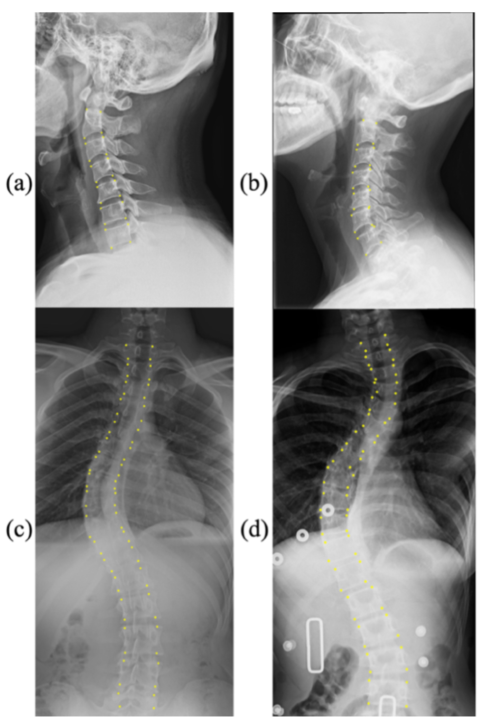
Two datasets are used to evaluate the superiority of our proposed method: our dataset and the public AASCE MICCAI 2019 challenge dataset. Figure 1 shows a few samples with corresponding landmarks of these two datasets. More details are presented as follows:

CS799 dataset: Our dataset contains a total of 799 LAT X-ray images of the cervical spine. All the samples were captured from 799 distinct human subjects. The subjects in this dataset exhibit a wide age distribution (from 12 to 84 years), and the average age is 45.3 years. The curvature of the cervical spine is also diverse. The Cobb angles are distributed between 0° and 46.3°. The cervical spine has a unique vertebral appearance. All images were collected by Shanghai ChangZheng Hospital, annotated, and proofread by spine surgery specialists. The minimum resolution of the picture is 1217 × 1779, while the maximum resolution is 1916 × 2695. We trained our models on the training dataset with 559 images (75%), of which 159 images were used for validation (15%), and 81 images werew used for testing (10%). Each image includes 24 landmarks.

AASCE MICCAI 2019 challenge dataset: Each X-ray image has 68 landmarks corresponding to 17 vertebrae. Each vertebra includes four corner landmarks (top-left, top-right, bottom-left, and bottom-right). The challenge also supplies Cobb angles for proximal thoracic (PT), main thoracic (MT), and thoracolumbar (TL). In the same way as the data was split in [9], we divided the dataset into three parts: 348 images for training (60%), 116 images for validation (20%), and 116 images for testing (20%).

It is noteworthy that the division ratios of the two datasets are different. The division of the public dataset is consistent with previous methods. For our dataset CS799, we tried to use more samples for training, which may have caused some doubts. However, the focus of this paper is to verify the effectiveness of our proposed module. Therefore, the division of the dataset does not affect the conclusion.

2.2. Overall Framework

Our model design is based on an encoder–decoder structure. The encoding path mainly consists of several residual blocks. In contrast, the decoding path is divided into two branches to up-sample the feature maps. The first branch is the main decoding path, and the second branch is the intermediate branch. The main decoding path uses a traditional up-sampling process. In particular, the structure of the intermediate branch is similar to that of the main decoding path, but their inputs are different. The intermediate branch reuses the features in the encoder and uses the loss function for backpropagation to optimize the parameters. Inspired by self-supervision learning [26], we add the hybrid-loss function in the network. Specifically, we not only utilize the feature map of the last layer of the decoder to predict landmarks but also use the feature map of the last layer of the intermediate branch to assist in prediction. On this basis, our primary decoder uses the feature information learned by the intermediate branch to capture more representative features and to reduce the acquisition of invalid information from the encoder.

A prediction module is utilized to detect landmarks of the spine. This module can generate a heatmap, an offset map of center points, and a centripetal vector map. Through the arithmetic addition between the heatmap and the offset map, we obtain the coordinates of the center points. Our goal is to obtain landmarks, so we use the coordinates of the center points to subtract the centripetal vector to obtain the set of corner coordinates. Afterward, the Cobb angle can be obtained by a geometric algorithm.

In addition, we merge the feature maps of different layers of the main decoding path to obtain the fusion feature map. Feature fusion can optimize the model’s parameters and improve landmark detection accuracy, leading to a precise Cobb angle. The overall framework of our method is shown in Figure 2.

We also wondered which hybrid structure would lead to better performance. Therefore, we explored the impact of introducing a transformer earlier in the encoder–decoder network on the final model. In other words, we removed residual module 1 in the encoder–decoder (Shown in Figure 2), which resulted in a larger size of feature maps processed by the transformer. We compare the performance of the two models in Section 3.4.

2.3. Integration of Transformer

Given the input image $X\in R^{H_0\ast W_0\ast 3}$ with a spatial resolution of $H_0\ast W_0$ and three-color channels, our designed down-sampling path generates the high-level feature representation $X\in R^{H\ast W\ast C}$. Here we use $C=512$ and $H,W=H_0/32,W_0/32$. The feature representation $F$ is fed to the main decoding path and intermediate branch. Before decoding, a transformer is integrated.

To perform tokenization, we uniformly slip the feature representation F into a sequence of flattened 2D patches $x_F\left\{x_F^i\in R^{N\ast \left(P^2\ast C\right)}|i=1,\dots ,N\right\}$, where the size of each patch is ${\mathrm{P}}^2$ and $\mathrm{N}=\mathrm{H}\ast \mathrm{W}/{\mathrm{P}}^2$ is the resulting number of patches. The transformer expects a 1D sequence of token embeddings as input; hence, we flatten the 2D patches into 1D and map it into a D-dimensional embedding space using a trainable linear projection. Moreover, we add a learnable 1D position embedding to the patch embeddings to preserve the positional information. The obtained embedding vector sequence is utilized as the input of the encoder, as shown in Equation (1):

$$Y_0=\left[x_F^{1}E; x_F^{2}E; \dots ;x_F^{N}E; \right]+E_{pos}$$

(1)

where $E\in R^{P^2\ast C\ast D}$ is the linear projection matrix, $E_{pos}\in R^{N\ast D}$ is the position embedding, and $Y_0$ is the final feature embedding. The output of this projection is regarded as the patch embedding.

In general, a transformer includes an encoder and a decoder. In its encoding path, there are $L$ alternating layers, each of which consists of multi-head self-attention (MHSA) and multilayer perceptron (MLP) blocks. A residual connection is added to the input and output of each module, and layer normalization is applied before every block. In addition, each MLP block contains two layers with GELU nonlinearity. Therefore, the output of the $l$-th layer can be expressed as Equations (2) and (3):

$${\widehat{Y}}_l=MHSA\left[LN\left(Y_{l-1}\right)\right]+Y_{l-1}$$

(2)

$$Y_l=MLP\left[LN\left({\widehat{Y}}_l\right)\right]+{\widehat{Y}}_l$$

(3)

where $LN\left(\ast \right)$ refers to the layer normalization operator, the output of the $l$-th layer is $Y_l$, and $l\in \left[1,2,\dots ,L\right]$. In our experiments, $L=4$.

The multi-head self-attention block is the most important part in the transformer. Multiple self-attention modules are processed, connected, and projected in parallel. The inputs $x_F$ are transformed into three parts: the $d_k$-dimension queries $Q$, $d_k$-dimension keys $K,$ and $d_v$-dimension values $V$. All of them have the same sequence length as the inputs $x_F$. The scaled dot-product attention is applied as follows:

$$Attn\left(Q,K,V\right)=softmax\left(\raisebox{1ex}{$Q{K}^T$}\!\left/ \!\raisebox{-1ex}{$\sqrt{d_k}$}\right.\right)\ast V$$

(4)

The decoder of the transformer also consists of $L$ identical layers, but it inserts an additional multi-head layer that pays more attention to the output of the encoder stack. A residual connection is added to its input and output, similar to the operation outside each module, and layer normalization is applied.

To predict landmarks of the spine, we use a 2D CNN to restore the spatial order and to map the serialized data back to the feature map. Specifically, the $D$-dimensional output sequence of transformer $Y_L\in R^{N\ast L}$ is projected back to the $C$-dimension through a linear projector. We obtain the feature map $Y\in R^{H\ast W\ast C}$ with the same size of the feature representation $F$. After feature mapping, we stack the up-sampling layer and convolutional layer to decode the hidden feature for landmark prediction. Although they have similar structures, the two branches have their own functions. The intermediate branch is developed to enhance the feature learned from the encoder, while the main decoding path once again strengthens the learning content of the intermediate branch.

2.4. Prediction Module

The prediction module is composed of multiple branches for generating the center heatmap, center offset and centripetal vector. Each branch consists of two convolutional layers. We use ReLU as the activation function of the first layer.

The method for generating the center heatmap is the same as that employed for human pose estimation [27]. For each point, there is only one positive position; the remaining positions are negative. Therefore, we reduce the penalty for incorrect positions within the radius of the correct position to reduce the imbalance between positive samples and negative samples. We assume that the coordinates of the center point are $\left(i,j\right)$ and that the reduction of penalty is given by a Gaussian kernel, as shown in Equation (5):

$$G\left(i,j\right)=e^{-\frac{i^2+j^2}{2{\sigma }^2}}$$

(5)

where $\mathsf{\sigma }$ is a standard deviation that depends on the size of the vertebrae. Each center corresponds to a vertebra. We take the maximum when two center points overlap.

The predicted landmarks may deviate from their previous positions when they are mapped back to the original image, so offsets are designed to compensate for location errors. If the center point is located at $\left(i,j\right)$, the corresponding coordinate in the downsized feature map $Y$ is $\left(\frac{i}{n},\frac{j}{n}\right)$, where $n$ is the down-sampling factor. In our experiment, $n=4$ because the feature maps from the decoder are a quarter of the original X-ray images. The center offset is $\delta =\left(\frac{i}{n}-{\left[\frac{i}{n}\right]}^{\prime },\frac{j}{n}-{\left[\frac{j}{n}\right]}^{\prime }\right)$. Each X-ray image has $m$ 2D coordinates of spinal centers, so there are $m\ast 2$ channels in the center offset map.

The centripetal vector is defined as a vector starting from the center of the vertebra and pointing to four corners of each vertebra. Each vertebra has coordinates of 4 vectors pointing to the center, and there is a total of $m$ vertebrae. Therefore, the centripetal vector map has $m\ast 8$ channels. We use the predicted center point to subtract the centripetal vector to obtain the final coordinates of the corner points. If the corners belong to the same vertebra, the network will predict similar embedding for them. In this way, we can retain the order of the landmarks.

2.5. Feature Fusion

To enhance features, feature fusion is applied in the model, which can help deep-network training and improve the prediction quality of heatmaps. On each layer of the main decoding path, the model generates one auxiliary prediction output (heatmap). Then the three feature maps with different sizes are fused. As shown in Figure 2, the model implements self-supervision on several maps by using the same prediction module to predict landmarks and calculate the final loss, so that it can improve the performance of the model. This training method can provide more supervision information, which is more conducive to the improvement of network performance than only calculating the loss in the output layer.

2.6. Hybrid Loss

We propose a hybrid-loss function to train our end-to-end network for landmark detection. The overall loss function can be described as (6)

$$L=L_{cthm}+L_{ctoffset}+L_{vec}$$

(6)

where $L_{cthm}$, $L_{ctoffset}$ and $L_{vec}$ refer to the loss of the center heatmap, center offset and centripetal vector, respectively.

We choose focal loss to optimize the center heatmap, and $L1$ loss is used to train the center offset and centripetal vector. Specifically, the focal loss is defined as (7):

$$L_{cthm}=L_{FL}=-\frac{1}{N}{{\displaystyle \sum }}_{ij}\left\{\begin{array}{ll}{\left(1-p_{ij}\right)}^{\alpha }log{p}_{ij}& g_{ij}=1\\ {\left(1-g_{ij}\right)}^{\beta }{\left(p_{ij}\right)}^{\alpha }log\left(1-p_{ij}\right)& others\end{array}\right.$$

(7)

where $p_{ij}$ refers to the scores of the prediction at location $\left(i,j\right)$ and the ground truth of the corresponding position is recorded as $g_{ij}$. We set the hyperparameter $\alpha$ = 2 and 𝛽 = 4. $N$ refers to the number of positions on the feature map. The L₁ loss is formulated as:

$$L_{ctoffset}=L_{vec}=L_{l1}=\frac{1}{N}{{\displaystyle \sum }}_{k=1}^N{L}_1\left(\sigma ,\widehat{\sigma }\right)$$

(8)

where $N$ is the number of coordinates, $\mathsf{\sigma }$ refers to the prediction of the offset, and $\mathsf{\sigma } ^$ is the ground truth of the offset.

3. Experiments

3.1. Training Details

We implemented our method in Pytorch 1.10 with python 3.7 on GTX 3090 GPU. The initial learning rate was set to 1.25 × 10⁻³ using an exponential schedule with a decay rate of 0.96. Other weights of the network were initialized from a standard Gaussian distribution. The network was trained for 80 epochs with a batch size of 4 and stopped when the validation loss did not decrease significantly. The model with the minor validation loss was used to evaluate our method on the test dataset. In addition, we applied standard data augmentation, such as cropping, random expansion, contrast, and brightness distortion. We fixed the input resolution of the images to 1024 × 512, which gives an output resolution of 256 × 128. For the CS799 dataset, we set each image to predict six vertebrae with 24 key points. For the AASCE Challenge dataset, we used 68 key points to predict 17 vertebrae. Cobb angle could automatically be computed by using the law of cosines.

3.2. Evaluation Metrics

We evaluated the accuracy of the landmarks by comparing the coordinates of labels and predictions. The mean square error (MSE) is defined as (9):

$$MSE=\frac{1}{N}{{\displaystyle \sum }}_{i=1}^N{(p_{ij}-g_{ij})}^2$$

(9)

where $N$ is the total number of landmarks, $p_{ij}$ denotes the predicted landmarks at location $\left(i,j\right)$, and $g_{ij}$ is the ground truth.

For Cobb angle estimation, symmetric mean absolute percentage error (SMAPE) was used to evaluate the results and is defined as follows:

$$SMAPE=\frac{1}{M}{{\displaystyle \sum }}_{i=1}^M\frac{\left|A-B\right|}{\left(\left|A\right|+\left|B\right|\right)/2}\ast 100\%$$

(10)

where $M$ is the number of testing images, $A$ is the ground truth of the Cobb angle and $B$ is the prediction.

Statistical analysis was implemented to quantitatively analyze the difference between the predicted value and the ground truth. We provided the performance metrics, including mean absolute difference (MAD) and corresponding standard deviation (SD). The Pearson correlation coefficient (R) between the predicted Cobb angle and the annotated ground truth was computed as:

$$R=\frac{cov\left(A,B\right)}{\sigma A\sigma B}$$

(11)

where $A$ is the ground truth of the Cobb angle and $B$ is the prediction.

3.3. Ablation Study

Our model achieved a Pearson correlation coefficient of R = 0.9619 (p < 0.001), which means that the prediction of our method has high consistency with the ground truth. In other words, the Cobb angle estimated by our method highly correlates with that measured by experts. The SMAPE of our model is 11.06%. We also show the results of a student’s paired t-test. The significance level in hypothesis testing was set to 0.05. No statistically significant differences were observed between the measurement of our method and the manual method since the p-value is greater than 0.05 (p = 0.876).

To thoroughly validate the effectiveness of our model, various ablation studies were performed. We analyzed the effect of our encoder–decoder structure, transformer module, intermediate branch, and self-supervision learning. As shown in

Table 1. Ablation studies of each component of our model. ED (encoder–decoder network); SE (SE attention); TM (transformer module); IB&FF (intermediate branch and feature fusion); HL (hybrid loss); SMAPE (symmetric mean absolute percentage error); MAD (mean absolute difference; SD (standard deviation); Confidence 95% (confidence interval of the difference of the statistic); R (Pearson correlation coefficient); MSE (mean square error). All ablation study experiments were conducted on the CS799 dataset.

ED	SE	TM	IB & FF	HL	SMAPE (%)	MAD (SD)	Confidence	R (p-Value)	MSE
P					14.25	2.26° (1.90°)	5.98°	0.9501 (<10−6)	5.97
P				P	12.58	2.14° (1.87°)	5.81°	0.9527 (<10−6)	5.84
P			P	P	12.37	2.11° (1.93°)	5.90°	0.9526 (<10−6)	5.24
P		P	P	P	11.06	1.79° (1.86°)	5.45°	0.9619 (<10−6)	5.24
P	P	P	P	P	12.55	1.92° (2.57°)	4.71°	0.9611 (<10−6)	5.46
P	P				13.45	2.08° (2.73°)	5.72°	0.9538 (<10−6)	5.53
P	P		P	P	11.83	1.91° (2.50°)	4.85°	0.9638 (<10−6)	5.26

, with the simple encoder–decoder structure, our model achieved a SMAPE of 14.25%, an MAD (SD) of 2.26° (2.84°), a Pearson correlation coefficient of 0.9501 (p < 0.001), and an MSE of 6.01. When adding self-supervision, we obtained 12.58%, 2.14° (2.77°), 0.9527 (p < 0.001), and 5.84 in terms of SMAPE, MAD (SD), Pearson correlation coefficient, and MSE, respectively. Subsequently, an intermediate branch was added. All indicators exhibited an improving trend. We were able to obtain the lowest SMAPE of 11.06%, the smallest mean absolute difference, the narrowest confidence interval of the difference, a higher Pearson correlation coefficient of 0.9619 (p < 0.001), and the smallest MSE of 5.24 in our final model.

In addition, we also used SE attention [28] instead of the transformer to determine how different attention mechanisms affected the model. Ablation studies about SE attention were also conducted (refer to the last three rows of Table 1). We observed that SE attention could also improve the model’s performance. Nevertheless, compared with the transformer, this performance gain was slightly smaller.

We explored the impact of introducing a transformer earlier in the encoder–decoder network on the final model.

Table 2. Comparison of two network structures. HTN1 contains four residual modules (ID: 1, 2, 3, 4), while HTN2 contains three residual modules (ID: 2, 3, 4).

Method	SMAPE (%)	MAD (SD)	Confidence	R (p-Value)	MSE
HTN1	11.06	1.79° (1.86°)	5.45°	0.9619 (<10−6)	5.24
HTN2	13.03	2.22° (1.87°)	5.89°	0.9498 (<10−6)	5.69

shows the results of the encoder–decoder network with three residual modules and the encoder–decoder network with four residual modules. The results show that using a larger feature map as the transformer’s input will reduce the model’s performance.

3.4. Comparison with State-of-the-Art Methods

We present the results of the model trained on the public dataset in

Table 3. Statistical comparison of the manual ground truth and our automatic method on the public AASCE MICCAI 2019 challenge dataset.

Evaluation	PT	MT	TL
SMAPE (%)	4.73%	16.22%	18.51%
MAD (°)	3.19°	3.81°	3.91°
Confidence (°)	8.77°	11.95°	11.02°
R (p-Value)	0.9643 (<10−6)	0.8944 (<10−6)	0.9301 (<10−6)
Paired t test (p-Value)	0.075 (<10−6)	0.613 (<10−6)	0.635 (<10−6)
MSE	44.87 (All Landmarks)
Overall SMAPE (%)	8.29%

. Furthermore, we also compared our method with many other state-of-the-art methods, as shown in

Table 4. Comparison with state-of-the-art methods on the public AASCE MICCAI 2019 challenge dataset.

Methods	SMAPE	PT	MT	TL	MSE
Zhao et al. [6]	26.05	-	-	-	-
Wang et al. [7]	23.43	26.38	30.27	35.61	77.94
Chen et al. [8]	23.59	-	-	-	-
Yi et al. [9]	10.81	6.26	18.04	23.42	50.11
Horng et al. [10]	16.48	9.71	25.97	33.01	74.07
Dubost et al. [11]	22.96	-	-	-	-
Wang et al. [14]	12.97	-	-	-	-
Lin et al. [13] (ResNet18)	8.47	-	-	-	-
Guo et al. [15]	8.62	4.76	15.83	21.04	52.72
Guo et al. [16]	7.91	4.98	14.65	20.49	46.24
HTN (Proposed)	8.29	4.73	16.22	18.51	44.87

. The model can achieve a very small SMAPE of 8.29% for all angles. Specifically, the model gains 4.73%, 16.22%, and 18.51% for the PT, MT, and TL regions, respectively, in terms of SMAPE. The Pearson correlation coefficients (R) for the three corresponding parts are 0.9643 (p < 0.001), 0.8944 (p < 0.001), and 0.9301 (p < 0.001). The paired t-test shows no statistically significant differences between the ground truth and the prediction of our method. The average detection error of landmarks is 44.87. For the AASCE MICCAI 2019 challenge dataset, existing methods only provide the overall performance of SMAPE and MSE. In addition to these performance metrics, we provided the data for the PT, MT, and TL regions.

Table 4 presents a fair comparison between state-of-the-art methods and our proposed methods on the public AASCE MICCAI 2019 challenge dataset. AEC-Net [8] designed two networks to detect landmarks and estimate Cobb angles separately. However, we used only one network to complete two tasks simultaneously. AEC-Net achieved 23.59% SMAPE for all angles, while our model obtained a lower SMAPE of 8.29% on the same dataset. Dubost et al. [11] employed a cascaded CNN to segment the spine’s centerline and compute the Cobb angle. Their SMAPE was 22.96%. Seg4Reg first segments the vertebrae of the spine and then directly regresses the predictions of angles. Seg4Reg [12] obtained a SMAPE of 21.71%. The results of the above methods are substantially higher than ours. Seg4Reg+ [13] is an improved version of Seg4Reg, which considers ResNet18 [29] as the backbone and adds the dilated convolution in the pyramid pooling module. To our knowledge, Seg4Reg+ presently reports a SMAPE of 8.47% on the same dataset using ResNet18. Our model achieved a comparable SMAPE of 8.29% using a similar backbone (ResNet10).

3.5. Visualization

Figure 3 shows the Cobb angle estimation results for six examples. We provide the corresponding ground-truth labels as a comparison. In cases 1–5, the difference between the ground truth and our prediction was much less than 2 degrees, which shows the accuracy of landmark detection and Cobb angle estimation. We also show a failure case (Case 6) with a difference of more than 4 degrees. The statistical comparison is visualized in Figure 4 and Figure 5.

3.6. Transfer Learning

Transfer learning is a common technique for improving model performance. Therefore, we also studied the impact of transfer learning on the task. Specifically, we perform training on the public dataset to get the pre-training model and fine-tuned it on the cervical spine dataset. The results of this experiment are presented in

Table 5. Comparison of the model with and without the pre-training model.

Pre-Trained	SMAPE (%)	MAD (SD)	Confidence	R (p-Value)	MSE
P	11.07	1.90° (1.89°)	5.60°	0.9598 (<10−6)	5.25
-	11.06	1.79° (1.86°)	5.45°	0.9619 (<10−6)	5.24

. We observe that transfer learning did not improve the performance of our model in this task. A possible reason for this is the discrepancy between the anteroposterior and sagittal views, as the features of the frontal and lateral vertebrae are different.

Moreover, the appearance and shape of the cervical vertebrae are quite unique and different from the general vertebrae. The cervical spine image only has 24 key points, while the spinal image contains 68 key points, which causes a huge task gap. In addition, another possible reason may be that the spinal images contained in the challenge dataset are more blurred and noisier than the cervical spine dataset in the hospital. All in all, this gap between the source domain and the target domain may lead to the failure of transfer-learning tasks.

4. Discussion

Many researchers have given attention to studying idiopathic scoliosis. Most existing methods use the Cobb angle method to assess the overall severity of scoliosis. Since the AASCE challenge considers SMAPE the only evaluation metric, most related studies on this challenging dataset only show the data of SMAPE for all angles. We believe that only providing the index of SMAPE is not enough for the auxiliary diagnosis of clinical medicine. Therefore, we provided more statistical indicators. Compared with state-of-the-art methods, our method has superiority in SMAPE. Compared with ground truth annotation, our automatic method could also provide clinically equivalent estimations in accuracy. Experiment results indicated that our method has strong reliability and reproducibility of Cobb angle measurements. Our future work will focus on classifying the disease severity according to the Cobb angle result. Furthermore, we will improve the current result to make it more suitable for cervical spondylosis diagnosis.

In addition, it is necessary to discuss the influence of illumination on the experimental results to ensure the reliability of computer-aided diagnosis results. The impact of lighting problems on computer-vision tasks is expounded in [30]. In this work, the mean absolute error was 3.64° for the AASCE2019 dataset and 1.79° for the CS799 dataset. From analyzing the lighting situation in the dataset, one reason for the smaller average error on the CS799 dataset may be because the image lighting situation in CS799 is more stable than that in AASCE2019. Most of the images in AASCE2019 are shown in Figure 1c,d, with significant changes in illumination. While the CS799 images are shown in Figure 3, the changes in illumination are not obvious. For these two different tasks, the goal is the same. Their goal is to find the optimal algorithm to reduce the error of Cobb angle estimation. For AASCE2019, another requirement is that the algorithm should be robust against noise and lighting changes; this means that the AASCE2019 dataset has higher requirements for the algorithm.

We demonstrated the effectiveness of each module through ablation experiments on the CS799 dataset. At the same time, the method was applied to the AASCE2019 dataset, which proved that the method is still robust to illumination and noise changes. However, there are also some limitations in our work. First, our method was only implemented on frontal images of the public database, with no involvement in the complex conditions of clinical practice. In addition, sagittal alignment also plays an increasingly important part in clinical outcomes, and researchers should pay more attention to it. Although our experiments were limited to frontal spine images, our method can overcome huge variations and high ambiguities of the public dataset. The performance of our model implies its robust adaptability to the high-definition in-house images, which will be performed in future research. Second, our automatic method may occasionally yield an incorrect result (see Case 5 and Case 6 in Figure 3). We will continue to optimize the network model to narrow the confidence interval. Third, our methods have not yet provided classification results for cervical spondylosis and scoliosis severity. A professional medical analysis and diagnosis results must be combined with professional medical field knowledge, which is also a shortcoming of our method.

5. Conclusions

This paper proposes a new robust deep-learning based method for measuring cervical spinal curvature. A high-resolution cervical spondylosis dataset was proposed for evaluating our model. Our model showed superior performance and obtained a small SMAPE of 11.06% with the CS799 dataset. Our model’s result strongly correlates with the manual ground truth since it achieved a Pearson correlation coefficient of 0.9619 (p < 0.001). The absolute difference between the ground truth and the prediction obtained is only 1.79°, which means that our method can reach the level of an expert. With the public AASCE MICCAI 2019 challenge dataset, our model can achieve a low SMAPE of 8.29%, proving our method’s generalizability. We will address the limitations of the current method in future work. Overall, our method provides practitioners with an automatic and efficient way to accurately estimate the cervical spine’s curvature.