Abstract
Deep neural networks have proven to be effective in various domains, especially in natural language processing and image processing. However, one of the challenges associated with using deep neural networks includes the long design time and expertise needed to apply these neural networks to a particular domain. The research presented in this paper investigates the automation of the design of the deep neural network pipeline to overcome this challenge. The deep learning pipeline includes identifying the preprocessing needed, the feature engineering technique, the neural network to use and the parameters for the neural network. A selection pertubative hyper-heuristic (SPHH) is used to automate the design pipeline. The study also examines the reusability of the generated pipeline. The effectiveness of transfer learning on the generated designs is also investigated. The proposed approach is evaluated for text processing—namely, sentiment analysis and spam detection—and image processing—namely, maize disease detection and oral lesion detection. The study revealed that the automated design of the deep neural network pipeline produces just as good, and in some cases better, performance compared to the manual design, with the automated design requiring less design time than the manual design. In the majority of instances, the design was not reusable; however, transfer learning achieved positive transfer of designs, with the performance being just as good or better than when transfer learning was not used.
1. Introduction
Deep neural networks have led to significant advances in the fields of text and image processing [1,2]. One of the challenges associated with applying deep neural networks is the high design time associated with the deep neural network pipeline and the expertise needed for this process [3]. Thus, there is a need to automate the design of this pipeline. While there has been a fair amount of research into automating the design of specific neural network aspects such as the architecture in the case of ENAS [4] and the weights for example Auto-Net [3], there has not been research into automating the design of the entire pipeline. There has been previous work on automating the pipeline for data classification resulting in the development of TPOT [5]; however, this has not been carried out for the deep learning pipeline. The main contribution of this research is automation of the deep neural network pipeline. This research differs from previous work in that the automated design focuses on the entire deep neural network pipeline rather than one aspect of it.
Various techniques, including evolutionary algorithms [6] and hyper-heuristics [7], have been successfully employed for the automated design of machine learning techniques. An advantage of using selection hyper-heuristics for automated design is that the same performance can be achieved with less computational effort than is needed by evolutionary algorithms [8].
This study employs a selection perturbative hyper-heuristic (SPHH) for the automated design of the deep neural network pipeline. The selection perturbative hyper-heuristic determines the preprocessing technique, augmentation technique, feature engineering technique, the neural network architecture and the neural network parameters. The approach was evaluated for sentiment analysis, spam detection, maize disease detection and oral lesion detection. The automated design was found to produce just as good, and in some instances better results than the manual design, with the manual design requiring more design time. The generated designs were not reusable. Transfer learning applied to the produced designs was found to be comparative, and in some instances improved performance. From the current state of the literature, no research has been conducted pertaining to the use of transfer learning in automated design, making this work the first study to examine the effect of transfer learning on the automated design of the deep neural network pipeline.
Hence, the main contributions of this research are:
- Automation of the deep neural network pipeline using a selection hyper-heuristic.
- An analysis of the reusability of the generated designs.
- An investigation into transfer learning applied to the generated designs.
Section 2 provides an overview of the topics related to the research presented. Section 3.1 presents the selection hyper-heuristic employed for the automated design of the deep learning pipeline. The experimental setup employed to evaluate the SPHH for sentimental analysis, spam detection, maize disease detection and oral lesion detection is described in Section 3.3. The performance of SPHH for automated design, including reusability and transfer learning of the generated designs, is discussed in Section 4. A summary of the findings of the study and future extensions of this work is provided in Section 6.
2. Background
This section provides an overview of related work. First, the deep learning neural network pipeline is presented. An overview of hyper-heuristics is given in Section 2.3. Automated design in machine learning, including the use of hyper-heuristics for this purpose, is discussed in Section 2.2. Transfer learning, focusing on previous work applying transfer learning in automated design, is discussed in Section 2.4. The application domains that the proposed SPHH will be evaluated on are described in Section A.1.2 and Section 2.6.
2.1. Deep Neural Network Pipeline
This section describes the deep neural network pipeline. At each point in the pipeline, design decisions have to be made to choose the appropriate technique to use for the particular process. These decisions are usually made manually by researchers. The research presented in this paper aims to automate the decision making using optimization. Based on a survey of the literature [9,10,11], we summarize the processes comprising the deep neural network pipeline to include the following:
- Preprocessing (PP)—Involves processing the data, images or text, to be in a format required for application of the neural network with the aim of cleaning and altering the input data with the goal of bettering the eventual performance of the neural network. Studies have shown that in the preprocessing stage, not only are the techniques themselves important; the order in which they are applied will affect the performance of the stages that follow [12]. Different preprocessing techniques are used for image processing and text processing.
- Data Augmentation (DA)—Data augmentation techniques are used in image processing to increase the set of images available for training and testing of the neural network. Data augmentation has been shown to result in better performance across the many problem instances that image processing is comprised of [13].
- Feature Engineering (FE)—Feature engineering techniques are used in text processing to extract relevant features from data. When applying a well chosen feature engineering technique, it has been shown to provide a significant increase in the accuracy of the deep neural networks that use the produced feature representation, both in the case of sentiment analysis [14] as well as spam detection [15,16].
- Neural Network Architecture Selection (NNAS)—From previous work, it is evident that different deep neural networks are suitable for different image processing [17,18,19] and text processing [20,21]. This step in the pipeline involves determining which neural network architecture should be used to solve the problem at hand.
- Hyper-parameter Tuning (HT)—Deep neural networks requiring various parameters to to be tuned, e.g., learning rate [2].
When considering the No Free Lunch Theorem [22], it is clear that the task of designing a deep neural network pipeline is one that will have to be repeated for each new problem domain, and potentially for each dataset. A detailed description of the various options for the processes making up the deep learning pipeline for image processing and text processing is given in Appendix A.
2.2. Automated Design
There has been a fair amount of research into automated design of various aspects of neural networks, including hyper-parameter tuning, determining the architecture and determining the weights leading to the fields of neuroevolution [23], neural architecture search [24] and AutoML [25]. The proposed automated design approach is applied to four problems that can be categorized into the two main areas that deep neural networks have been effective in: image processing and text processing.
The only other study that focuses on the automated design of a machine learning pipeline is the research on TPOT-NN. TPOT-NN (Tree-based Pipeline Optimization Tool) [5] is tree based, and while it allows for domain agnostic use and can employ basic neural network architectures such as a multi-layer perceptron, ultimately TPOT-NN does not include any deep neural network architectures.
Various approaches have proven to be effective for automated design of machine learning and search techniques [6], with evolutionary algorithms often used for this purpose. However, more recently, hyper-heuristics have proven to be effective for automated design [7], without requiring as much computational effort as evolutionary algorithms.
2.3. Hyper-Heuristics
A hyper-heuristic is defined as an algorithm that will search for heuristics for a given optimization problem, where the heuristics that the algorithm finds will create a solution to an optimization problem [7]. This definition implies the existence of two spaces: the heuristic space and the solution space. The hyper-heuristic performs search in the heuristic space, where the heuristic space consists of a collection of low-level heuristics. The low-level heuristics will affect movement in the solution space, where the solution space consists of a collection of solutions to the optimization problem being solved. Hyper-heuristics can either perform selection or generation, where selection hyper-heuristics will simply select low-level heuristics in the heuristic space and generation hyper-heuristics will create new low-level heuristics. Hyper-heuristics can further either be perturbative or constructive in nature. Perturbative hyper-heuristics will (by means of low-level heuristics) make changes to an existing solution with the aim of improving the solution and constructive hyper-heuristics will (by means of low-level heuristics) create a brand new solution. Hyper-heuristics are classified as being either selection perturbative, selection constructive, generation perturbative or generation constructive.
Hyper-heuristics have been used for the automated design of machine learning and optimization techniques [7]. Selection perturbative hyper-heuristics have proven to be effective for selecting parameters, operators, selection methods and move operators in metaheuristics [6]. To the knowledge of the authors, there has not been previous work examining the automated design of a deep-learning pipeline using hyper-heuristics. In this study, a single point selection perturbative hyper-heuristic (SPHH) will be investigated for this purpose.
2.4. Transfer Learning
Transfer learning is defined as applying knowledge obtained in the process of solving one optimization problem to the process of solving a different optimization problem. In transfer learning, there is the concept of a transfer learning source and a transfer learning target. Information will be taken from the source and applied to the target [26].
Transfer learning has been successfully used in neural AutoML [27], where the design of the architecture of a deep neural network was automated using a reinforcement-learning-based architecture search method. The search is performed by a controller. During the search process, the controller will learn which general and task-specific architecture and hyper-parameter choices perform best. When the controller is presented with a new task, it will persist in what it has learnt and use the knowledge to make architecture and hyper-parameter choices for the new task, while still allowing for task-specific adjustments to be made. The transfer learning is thus used to inform the search process.
The work in [27] differs from the work being proposed in this research, as this research aims to automate the design of the deep neural network pipeline in its entirety, not just the design of the neural network architecture.
2.5. Text Processing
This section provides an overview of previous working using deep neural networks for sentiment analysis (Section 2.5.1) and spam detection (Section 2.5.2) respectively. The scope of the review is restricted to studies that have used the same datasets as this work. A full description of all datasets mentioned below is given in Appendix C.
2.5.1. Sentiment Analysis
Sentiment analysis extracts features within user-originating texts with the aim of determining the opinion that the author holds of a specific entity. The aforementioned entity could be anything from a political candidate to a restaurant. This research will make use of five datasets: ACL IMDB movie reviews dataset [28], Amazon product reviews dataset [29], Coronavirus tweets dataset [30], Sentiment 140 dataset [31] and the Yelp reviews dataset [32].
The work in [33] predicts movie ratings by using a deep neural network pipeline. The preprocessing stage consists of case conversion, tokenisation, stop word removal, spelling correction, stemming and lemmatization. The feature engineering stage using the Word2Vec technique in a skipgram configuration and the resulting feature representation is then given to a Long Short-Term Memory (LSTM). The deep neural network pipeline described was applied to the ACL IMDB movie reviews dataset [28] and is the state of the art for that dataset.
The work in [34] showed that a deep neural network pipeline using an LSTM with no preprocessing techniques and a basic word embedding as the feature engineering technique provided optimal performance for the Amazon product reviews dataset [29]. The work in [35] developed a deep neural network pipeline to predict the sentiment of a tweet pertaining to the 2020 Coronavirus pandemic. The deep neural network pipeline contained a preprocessing stage with unspecified techniques and a feature engineering stage that used one-hot encoding. The neural network component was a Convolutional Neural Network (CNN). The deep neural network pipeline as a whole was applied to the Coronavirus tweets dataset [30].
The comparative study in [36] sought to determine whether an LSTM or CNN would perform most effectively in a deep neural network pipeline for sentiment analysis, specifically for tweets. The preprocessing stage made use of stop word removal, lemmatization and stemming. The feature engineering stage was not specified. The best-performing deep neural network was a LSTM as applied to the Sentiment 140 dataset [31]. The last study [37] constructed a deep neural network pipeline where the preprocessing stage consisted of case conversion, punctuation removal, tokenisation, lemmatisation and stop word removal. The feature engineering technique chosen was GloVe, and the resulting feature representation was given to a CNN for classification. The Yelp reviews dataset [32] was used, and the resulting deep neural network pipeline is now the state of the art for this dataset.
2.5.2. Spam Detection
Spam detection attempts to differentiate between genuine, benevolent texts and unsolicited or malicious texts [38]. Spam detection is most commonly defined as a binary classification task where a textual data instance is either classified as spam or ham. A real world example of spam detection is seen in email clients. This research uses four datasets for spam detection: Enron emails dataset [39], SMS spam dataset [40], Spam Assassin dataset [41] and the YouTube comments spam dataset [42]. A full description of the aforementioned datasets is given in Section 3.3. If an email is classified as “spam”, it is unsolicited or malicious [41]. If an email is classified as “ham”, it is a benevolent text.
The work carried out in [43] focused on spam filtering for emails, specifically for datasets that are balanced. A deep neural network pipeline is constructed in which the preprocessing stage consists of case conversion, tokenization, stop word removal and stemming. The feature engineering stage made use of the TF-IDF technique, and the neural network architecture chosen was a CNN. The Enron emails dataset [39] was used, as it contains a balance of spam and ham emails, and the deep neural network pipeline set a new state of the art for [39].
The work carried out in [44] used a deep neural network pipeline to perform spam filtering for SMS messages. The author of [44] specifies that a preprocessing stage was included, but does not mention the techniques used. The feature engineering stage used basic word embedding and the chosen deep neural network architecture was a Recurrent Neural Network (RNN). The SMS Spam dataset [40] was used to validate the aforementioned deep neural network pipeline.
The work in [45] performs a general study of information filtering, which includes spam filtering. A deep neural network pipeline was used as the solution. No techniques were used during the preprocessing stage. The feature engineering stage used the GloVe technique, and an LSTM was chosen as the deep neural network architecture. The Spam Asssassin dataset [41] was one of the datasets included. The last study is [46], which constructs a general spam detection system that amounts to a deep neural network pipeline. The preprocessing stage consists of case conversion, removal of URI-like strings, conversion to ASCII, removal of punctuation, removal of date and time strings, removal of whitespace, removal of stop words, stemming, lemmatization, spelling correction and duplicate word removal. The feature engineering stage used a custom unspecified word embedding technique. The deep neural network architecture chosen was a basic Deep Neural Network (DNN). The YouTube comments spam dataset [42] was one of the datasets used in this study.
2.6. Image Processing
Deep neural networks perform either classification or segmentation in the area of image processing. This study will automate the design of the deep learning pipeline for both classification and segmentation. The problem examined for classification is the classification of oral lesions as benign or malignant. In the case of segmentation, the application is the detection of common rust in maize.
2.6.1. Maize Disease Detection
The image segmentation portion of this research focuses specifically on maize disease detection. This research utilizes three datasets: the Iowa State University maize disease dataset version one [47], the Iowa State University maize disease dataset Rp1d and the Iowa State University maize disease dataset Tilt. The three datasets will be referred to as ISU V1, ISU Rp1d and ISU Tilt, respectively, for the remainder of this research paper. The research conducted in [47] made use of a Mask R-CNN, which had its hyper-parameters tuned by means of a genetic algorithm; in other words, by means of automated design. Cropping was used as a data augmentation technique and CLaHe contrast enhancement was used as a preprocessing technique. The work in [47] made use of the ISU V1 dataset and subsequently set a new state of the art for common rust quantification. The ISU Rp1d and ISU Tilt do not currently have any published results in the literature, meaning this is the first research to make use of these two datasets.
2.6.2. Oral Lesion Detection
The image classification portion of this research focuses specifically on oral lesion detection. This research utilizes two datasets for this task: the Karnataka Oral Lesion Dataset [48] and the University of Pretoria (UP) Oral Images Dataset [49]. Both the aforementioned datasets are considered real-world datasets, as the photos they consist of were gathered in-field. The research in [49] compared the performance of two neural network pipelines, namely a Resnet-50 with rotation as augmentation technique and a VGG16 with rotation as augmentation technique and no processing techniques. The two pipelines were applied to the Karnataka Oral Lesion Dataset [48] and UP Oral Images Dataset [49], and in both cases the Resnet-50 pipeline outperformed the VGG16 pipeline, thereby becoming the state-of-the-art deep neural network technique for oral lesion detection.
3. Materials and Methods
The selection perturbative hyper-heuristic (SPHH) that is being used to automate the design of the deep neural network pipeline is detailed in Section 3.1. The transfer learning experimentation that is performed on the SPHH is described in Section 3.2. Finally, the experimental setup is given in Section 3.3.
3.1. Selection Perturbative Hyper-Heuristic for Automated Design (SPHH)
This section describes the SPHH used to automate the design of the deep neural network pipeline. The algorithm for the SPHH is given in Algorithm 1. In Algorithm 1, the following abbreviations are used:
- DS—design string.
- DNNP—deep neural network pipeline.
- LLPH—low level perturbative heuristic.
| Algorithm 1 Single point selection-perturbative hyper-heuristic |
|
In Algorithm 1 on line 1, a random deep neural network pipeline design is created. Initially, the design is described in Section 3.1.1. On line 6 in Algorithm 1, the hyper-heuristic selects a low-level perturbative heuristic to apply to the initial design. The low-level perturbative heuristics used in the study are presented in Section 3.1.2. The new deep neural network pipeline design is then evaluated on line 9 by executing the deep neural network pipeline it represents. A SPHH is comprised of two components; namely, the heuristic selector and the move acceptor [7]. The heuristic selector chooses the perturbative heuristic to apply, and the move acceptor (line 11 in Algorithm 1) determines whether the move should be accepted or not. Section 3.1.3 describes the choice function used to select the heuristic and the move acceptance algorithm. The parameter values for the hyper-heuristic are presented in Section 3.1.4.
3.1.1. Deep Neural Network Pipeline Design String
The pipeline design will differ depending on whether the design is being created for a text processing or image processing task. Each design is represented as a string comprised of n components, with each component representing a design decision in the pipeline. In the case of image processing, the length of the string is thirteen, representing thirteen design decisions, and in the case of text processing, it is sixteen. Table 1 and Table 2 describe the design decision that each component of the design represents.

Table 1.
Definition of the string representing the different design decisions for an image processing pipeline.
Table 2.
Definition of the string representing the different designs decisions for a text processing pipeline.
3.1.2. Low-Level Perturbative Heuristics
The SPHH selects a low-level perturbative heuristic to apply to the design in an attempt to improve the initial randomly created design. This section describes the perturbative heuristics used in this study. These are grouped into three categories, which are domain independent, image-processing specific and text-processing specific. The low-level perturbative heuristics are shown in Table 3.
Table 3.
This table lists the low-level perturbative heuristics the SPHH uses. For each heuristic, the category, name and description is shown.
3.1.3. Heuristic Selection and Move Acceptance
The hyper-heuristic consists of two components: the heuristic selector and move acceptor. A choice function is used for heuristic selection. The choice function is used to rank each low-level perturbative heuristic using the following formula [7]:
Details regarding the components that make up the choice function can be found in Appendix B.
The low-level perturbative heuristic with the highest rank is selected to be applied to the DPND. After the deep neural network pipeline created from the perturbed DNPD has been evaluated, this perturbation/move can be either accepted or not. For this research, Adapted Iteration Limited Threshold Accepting (AILTA) [50] is employed to determine whether to accept the perturbation or not.
AILTA works by accepting moves that result in the design performing either equally or better than it was prior to the move. AILTA will also accept moves that result in the design performance degrading when certain conditions are met. AILTA has two hyper-parameters: an iteration limit and a threshold. Moves that degrade design performance will be accepted if the current iteration is greater than the iteration limit and if the performance of the solution is less than the threshold of the best performance obtained thus far.
The iteration limit and threshold values are then adapted as the search progresses to allow for more exploration of the heuristic space early on and exploitation of good design towards the end of the SPHH’s execution.
3.1.4. Parameter Values
The six parameters in Table 4 were all tuned in tandem by first carrying out some by-hand empirical experimentation to get to a good starting point, then further tuned by means of a basic grid search. The iteration count value specifically was validated afterwards to ensure that no further solution improvement will happen beyond 50 iterations.
Table 4.
The various hyper-parameters along with their values for the SPHH are listed in this table.
3.2. Transfer Learning
This section describes the transfer learning that this work will be implementing. In this study, the pipeline design will be transferred. This string is thus our means of transferring the design from one independent run to another. At the end of a full independent run of the SPHH, the design string is captured and stored. When a new run of the SPHH begins, the values from the stored design string will be used to initialize the values for the current run’s design string. The source domain and the target domain must be the same in order to perform transfer learning. When designing a text processing pipeline, only a design string representing a text processing pipeline will be valid to use for transfer learning. Similarly, for the image processing pipeline, only a design string representing an image processing pipeline will be valid to be used for transfer learning when designing an image processing pipeline. The SPHH will continue to optimize and tune the various components of the design string, with the hypothesis being that the search process is now starting in a more ideal location and will therefore produce better or equally good results.
3.3. Experimental Setup
This section describes the experimental setup employed to meet the objectives listed in Section 1. The datasets used in the study are presented in Section 3.3.1. Section 3.3.2 provides an outline of the experiments conducted. Finally, Section 3.3.3 describes the technical specifications.
3.3.1. Datasets
The datasets used during experimentation are listed below. Each dataset is divided into a training and testing subset containing 70% and 30% of the total dataset, respectively. Additionally, smaller subsets of the total training set are created and used at each iteration of the SPHH to allow for more robustness, as well as to reduce computational time. The exact size of the training subsets is dependent on the size of the dataset being used. The testing set is not reduced into subsets; it is used as is. Please refer to Appendix C for further details regarding the datasets.
Text processing datasets:
- Sentiment analysis: ACL IMDB movie reviews dataset [28]
- Sentiment analysis: Amazon product reviews dataset [29]
- Sentiment analysis: Coronavirus tweets dataset [30]
- Sentiment analysis: Sentiment 140 dataset [31]
- Sentiment analysis: Yelp reviews dataset [32]
- Spam detection: Enron email dataset [39]
- Spam detection: SMS spam dataset [40]
- Spam detection: Spam assassin dataset [41]
- Spam detection: YouTube comments spam dataset [42]
Image processing datasets:
- Image classification: Karnataka Oral Lesion Dataset [48]
- Image classification: UP Oral Lesion Images Dataset [49]
- Image segmentation: ISU V1 [47]
- Image segmentation: ISU Rp1D
- Image segmentation: ISU Tilt
3.3.2. Experiments
The experiments that are conducted as part of this research are described below:
Experiment 1—Basic Automated Design
The first experiment runs the SPHH as defined in Section 3.1 on each of the text processing and image processing datasets specified in Section 3.3.1. Ten independent runs of the SPHH will be performed on each dataset, and the average result will be taken at the end of the 10 independent runs. The results (accuracy and best performing pipeline design) for each of the runs will be recorded and compared to results of manually designed pipelines from the literature. The goal of this experiment is to determine whether automated design of a deep neural network pipeline is effective for both the text processing and image processing domains.
Experiment 2—Design Reusability
This experiment uses each of the best-performing deep neural network pipeline designs from Experiment 1. It applies the design as is to all other image processing datasets if the design was produced for an image processing dataset, or to all other text processing datasets if the design was produced for a text processing dataset. The goal of this experiment is to determine whether the designs produced by the SPHH are disposable or reusable.
Experiment 3—Automated Design with Transfer Learning
This experiment uses each of the best-performing deep neural network pipeline designs from Experiment 1 as an initial design for the SPHH. It runs the SPHH on either all other image processing datasets if the design was produced for an image processing dataset, or all other text processing datasets if the design was produced for a text processing dataset. The goal of this experiment will be to analyse the effect of transfer learning on the SPHH.
3.3.3. Technical Specifications
All experiments were performed using HPC resources that consisted of 24 CPUs and a GPU. The GPU is a Nvidia V100 and the CPUs are Intel 5th generation. Experimentation was set up such that the neural network training would run on a GPU and the remainder of computation on the CPU. The HPC resources were provided by the Centre for High Performance Computing in Cape Town, South Africa.
4. Results
This section presents the results from the three experiments described in Section 3.3.2. The results for Experiment 1 are presented in Section 5.1, Experiment 2 in Section 5.2 and Experiment 3 in Section 5.3. Note that for all tables the best result per dataset is highlighted in bold.
4.1. Experiment 1—Basic Automated Design
4.1.1. Text Processing
Table 5 contains the precision, recall and F1 score values for the SPHH. Table 6 shows the performance of SPHH automated design versus the results from the techniques discussed in the literature survey in Section Appendix A.1.2 for sentiment analysis and spam detection, the best values for each dataset are highlighted in bold. Table 6 compares the accuracy as well as the application time for the sentiment analysis and spam detection datasets, respectively. The application time refers to the time it takes in minutes for a deep neural network pipeline to run to completion; in other words, for all stages to complete. Note that where the application time was not specified, this was indicated with “Not specified”.
Table 5.
The precision, recall and F1 score values of the SPHH when applied to the text processing datasets.
Table 6.
Performance of SPHH compared with the state of the art and other deep neural network pipeline techniques for the text-processing datasets.
4.1.2. Image Processing
Table 7 contains the precision, recall and F1 score values for the SPHH and Table 8 shows the performance of the SPHH automated design versus the manual design, as well as a comparison with the techniques listed in the literature survey in Section 2.6. The datasets listed only have one other state-of-the-art technique listed in the literature. Note that for ISU Rp1D and ISU Tilt, there are no published results available, making this research the current state of the art.
Table 7.
The precision, recall and F1 score values of the SPHH when applied to the image processing datasets.
Table 8.
Performance of SPHH compared with the state of the art and other deep neural network pipeline techniques for the image-processing datasets.
4.2. Experiment 2—Design Reusability
4.2.1. Text Processing
Table 9 and Table 10 show the results of using the best-performing design from different datasets as for a different dataset; in other words, reusing the design. In order for a design to be considered reusable, it must provide results comparable to a design that is explicitly created for a given dataset.
Table 9.
Results for reusing pipeline designs created for one sentiment analysis dataset on another.
Table 10.
Results for reusing pipeline designs created for one spam detection dataset on another.
4.2.2. Image Processing
Table 11 shows the results of using the best performing design from different datasets as is for a different dataset, in other words, reusing the design.
Table 11.
Results for reusing pipeline designs created for one image processing dataset on another.
4.3. Experiment 3—Automated Design with Transfer Learning
4.3.1. Text Processing
Table 12 and Table 13 shows the performance of SPHH when using the best=performing design from different datasets as the initial design. and thus, when using transfer learning. Table 14 presents the p-values from a statistical comparison conducted using a left-tailed Mann–Whitney U test conducted at a significance level of 0.05 (5%).
Table 12.
Results of running the SPHH with transfer learning for the sentiment analysis datasets.
Table 13.
Results of running the SPHH with transfer learning for the spam detection datasets.
Table 14.
Results of a Mann–Whitney U test conducted at a statistical significance of 5% when comparing running the SPHH with transfer learning and without transfer learning for the text processing datasets.
4.3.2. Image Processing
Table 15 shows the performance of SPHH when using the best-performing design from different datasets as the initial design; ergo, when using transfer learning. Table 15 also presents the p-values from a statistical comparison made using a left-tailed Mann–Whitney U test performed at a significance level of 0.05 (5%).
Table 15.
Results of running the SPHH with transfer learning for the image processing datasets.
5. Discussion
This section discusses the results presented in Section 4. Experiment 1 is discussed in Section 5.1, Experiment 2 in Section 5.2 and Experiment 3 in Section 5.3.
5.1. Experiment 1—Basic Automated Design
5.1.1. Text Processing
From Table 6, we can see that the SPHH matches the performance of the techniques from the literature survey for the Enron dataset. The Coronavirus dataset and YouTube comments spam dataset exceeds the performance of the techniques from the literature survey. For the remainder of the datasets, the SPHH falls just a few percentage points short of the performance (in certain instances, less than a whole percentage) from the techniques in the literature. Comparisons were made on the basis of p-values from a left one-tailed Mann–Whitney U test at a statistical significance of 0.05 (5%).
When considering the difference between the application time for the pipeline designs produced by the SPHH and the manually derived designs in the literature, results show that the SPHH designs pipelines have application times that are either equal to or lower than the manually derived pipelines from the literature. Considering that the SPHH has an augmentation stage, which results in the total number of dataset instances increasing, this is an especially encouraging result. The results prove that automation of the deep neural network pipeline for text processing is indeed effective, confirming the first objective of this research.
Table 16 and Table 17 break down the best-performing pipeline designs produced by the SPHH for a more holistic view of the experimentation. The most popular techniques per stage are listed. Table 16 and Table 17 clearly illustrates that different datasets require different techniques per stage. This table also shows that the SPHH avoids techniques that are simpler, and from the literature survey, appear to be used less often. For example, one-hot encoding does not appear in the table once as a feature engineering technique, which mirrors the choice actual data scientists might make when designing by hand, since it is quite a basic technique. In other words, the SPHH is in fact performing informed design and not just simply moving around the search space at random.
Table 16.
Best-performing designs produced by the SPHH for the sentiment analysis datasets.
Table 17.
Best-performing designs produced by the SPHH for the spam detection datasets.
5.1.2. Image Processing
From Table 8, we can see that the SPHH exceeds the performance achieved by previous work for all datasets listed. As for the text processing, comparisons were made on the basis of p-values from a left one-tailed Mann–Whitney U test at a statistical significance of 0.05 (5%). As for the text processing domain above, when considering the difference between the automated design time and manual design time, we can see that the SPHH delivers results in a far shorter timeframe. The results again confirm that automation of the deep neural network pipeline for image processing is possible, and effective at that.
When considering the difference between the application time for the pipeline designs produced by the SPHH and the manually derived design in the literature, we can see that in the instances where application times are available, the SPHH designs pipelines have application times that are either equal to or lower than the manually derived pipelines from the literature.
Table 18 breaks down the best-performing pipeline designs produced by the SPHH for a more holistic view of the experimentation. The most popular techniques per stage are listed. Table 18 shows that for the two image classification datasets, different techniques are clearly required per stage. For image segmentation, we can see that similar design choices are being made across all three datasets. This is in fact expected behaviour, since the three datasets have the same provenance and are visually similar (see Figure 1). The SPHH making similar design choices for the three datasets again proves that the design process is both informed and does indeed converge.
Table 18.
Best-performing designs produced by the SPHH for the image processing datasets.
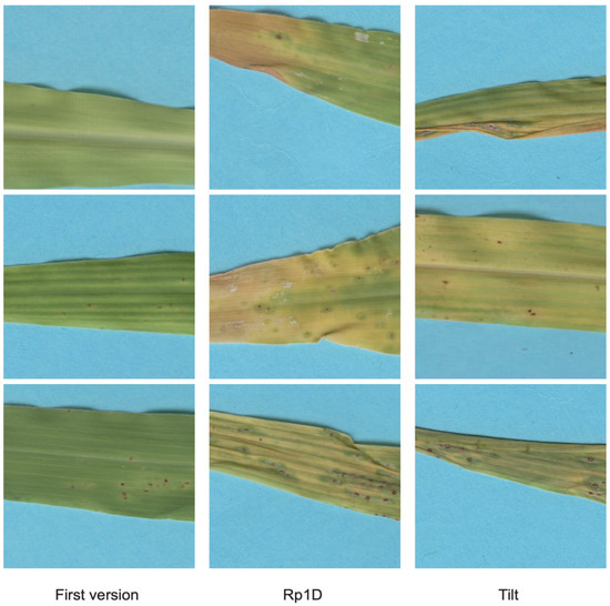
Figure 1.
Comparison of images from the three ISU maize disease datasets, from left to right, first version then Rp1d, and lastly, Tilt.
5.2. Experiment 2—Design Reusability
5.2.1. Text Processing
Table 9 and Table 10 show that in certain instances, such as when the Coronavirus dataset is the target and the ACL IMDB movie reviews dataset is the source, the design does appear to be reusable. Another instance of a design being reusable is seen when Enron is the target and the YouTube comments dataset is the source. Reusability is only achieved when the performance of a deep neural network pipeline design that is being reused is statistically similar to the performance of a deep neural network pipeline design that has been designed from scratch.
From the results, it is clear that there are plenty of instances of design reuse producing exceedingly poor results, meaning that the design is not reusable. In fulfilment of the second objective of this research, the results indicate that designs produced by the SPHH do not appear to be reusable. However, there are certain instances of design reuse that were effective.
It is desirable to have reusable designs, as it means that a new deep neural network pipeline does not need to be designed from scratch every single time the dataset changes, which saves computational cost. In order to adjust the SPHH to produce reusable designs, different datasets can be used at once during design time. Another way to adjust the SPHH for reusability could be to design multiple deep neural network pipelines and subsequently create an ensemble. Ensembles could be more reusable than single deep neural network pipeline designs. Future work will investigate this further.
5.2.2. Image Processing
Table 11 shows that for both image classification and image segmentation, designs do not appear to be reusable, as the performance is not comparable to the performance resulting from a design that was explicitly created for a given dataset. With regard to the second research object, the results again confirm that the SPHH does not produce reusable designs.
5.3. Experiment 3—Automated Design with Transfer Learning
5.3.1. Text Processing
Table 12 and Table 13 show that transfer learning is incredibly effective on the whole; however, the choice of source for transfer learning does seem to have an effect on the efficacy of the transfer learning. In certain instances, such as when using the Yelp dataset as the source of design for the ACL IMDB movie reviews dataset, the use of transfer learning resulted in poorer performance. However, for some datasets, such as when using the SMS Spam dataset as source and the Enron dataset as target, transfer learning resulted in better performance than when no transfer learning was used.
The third objective of this research questioned whether transfer learning would be possible when carrying out automated design of the deep neural network pipeline. The results in Table 12 and Table 13 confirm that while transfer learning is possible and, when done well, even improves performance in certain instances, it cannot be conducted thoughtlessly. The target and source must be carefully considered. Future research will investigate the correlation between the source and target for transfer learning.
5.3.2. Image Processing
The results from Table 15 indicate that transfer learning used in the image processing domain was ineffective for the classification, but it was very effective for the segmentation. For the classification, a decrease in performance was observed when referring back to Table 18 which describes the design choices made. This is not surprising, as the source and target dataset had very different designs created for them, meaning that transfer learning would result in the search being initialized in a sub-optimal location. For image segmentation, the Tilt dataset showed an increase in performance, to which the other dataset (Rp1d) showed similar performance when transfer learning is not used. The image segmentation results can also be explained by referring back to Table 18. which shows that the source and target datasets had very similar designs produced for them.
6. Conclusions
This research has shown that automated design of a deep neural network pipeline using a single-point hyper-heuristic is effective for the image processing and text processing domains. Automating the design of a deep neural network pipeline by means of a SPHH results in pipelines that are competitive with manually derived pipeline designs published in the literature for some of the datasets presented.
The results show that reusing designs created by the SPHH does not provide comparable performance to the results achieved when specifically creating a design for a dataset. The designs are therefore not reusable for either the image processing or text processing domain.
Transfer learning was found to produce results comparable to or better than the results achieved when using the SPHH without transfer learning. Importantly, however, transfer learning was only effective when the correct target and source are chosen. For some target datasets, negative transfer occurs when using certain datasets as the transfer learning source.
Future work will include applying the automated design system to more domains and datasets, as well as looking at how to potentially make designs more reusable. Future work will look at automating the transfer learning process to ensure only positive transfer occurs. Future work should also use automated design to construct a pipeline for unsupervised deep learning techniques instead of deep neural networks, as the state of the literature indicates a steady increase in interest in unsupervised deep-learning techniques. Lastly, future work will include checking the sensitivity of the SPHH to its parameters.
Author Contributions
Conceptualization, M.G. and N.P.; methodology, M.G. and N.P.; formal analysis, M.G. and N.P.; investigation, M.G. and N.P.; data curation, M.G. and N.P.; writing—original draft preparation, M.G. and N.P.; writing—review and editing, M.G. and N.P.; supervision, N.P.; project administration, N.P.; funding acquisition, N.P. All authors have read and agreed to the published version of the manuscript.
Funding
This research was funded by the National Research Foundation of South Africa (Grant Numbers 46712). The opinions expressed and conclusions arrived at are those of the authors and are not necessarily to be attributed to the NRF.
Acknowledgments
The authors would like to thank Katerina Holan for taking the photographs as well as partially annotating the images used in the ISU V1, ISU Rp1d and ISU Tilt datasets [47].
Conflicts of Interest
The authors declare no conflict of interest.
Abbreviations
The following abbreviations are used in this manuscript:
| DNN | Deep Neural Network. |
| RNN | Recurrent Neural Network. |
| CNN | Convolutional Neural Network. |
| LSTM | Long Short-Term Memory. |
| SPHH | Selection Perturbative Hyper-Heuristic. |
Appendix A. Deep Neural Network Pipeline
Appendix A.1. Preprocessing
This section describes the options for each of the processes that make up the deep learning pipeline. Different preprocessing is needed for image processing and text processing.
Appendix A.1.1. Image Processing
Preprocessing options include:
- Mean normalization [11]: This technique will first calculate the mean pixel value across the entire dataset, then preprocess each image in the dataset by subtracting the mean pixel value from each pixel in the image. In the case of images that have multiple channels (i.e., RGB or HSV) the mean pixel value can be calculated per channel.
- Gaussian blur [61]: This technique is commonly used to remove unwanted noise. This filtering technique will consider a single pixel at a time, then set the value of the pixel to be the weighted average of the pixels surrounding it. The number of pixels considered is determined by the kernel size of the filter, and the weighting of pixel values is given by a Gaussian distribution. The resulting output of a Gaussian blur filter is an image that is smoother than the original.
- Moving an image from RGB to HSV colour space [61]: This technique is commonly used, as HSV allows for separation of the colour itself from the intensity of the colour, while RGB does not. Additionally, for certain datasets, the RGB representation can be found to be noisier than the HSV representation.
- Segmenting an image using K-means clustering [61]: This technique is most commonly used to isolate important foreground information from meaningless background information. K-means clustering will be performed with a cluster size of 2. Once the pixels belonging to the background are identified, they will have their pixel value set to be black.
- Enhance contrast [62]: This technique can be applied to both greyscale and colour images. In both cases, the pixel values of the images will be changed in order to enhance image intensity. Contrast enhancement is carried out in an attempt to make features in the image that could be important to the classifier stand out more.
Appendix A.1.2. Text Processing
This section describes the options for each of the processes that make up the deep learning pipeline for text processing. Preprocessing options include:
- Spelling correction: Correcting the spelling of words in the text according to a dictionary that matches the language of the text.
- Lemmatization: Converting similar words to a single word that encompasses the same concept. The difference between stemming and lemmatization is that stemming converts similar words to their stem and lemmatization converts words to their lemma. The lemma of a word takes the morphological origin of a word into account.
- Stemming: Transforming words to their specific stem by cutting off the extra characters from the end of the word. For example, the words “games”, “gamer” and “gamest” will all be transformed to the single stem “game”.
- Removal of stop words: Removing words that occur very often in texts but can be seen as neutral in terms of the meaning they add to a text. Stop words can include words such as: “the”, “a”, “was”, “on” and so forth.
- Removal of hash tags: Converting hashtags into normal words. The reason why this is done is due to the leading pound sign ie “#weekend”. Hashtags will be seen as unique words.
- Removal of URLs and URI-type strings: Removing these strings where an example of a URL is ‘http://example.com’ and an example of a URI is ‘urn:oasis:names:specification: docbook:dtd:xml:4.1.2’.
- Removal of punctuation: Removing punctuation is often carried out to combine multiple sentences into a single sentence.
- Conversion of all text to lowercase: Converting all uppercase letters to their lowercase equivalent is carried out to decrease variance in the dataset.
Appendix A.2. Data Augmentation
This process in the pipeline is specific to image processing and is not needed for text processing. Research has shown that data augmentation techniques can result in better performance of subsequent classification [63] and segmentation [64] of deep neural network techniques. Methods for data augmentation include:
- Flipping of the image [10].
- Rotation of an image [10].
- Cropping an image to be smaller than the original [10].
- Changing the position of the centre point of the image [10].
- Changing the colour space of an image [10].
- Adding noise to an image [65].
- Sharpening the image [65].
Appendix A.3. Feature Engineering
Feature engineering is specific to text processing. Techniques generally used include:
- One hot encoding creates a vector representation for each word within the text. The vector representation will have elements that are either zero or one only, and each position in the vector corresponds to a position within the text. If the word for which we are creating the vector appears in a specific position in the text, the same position in the vector will have a one. Conversely, if the word for which we are creating the vector does not appear in a specific position within the text, the same position in the vector will have a 0. A vector representation is created for each and every word within the text, including punctuation, if it was not removed during preprocessing. The resulting collection of vectors will be the feature representation.
- Term frequency—inverse document frequency (TF-IDF) [66] calculates how frequently a word occurs in a single textual instance (term frequency) and then multiplies that value by the inverse of how frequently that word occurs across multiple texts (inverse document frequency).
- Word2Vec (CBOW model) [67] uses cosine similarity to group similar words together. A word vector (the context) will represent the words that are most similar to the word. Each unique word in the text as a whole will have a word vector generated for it. Word2Vec makes use of a two-layer neural network to generate the word vectors and has two distinct variations in architecture, the first being the continuous bag of words (CBOW) architecture and the second the Skip-gram architecture. In the CBOW architecture, the neural network is given a specific context (collection of words) from the text as a whole and attempts to predict the single word that would fit that context. If the prediction is incorrect, the vector for the single word is adjusted accordingly.
- Word2Vec (Skip-gram model) [67] uses cosine similarity to group similar words together. A word vector (the context) will represent the words that are most similar to the word. Each unique word in the text as a whole will have a word vector generated for it. Word2Vec makes use of a two-layer neural network to generate the word vectors, and has two distinct variations in architecture, the first being the continuous bag of words (CBOW) architecture and the second the Skip-gram architecture. In the Skip-gram architecture, the neural network is given a single word and attempts to predict the context (collection of words) within the text as a whole that the single word would occur in. If the prediction is incorrect, the vector for the single word is adjusted accordingly.
- GloVe [68] makes use of unsupervised learning and, like TF-IDF, makes use of word frequency vectors for each word. The GloVe technique will then calculate the dot product of two word vectors and compare it to the log of the amount of times the two words occur near one another. The two word vectors are then adjusted based on how different the dot product is from the log result. The concept of how “near” two words are to one another is controlled by a hyper-parameter.
- FastText [69] extends the Word2Vec model by encoding the individual words into their n-gram representation before training the neural network. An n-gram is created by sampling a number of contiguous characters from a word. The number of characters to be sampled is greater than one and smaller than or equal to n. The use of n-grams for the representation allows for longer words to be broken up into their prefixes and suffixes and shorter words to be better explicated.
Appendix A.4. Neural Network Architecture Selection
This section describes the process of the pipeline involving selection of the neural network for the problem at hand. The section provides an overview of the networks generally used for image processing and text processing based on a review of previous work in the field.
Neural networks that have been used for text processing include convolutional neural networks (CNNs), deep neural networks (DNNs), recurrent neural networks (RNN) and long-short-term memory (LSTM).
Neural networks used for segmentation for image processing include: Poly YOLO [70], U-Net [71] and Mask R-CNN [72]. Neural networks used for classification for image processing include: Xception [73], VGG16 and VGG19 [74], ResNet50, ResNet101 and ResNet152 [75], ResNet50V2, ResNet101V2 and ResNet152V2 [76], InceptionV3 [77], InceptionResNetV2 [78], MobileNet [79], MobileNetV2 [80], DenseNet121, DenseNet169 and DenseNet201 [81].
Appendix A.5. Hyperparameter Tuning
For both image processing and text processing, each of the deep neural network architectures have the following hyper-parameters that will also be tuned as part of the automated design process:
- Optimizer algorithm, which can take one of the following values: Stochastic gradient descent, RMSProp, Adam, Adadelta, Adagrad, Adamax, NAdam and Ftrl.
- Loss function, which can take one of the following values: Binary crossentropy, Poisson, Mean squared error, Mean absolute error, Mean absolute percentage error, Mean squared logarithmic error, Cosine similarity, Squared hinge, Categorical hinge and hinge.
- Activation function, which can take one of the following values: ReLU, Sigmoid, Softmax, Softplus, Tanh, SeLU, eLU, Exponential and softsign.
- Kernel initializer, which can take one of the following values: Random normal, Random uniform, Truncated normal, Zeros, Ones, Glorot normal, Glorot uniform and constant.
- Bias initializer, which can take the same values as specified for the above kernel initializer.
Appendix B. Selection Hyper-Heuristic for Automated Design (SPHH)—Heuristic Selection
The hyper-heuristic consists of two components, the heuristic selector and move acceptor. This section describes the choice function [7] used for heuristic selection. The choice function is used to rank each perturbative heuristic using the following formula:
The low-level perturbative heuristic is represented as . represents ’s performance over the previous n times that it was applied. is the change in the deep neural network pipeline’s testing accuracy from the last invocation. is the time difference in seconds between the last application of .
The second constituent part of f is , which represents a comparison between and all other low-level perturbative heuristics in the heuristic space , in the instances where and were applied in succession. is now the difference in the deep neural network pipeline’s testing accuracy from one successive application of and to the next. is the time difference in seconds between the last successive invocation of and .
The last part is the time in CPU seconds since was last applied.
The equation f has three extra parameters: , and . Both and are used to increase or decrease the influence that hi’s recent performance has. The parameter is used to increase diversity.
Appendix C. Experimental Setup—Datasets
Appendix C.1. Text Processing Datasets
Appendix C.1.1. Sentiment Analysis
- ACL IMDB movie reviews dataset [28]. This dataset is made up of movie reviews made on the IMDB website. Importantly, only highly polarized reviews—reviews with less than or equal to 4 stars or reviews with more than or equal to 7 stars—are included. This dataset comprises of 50,000 instances, where 25,000 have positive sentiment and 25,000 have negative sentiment.
- Amazon product reviews dataset [29]. This dataset is made up of user reviews on the Amazon website. The following categories from the “unprocessed.tar” folder were selected: apparel, automotive, baby, beauty, books, camera_&_photo, cell_phones_&_service, computer_&_video_games, dvd, electronics, gourmet_food, grocery, health_&_personal_care, jewelry_&_watches, kitchen_&_housewares, magazines, music, musical_instruments, office_products, outdoor_living, software, sports_&_outdoors. tools_&_hardware, toys_&_ games and video. This resulted in a total of 38,548 instances. Of those instances, 21,972 had positive sentiment and 16,576 had negative sentiment.
- Coronavirus tweets dataset [30]. This dataset is made up of tweets gathered from Twitter from March 2020 onwards and contains tweets relating to COVID-19. The full dataset is continually growing, as the COVID-19 pandemic is an ongoing event. For this reason, only a subset of the full dataset was used, namely the dataset file named “coronavirus_tweets_01.csv”. This contains a total of 831,328 instances, in which the sentiment score ranges between to 1.0.
- Sentiment 140 dataset [31]. This dataset is made up of tweets gathered from Twitter, in which the emoticons within the tweets decided the sentiment of the tweet. This dataset contains a total of 1.6 million instances, in which 800,000 of those instances had a positive sentiment and 800,000 of those instances had a negative sentiment.
- Yelp reviews dataset [32], this dataset is made up of user reviews for businesses, as recorded on the website Yelp. A total of 342,858 instances were used from the Yelp academic reviews dataset, where the stars attribute given for each instance was used to determine sentiment. The stars attribute is an integer within the range 1 to 5, inclusive.
Appendix C.1.2. Spam Detection
- Enron email dataset [39], this dataset contains a subset of the total Enron dataset, which is made up of leaked emails from employees that worked at Enron in 2002. This dataset specifically focuses on six users: farmer-d, kaminski-v, kitchen-l, williams-w3, beck-s, and lokay-m. The total amount of instances in this dataset is 33,716, where 17,171 of these emails are spam and 16,545 of these emails are ham.
- SMS spam dataset [40], this dataset consists of a collection of short messaging system (SMS) messages. This dataset has a total of 5575 instances where 4850 of those instances are ham and 725 of those instances are spam.
- Spam assassin dataset [41], this dataset was created from a selection of email messages made available publicly for the express purpose of testing spam filtering systems for email clients. This dataset has a total of 6047 instances, where 1897 of those instances are spam and 4150 of those are ham.
- YouTube comments spam dataset [42]. This dataset contains comments from five YouTube videos. The total amount of instances in this dataset comes to 1956, with 951 instances being ham and 1005 instances being spam.
Appendix C.2. Image Processing Datasets
Appendix C.2.1. Image Classification
- Oral lesion dataset [48]. This dataset consists of 352 colour photos of patients’ mouths that show some kind of oral lesion, in which 165 of the images are classified as benign lesions and 187 of the images are classified as malignant lesions. The Oral Lesion Dataset also contains 2622 augmented images, where 1156 of the augmented images are classified as benign and 1115 of the augmented images are classified as malignant.
- University of Pretoria (UP) oral lesion images dataset [49]. This dataset consists of colour photos taken of patients’ mouths that display both benign and malignant lesions. The photos were provided by the Periodontics and Oral Medicine department at the University of Pretoria. The dataset consists of 69 images, where 60 of the images were classified as benign and 9 of the images were classified as malignant.
Appendix C.2.2. Image Segmentation
- Iowa State University (ISU) maize disease dataset—first version [47], this dataset was created from maize plants grown in a greenhouse at Iowa State University. The maize plants were inoculated by spraying the leaves with common rust urediniospores. At different stages of infection, maize leaves were removed and scanned on a flatbed scanner at 1200 DPI. This dataset consists of 1040 images in total.
- Iowa State University (ISU) maize disease dataset—Rp1D inoculation method. This dataset was created from maize plants grown in a greenhouse at Iowa State University. The maize plants were inoculated by means of the Rp1D method. At different stages of infection, maize leaves were removed and scanned on a flatbed scanner at 1200 DPI. This dataset consists of 167 images in total.
- Iowa State University (ISU) maize disease dataset—Tilt inoculation method. This dataset was created from maize plants grown in a greenhouse at Iowa State University. The maize plants were inoculated by means of the Tilt method. At different stages of infection, maize leaves were removed and scanned on a flatbed scanner at 1200 DPI. This dataset consists of 1114 images in total.
References
- Alom, M.Z.; Taha, T.M.; Yakopcic, C.; Westberg, S.; Sidike, P.; Nasrin, M.S.; Esesn, B.C.V.; Awwal, A.A.S.; Asari, V.K. The History Began from AlexNet: A Comprehensive Survey on Deep Learning Approaches. arXiv 2018, arXiv:1803.01164. [Google Scholar]
- Liu, W.; Wang, Z.; Liu, X.; Zeng, N.; Liu, Y.; Alsaadi, F.E. A survey of deep neural network architectures and their applications. Neurocomputing 2017, 234, 11–26. [Google Scholar] [CrossRef]
- Hutter, F.; Kotthoff, L.; Vanschoren, J. Automated Machine Learning: Methods, Systems, Challenges; Springer Nature: Berlin/Heidelberg, Germany, 2019; p. 9. [Google Scholar]
- Pham, H.; Guan, M.; Zoph, B.; Le, Q.; Dean, J. Efficient neural architecture search via parameters sharing. In Proceedings of the International Conference on Machine Learning, PMLR, Stockholm, Sweden, 10–15 July 2018; pp. 4095–4104. [Google Scholar]
- Romano, J.D.; Le, T.T.; Fu, W.; Moore, J.H. TPOT-NN: Augmenting tree-based automated machine learning with neural network estimators. Genet. Program. Evolvable Mach. 2021, 22, 207–227. [Google Scholar] [CrossRef]
- Pillay, N.; Qu, R. Automated Design of Machine Learning and Search Algorithms; Springer: Berlin/Heidelberg, Germany, 2021. [Google Scholar]
- Pillay, N.; Qu, R. Hyper-Heuristics: Theory and Applications; Springer: Berlin/Heidelberg, Germany, 2018. [Google Scholar]
- Gerber, M. Automated Design of the Deep Neural Network Pipeline. 2021. Available online: https://www.cs.up.ac.za/cs/nicog/ThPane.htm (accessed on 1 April 2020).
- Minaee, S.; Kalchbrenner, N.; Cambria, E.; Nikzad, N.; Chenaghlu, M.; Gao, J. Deep Learning–based Text Classification: A Comprehensive Review. ACM Comput. Surv. CSUR 2021, 54, 62. [Google Scholar] [CrossRef]
- Shorten, C.; Khoshgoftaar, T.M. A survey on image data augmentation for deep learning. J. Big Data 2019, 6, 60. [Google Scholar] [CrossRef]
- Pal, K.K.; Sudeep, K.S. Preprocessing for image classification by convolutional neural networks. In Proceedings of the 2016 IEEE International Conference on Recent Trends in Electronics, Information Communication Technology (RTEICT), Bangalore, India, 20–21 May 2016; pp. 1778–1781. [Google Scholar] [CrossRef]
- Uysal, A.K.; Gunal, S. The impact of preprocessing on text classification. Inf. Process. Manag. 2014, 50, 104–112. [Google Scholar] [CrossRef]
- Casado-García, Á.; Domínguez, C.; García-Domínguez, M.; Heras, J.; Inés, A.; Mata, E.; Pascual, V. CLoDSA: A tool for augmentation in classification, localization, detection, semantic segmentation and instance segmentation tasks. BMC Bioinform. 2019, 20, 323. [Google Scholar] [CrossRef]
- Madasu, A.; Elango, S. Efficient feature selection techniques for sentiment analysis. Multimed. Tools Appl. 2020, 79, 6313–6335. [Google Scholar] [CrossRef]
- Abidemi, T.I.F.; Toyin, T.N. Feature extraction for SMS spam detection. Int. J. Adv. Sci. Res. 2020, 5, 21–25. [Google Scholar]
- Hassan, M.A.; Mtetwa, N. Feature extraction and classification of spam emails. In Proceedings of the 2018 5th International Conference on Soft Computing & Machine Intelligence (ISCMI), IEEE, Nairobi, Kenya, 21–22 November 2018; pp. 93–98. [Google Scholar]
- Marani, R.; Milella, A.; Petitti, A.; Reina, G. Deep neural networks for grape bunch segmentation in natural images from a consumer-grade camera. Precis. Agric. 2021, 22, 387–413. [Google Scholar] [CrossRef]
- Too, E.C.; Yujian, L.; Njuki, S.; Yingchun, L. A comparative study of fine-tuning deep learning models for plant disease identification. Comput. Electron. Agric. 2019, 161, 272–279. [Google Scholar] [CrossRef]
- Kassani, S.H.; Kassani, P.H. A comparative study of deep learning architectures on melanoma detection. Tissue Cell 2019, 58, 76–83. [Google Scholar] [CrossRef]
- Dang, N.C.; Moreno-García, M.N.; De la Prieta, F. Sentiment analysis based on deep learning: A comparative study. Electronics 2020, 9, 483. [Google Scholar] [CrossRef]
- Hajek, P.; Barushka, A.; Munk, M. Fake consumer review detection using deep neural networks integrating word embeddings and emotion mining. Neural Comput. Appl. 2020, 32, 17259–17274. [Google Scholar] [CrossRef]
- Whitley, D.; Watson, J.P. Complexity theory and the no free lunch theorem. In Search Methodologies; Springer: Berlin/Heidelberg, Germany, 2005; pp. 317–339. [Google Scholar]
- Stanley, K.O.; Clune, J.; Lehman, J.; Miikkulainen, R. Designing neural networks through neuroevolution. Nat. Mach. Intell. 2019, 1, 24–35. [Google Scholar] [CrossRef]
- Elsken, T.; Metzen, J.H.; Hutter, F. Neural architecture search: A survey. J. Mach. Learn. Res. 2019, 20, 1997–2017. [Google Scholar]
- He, X.; Zhao, K.; Chu, X. AutoML: A Survey of the State-of-the-Art. Knowl.-Based Syst. 2021, 212, 106622. [Google Scholar] [CrossRef]
- Weiss, K.; Khoshgoftaar, T.M.; Wang, D. A survey of transfer learning. J. Big Data 2016, 3, 9. [Google Scholar] [CrossRef]
- Wong, C.; Houlsby, N.; Lu, Y.; Gesmundo, A. Transfer learning with neural automl. arXiv 2018, arXiv:1803.02780. [Google Scholar]
- Maas, A.L.; Daly, R.E.; Pham, P.T.; Huang, D.; Ng, A.Y.; Potts, C. Learning Word Vectors for Sentiment Analysis. In Proceedings of the 49th Annual Meeting of the Association for Computational Linguistics: Human Language Technologies, Portland, OR, USA, 19–24 June 2011; Association for Computational Linguistics: Portland, OR, USA, 2011; pp. 142–150. [Google Scholar]
- Blitzer, J.; Dredze, M.; Pereira, F. Biographies, bollywood, boom-boxes and blenders: Domain adaptation for sentiment classification. In Proceedings of the 45th Annual Meeting of the Association of Computational Linguistics, Prague, Czech Republic, 25–27 June 2007; pp. 440–447. [Google Scholar]
- Lamsal, R. Design and analysis of a large-scale COVID-19 tweets dataset. Appl. Intell. 2020, 51, 2790–2804. [Google Scholar] [CrossRef]
- Go, A.; Bhayani, R.; Huang, L. Twitter sentiment classification using distant supervision. CS224N Proj. Rep. Stanf. 2009, 1, 2009. [Google Scholar]
- Yelp Inc. Yelp Reviews Dataset. 2014. Available online: https://www.yelp.com/dataset/download (accessed on 1 November 2020).
- Gogineni, S.; Pimpalshende, A. Predicting IMDB Movie Rating Using Deep Learning. In Proceedings of the 2020 5th International Conference on Communication and Electronics Systems (ICCES), Coimbatore, India, 10–12 June 2020; pp. 1139–1144. [Google Scholar] [CrossRef]
- Widayat, W.; Adji, T.B.; Widyawan. The Effect of Embedding Dimension Reduction on Increasing LSTM Performance for Sentiment Analysis. In Proceedings of the 2018 International Seminar on Research of Information Technology and Intelligent Systems (ISRITI), Yogyakarta, Indonesia, 21–22 November 2018; pp. 287–292. [Google Scholar] [CrossRef]
- Das, S.; Kolya, A.K. Predicting the pandemic: Sentiment evaluation and predictive analysis from large-scale tweets on Covid-19 by deep convolutional neural network. Evol. Intell. 2021, 15, 1913–1934. [Google Scholar] [CrossRef]
- Srinivas, A.C.M.V.; Satyanarayana, C.; Divakar, C.; Sirisha, K.P. Sentiment Analysis using Neural Network and LSTM. In Proceedings of the IOP Conference Series: Materials Science and Engineering, Kakinada, India, 28–29 December 2021; Volume 1074, p. 012007. [Google Scholar]
- Alamoudi, E.S.; Alghamdi, N.S. Sentiment classification and aspect-based sentiment analysis on yelp reviews using deep learning and word embeddings. J. Decis. Syst. 2021, 30, 259–281. [Google Scholar] [CrossRef]
- Ferrara, E. The history of digital spam. Commun. ACM 2019, 62, 82–91. [Google Scholar] [CrossRef]
- Metsis, V.; Androutsopoulos, I.; Paliouras, G. Spam filtering with naive bayes-which naive bayes? In Proceedings of the Third Conference on Email and Anti-Spam—CEAS, Mountain View, CA, USA, 27–28 July 2006; Volume 17, pp. 28–69. [Google Scholar]
- Almeida, A.T.; Hidalgo, J.M.G. SMS Spam Collection. 2018. Available online: http://www.dt.fee.unicamp.br/~tiago/smsspamcollection/ (accessed on 1 November 2020).
- Apache Software Foundation Spam Assassin Public Corpus. 2015. Available online: https://spamassassin.apache.org/ (accessed on 1 November 2020).
- Alberto, T.C.; Lochter, J.V.; Almeida, T.A. Tubespam: Comment spam filtering on youtube. In Proceedings of the 2015 IEEE 14th International Conference on Machine Learning and Applications (ICMLA), Miami, FL, USA, 9–11 December 2015; pp. 138–143. [Google Scholar]
- Barushka, A.; Hajek, P. Spam filtering using integrated distribution-based balancing approach and regularized deep neural networks. Appl. Intell. 2018, 48, 3538–3556. [Google Scholar] [CrossRef]
- Taheri, R.; Javidan, R. Spam filtering in SMS using recurrent neural networks. In Proceedings of the 2017 Artificial Intelligence and Signal Processing Conference (AISP), Shiraz, Iran, 25–27 October 2017; pp. 331–336. [Google Scholar]
- Lee, M.H. A Study of Efficiency Information Filtering System using One-Hot Long Short-Term Memory. Int. J. Adv. Cult. Technol. 2017, 5, 83–89. [Google Scholar]
- Chetty, G.; Bui, H.; White, M. Deep learning based spam detection system. In Proceedings of the 2019 International Conference on Machine Learning and Data Engineering (iCMLDE), IEEE, Taipei, Taiwan, 2–4 December 2019; pp. 91–96. [Google Scholar]
- Pillay, N.; Gerber, M.; Holan, K.; Whitham, S.A.; Berger, D.K. Quantifying the Severity of Common Rust in Maize Using Mask R-CNN. In Proceedings of the Artificial Intelligence and Soft Computing: 20th International Conference, ICAISC 2021, Virtual Event, 21–23 June 2021. Proceedings, Part I. [Google Scholar] [CrossRef]
- Chandrashekar, H.S.; Geetha Kiran, A.; S, M.; Dinesh, M.; Nanditha, B. Oral Images Dataset. 2021. Available online: https://data.mendeley.com/datasets/mhjyrn35p4/2 (accessed on 1 November 2020).
- Gerber, M.; Pillay, N.; Khammissa, R. A Comparative Study of Supervised and Unsupervised Neural Networks for Oral Lesion Detection. In Proceedings of the 2021 IEEE Symposium Series on Computational Intelligence, Orlando, FL, USA, 5–7 December 2021. [Google Scholar]
- Misir, M.; Verbeeck, K.; De Causmaecker, P.; Berghe, G.V. Hyper-heuristics with a dynamic heuristic set for the home care scheduling problem. In Proceedings of the IEEE Congress on Evolutionary Computation, Barcelona, Spain, 18–23 July 2010; pp. 1–8. [Google Scholar]
- Sachan, D.S.; Zaheer, M.; Salakhutdinov, R. Revisiting LSTM Networks for Semi-Supervised Text Classification via Mixed Objective Function. Proc. AAAI Conf. Artif. Intell. 2019, 33, 6940–6948. [Google Scholar] [CrossRef]
- Xiao, L.; Zhang, H.; Chen, W.; Wang, Y.; Jin, Y. Transformable Convolutional Neural Network for Text Classification. In Proceedings of the Twenty-Seventh International Joint Conference on Artificial Intelligence—IJCAI, Stockholm, Sweden, 13–19 July 2018; pp. 4496–4502. [Google Scholar]
- Başarslan, M.S.; Kayaalp, F. Sentiment Analysis on Social Media Reviews Datasets with Deep Learning Approach. Sak. Univ. J. Comput. Inf. Sci. 2021, 4, 35–49. [Google Scholar] [CrossRef]
- Lai, K.P.; Lam, W.; Ho, J.C. Domain-Aware Recurrent Neural Network for Cross-Domain Sentiment Classification. In Proceedings of the 3rd International Conference on Data Science and Information Technology, Xiamen, China, 24–26 July 2020; pp. 181–185. [Google Scholar]
- Chakraborty, K.; Bhatia, S.; Bhattacharyya, S.; Platos, J.; Bag, R.; Hassanien, A.E. Sentiment Analysis of COVID-19 tweets by Deep Learning Classifiers—A study to show how popularity is affecting accuracy in social media. Appl. Soft Comput. 2020, 97, 106754. [Google Scholar] [CrossRef] [PubMed]
- Hankamer, D.; Liedtka, D. Twitter Sentiment Analysis with Emojis. 2018. Available online: http://davidliedtka.com/docs/cs224u.pdf (accessed on 1 January 2021).
- Hamdi, E.; Rady, S.; Aref, M. A Deep Learning Architecture with Word Embeddings to Classify Sentiment in Twitter. In Proceedings of the International Conference on Advanced Intelligent Systems and Informatics, Cairo, Egypt, 19–21 October 2020; Springer: Berlin/Heidelberg, Germany, 2020; pp. 115–125. [Google Scholar]
- Srinivasan, S.; Ravi, V.; Alazab, M.; Ketha, S.; Ala’M, A.Z.; Padannayil, S.K. Spam Emails Detection Based on Distributed Word Embedding with Deep Learning. In Machine Intelligence and Big Data Analytics for Cybersecurity Applications; Springer: Berlin/Heidelberg, Germany, 2021; pp. 161–189. [Google Scholar]
- Roy, P.K.; Singh, J.P.; Banerjee, S. Deep learning to filter SMS Spam. Future Gener. Comput. Syst. 2020, 102, 524–533. [Google Scholar] [CrossRef]
- Uysal, A.K. Feature selection for comment spam filtering on YouTube. Data Sci. Appl. 2018, 1, 4–8. [Google Scholar]
- Sharma, P.; Hans, P.; Gupta, S.C. Classification Of Plant Leaf Diseases Using Machine Learning And Image Preprocessing Techniques. In Proceedings of the 2020 10th International Conference on Cloud Computing, Data Science Engineering (Confluence), Noida, India, 29–31 January 2020; pp. 480–484. [Google Scholar] [CrossRef]
- Rodríguez-Cristerna, A.; Guerrero-Cedillo, C.P.; Donati-Olvera, G.A.; Gómez-Flores, W.; Pereira, W.C.A. Study of the impact of image preprocessing approaches on the segmentation and classification of breast lesions on ultrasound. In Proceedings of the 2017 14th International Conference on Electrical Engineering, Computing Science and Automatic Control (CCE), Mexico City, Mexico, 20–22 October 2017; pp. 1–4. [Google Scholar] [CrossRef]
- Hussain, Z.; Gimenez, F.; Yi, D.; Rubin, D. Differential data augmentation techniques for medical imaging classification tasks. AMIA Annu. Symp. Proc. 2018, 2017, 979–984. [Google Scholar]
- O’Gara, S.; McGuinness, K. Comparing data augmentation strategies for deep image classification. In Proceedings of the Irish Machine Vision and Image Processing Conference (IMVIP), Dublin, Ireland, 28–30 August 2019. [Google Scholar]
- Zhang, C.; Zhou, P.; Li, C.; Liu, L. A convolutional neural network for leaves recognition using data augmentation. In Proceedings of the 2015 IEEE International Conference on Computer and Information Technology; Ubiquitous Computing and Communications; Dependable, Autonomic and Secure Computing; Pervasive Intelligence and Computing, Liverpool, UK, 26–28 October 2015; pp. 2143–2150. [Google Scholar]
- Sammut, C.; Webb, G.I. (Eds.) TF–IDF. In Encyclopedia of Machine Learning; Springer: Boston, MA, USA, 2010; pp. 986–987. [Google Scholar] [CrossRef]
- Mikolov, T.; Chen, K.; Corrado, G.; Dean, J. Efficient estimation of word representations in vector space. arXiv 2013, arXiv:1301.3781. [Google Scholar]
- Pennington, J.; Socher, R.; Manning, C.D. Glove: Global vectors for word representation. In Proceedings of the 2014 Conference on Empirical Methods in Natural Language Processing (EMNLP), Doha, Qatar, 25–29 October 2014; pp. 1532–1543. [Google Scholar]
- Bojanowski, P.; Grave, E.; Joulin, A.; Mikolov, T. Enriching word vectors with subword information. Trans. Assoc. Comput. Linguist. 2017, 5, 135–146. [Google Scholar] [CrossRef]
- Hurtik, P.; Molek, V.; Hula, J.; Vajgl, M.; Vlasanek, P.; Nejezchleba, T. Poly-YOLO: Higher speed, more precise detection and instance segmentation for YOLOv3. arXiv 2020, arXiv:2005.13243. [Google Scholar] [CrossRef]
- Ronneberger, O.; Fischer, P.; Brox, T. U-net: Convolutional networks for biomedical image segmentation. In Proceedings of the International Conference on Medical Image Computing and Computer-Assisted Intervention, Munich, Germany, 5–9 October 2015; Springer: Berlin/Heidelberg, Germany, 2015; pp. 234–241. [Google Scholar]
- He, K.; Gkioxari, G.; Dollár, P.; Girshick, R. Mask r-cnn. In Proceedings of the IEEE International Conference on Computer Vision, Venice, Italy, 22–29 October 2017; pp. 2961–2969. [Google Scholar]
- Chollet, F. Xception: Deep learning with depthwise separable convolutions. In Proceedings of the IEEE Conference on Computer Vision and Pattern Recognition, Honolulu, HI, USA, 21–26 July 2017; pp. 1251–1258. [Google Scholar]
- Simonyan, K.; Zisserman, A. Very deep convolutional networks for large-scale image recognition. arXiv 2014, arXiv:1409.1556. [Google Scholar]
- He, K.; Zhang, X.; Ren, S.; Sun, J. Deep residual learning for image recognition. In Proceedings of the IEEE Conference on Computer Vision and Pattern Recognition, Las Vegas, NV, USA, 27–30 June 2016; pp. 770–778. [Google Scholar]
- He, K.; Zhang, X.; Ren, S.; Sun, J. Identity mappings in deep residual networks. In Proceedings of the European Conference on Computer Vision, Amsterdam, The Netherlands, 11–14 October 2016; Springer: Berlin/Heidelberg, Germany, 2016; pp. 630–645. [Google Scholar]
- Szegedy, C.; Vanhoucke, V.; Ioffe, S.; Shlens, J.; Wojna, Z. Rethinking the inception architecture for computer vision. In Proceedings of the IEEE Conference on Computer Vision and Pattern Recognition, Las Vegas, NV, USA, 27–30 June 2016; pp. 2818–2826. [Google Scholar]
- Szegedy, C.; Ioffe, S.; Vanhoucke, V.; Alemi, A.A. Inception-v4, inception-resnet and the impact of residual connections on learning. In Proceedings of the Thirty-First AAAI Conference on Artificial Intelligence, San Francisco, CA, USA, 4–9 February 2017. [Google Scholar]
- Howard, A.G.; Zhu, M.; Chen, B.; Kalenichenko, D.; Wang, W.; Weyand, T.; Andreetto, M.; Adam, H. Mobilenets: Efficient convolutional neural networks for mobile vision applications. arXiv 2017, arXiv:1704.04861. [Google Scholar]
- Sandler, M.; Howard, A.; Zhu, M.; Zhmoginov, A.; Chen, L.C. Mobilenetv2: Inverted residuals and linear bottlenecks. In Proceedings of the IEEE Conference on Computer Vision and Pattern Recognition, Salt Lake City, UT, USA, 18–23 June 2018; pp. 4510–4520. [Google Scholar]
- Huang, G.; Liu, Z.; Van Der Maaten, L.; Weinberger, K.Q. Densely connected convolutional networks. In Proceedings of the IEEE Conference on Computer Vision and Pattern Recognition, Honolulu, HI, USA, 21–26 July 2017; pp. 4700–4708. [Google Scholar]

Publisher’s Note: MDPI stays neutral with regard to jurisdictional claims in published maps and institutional affiliations. |
© 2022 by the authors. Licensee MDPI, Basel, Switzerland. This article is an open access article distributed under the terms and conditions of the Creative Commons Attribution (CC BY) license (https://creativecommons.org/licenses/by/4.0/).