Fuzzy Neural Network Dynamic Inverse Control Strategy for Quadrotor UAV Based on Atmospheric Turbulence

Abstract

Quadrotor UAV is vulnerable to external interference, which affects search and rescue. In this paper, a fuzzy neural network dynamic inverse controller (FNN-DIC) is designed to eliminate the instability of the attitude angle caused by atmospheric turbulence. Considering the complexity of atmospheric turbulence, the component model of atmospheric turbulence is obtained firstly based on the Dryden model, using Gaussian white noise as a random input signal and a designed shaping filter. Combined with the Newton-Euler equation, a nonlinear dynamic model for the quadrotor UAV with atmospheric disturbance is established. While the traditional nonlinear dynamic inverse cancels the nonlinearity of the controlled object, it relies on precise mathematical models. The fuzzy neural network can adaptively compensate for the inaccurate part of the model and the inverse error of the model caused by the external disturbance, and the stability of the control system is strictly proved by using the Lyapunov function. The experiments are carried out on the simulation platform, and the results show that the FNN method can ensure that the quadrotor UAV can still fly smoothly against strong disturbances, and that robustness of the system is significantly improved.

1. Introduction

The quadrotor UAV can adjust the attitude arbitrarily and has the ability to move at high speed and turn quickly [1,2]. Compared with fixed-wing UAVs, it has obvious advantages in maneuverability and flexibility, which makes it much more suitable for performing high-risk tasks in confined spaces without humans [3,4]. When drones spray pesticides over farms or deliver express delivery in human communities, the design of the controllers is mainly determined by the load problem [5,6,7]. If the search and the rescue work is carried out over a canyon or sea level, not only the harsh environment but also strong winds and atmospheric turbulence should be considered [8,9]. Generally speaking, the turbulent lies in the stern of a ship, which is generated by the heat transfer, wind shear and other reasons [10]. The randomness of atmospheric turbulence is strong, which seriously affects the flight effect of unmanned aerial vehicles. Due to the highly nonlinear and strong coupling of attitudes, external airflow interference during flight [11], the perturbation of aerodynamic parameters for the model, the accurate modeling for quadrotor UAV is considerably difficulty [12]. Under the strong external disturbance, the UAV cannot maintain the desired attitude, which often leads to the failure of the mission. This requires its control system to have strong robustness and anti-interference ability [13].

Linear control is one of the commonly used control methods for quadrotor UAV flight systems. Since the aircraft itself is a nonlinear system, the linearization method can used to obtain an approximate model, and thus reducing the coupling among attitudes. For example, the linearization methods of PID and LQR are both commonly used to improve the performance of flight control systems. Kaba improves the PID algorithm for quadrotor UAV to ensure the optimality of the controller by the convexity-based proxy firefly algorithm, and evaluates the performance under different convex combination values [14]. In the presence of wind and other environmental disturbances, LQR and LQR-PI controllers are employed to reduce the deviation of state trajectory. According to the state variables and preference factors of quadrotor aircraft, the weighting matrix can be automatically adjusted [15]. Since the model is not accurate enough and the controller design process is cumbersome, it is difficult to meet the high-quality requirements for quadrotor UAV. Therefore, the nonlinear control method, which can fully consider the nonlinearity of quadrotor UAV, can be utilized to gain better performance. Different from the approximate linearization, the feedback linearization is better method based on accurate model, which turns the nonlinear system into the linear one by the method of controller design. According to the incremental nonlinear dynamic inversion (INDI), a cascade control method is proposed for the attitude loop and position loop. Compared with the nonlinear calculation, the linearization method is used to calculate the effect of thrust vector increment [16]. Furthermore, the sliding mode control [17], the active disturbance rejection control [18] and the fuzzy control [19] are often used as control algorithms for quadrotor UAV. A dynamic surface-active disturbance rejection control strategy is proposed by Zhang, in which a first-order filter is introduced to obtain the derivative of the virtual control and simplifies the control law of the system. Compared with the classical ADRC controller, the advantages and effectiveness of the developed control strategy are given in the simulations [20]. Noordin proposes a self-correcting adaptive PID control method to solve the problem of attitude and position stability of quadrotor UAV against the parameter uncertainty and external disturbance. By employing the sliding mode control as the adaptive mechanism, the retuning gain of the manual controller for the proportional-integral-derivative controller is overcome. In addition, a blur compensator is used to eliminate the chattering phenomenon caused by sliding mode control [21]. Li designs a fuzzy sliding mode controller to deal with the nonlinearity and uncertainty of the quadrotor UAV. This significantly improves the robustness, response speed and adaptive ability of the system, but the ability to cope with strong external disturbances needs to be further improved [22].

During the actual flight, external interference is unavoidable. The environment around the aircraft is complex and unpredictable, and the accuracy of the model is difficult to guarantee [23]. Neural networks have strong self-learning ability and can approximate nonlinear functions with ideal accuracy. Especially for the flight control system with high control precision, the neural network has the ability of better robustness and real-time performance [24]. Nonlinear terms and coupling terms will affect the control effect of quadrotor UAV. Therefore, Muliadi proposes the method of artificial neural network direct inverse control to overcome the limitations of traditional control methods [25]. At present, a hybrid neural network controller is performed by combining other control methods with neural network. In reference [26], a method combining the neural network with fuzzy control is proposed, which is applied to the take-off and landing control for quadrotor UAV, so that it can overcome various external disturbances and maintain stability. Wai designed an online adaptive neural network controller with different learning rates to ensure the control stability with a reliable anti-interference ability. According to all the results, combining the proposed optimal path planning scheme with a neural network controller in a flight environment with uncertainties, an energy-efficient UAV surveillance system with fast disturbance rejection response can be realized [27]. To train the fuzzy neural network controller of the aircraft, Andriy combines the adaptive law with the sliding mode theory to simulate the controller under the condition of time-varying wind. The results show that the steady-state error of the combined controller adjusted by the sliding mode theory is much smaller, and the control effect is significantly improved than the traditional controller [28]. In reference [29], a robust hybrid control system is designed, which includes a linear strictly negative imaginary (SNI) controller and an adaptive nonlinear neuro-fuzzy control law. Parameter changes such as nonlinear aerodynamic models and external disturbances are used to verify the effectiveness and improving the transient performance, system response and robustness for the quadrotor controller.

Through the above research, it is found that feedback linearization and intelligent control methods can achieve ideal results for the control of UAV. Most of the past research on resistance disturbances of quadrotor UAV were based on the gust, which is a discrete or definite wind speed change. In this paper, the atmospheric turbulence sequence is established by Dryden model, and the continuous random wind is generated by the shaping filter, which can more truly simulate the air disturbance. As far as we know, this is the first time to use the dynamic inversion method of fuzzy neural network to deal with the influence of atmospheric turbulence on quadrotor UAV. In addition, remarkable results were achieved. The specific arrangement of the work is as follows: Section 2 analyzes the external wind field disturbance and establishes the atmospheric turbulent wind field sequence. According to the force balance and moment balance equations, Section 3 establishes the nonlinear dynamic equation of UAV under the condition of wind disturbance. Section 4 designs the fuzzy neural network dynamic inverse controller. The dynamic inverse control is used to eliminate the nonlinearity of UAV system, and the fuzzy neural network is used to compensate the inverse error caused by the external disturbance and the inaccuracy of the model. Section 5 verifies the effectiveness of the designed controller on the simulation platform. Finally, Section 6 makes conclusions and outlook.

2. Establishment of the Atmospheric Wind Field Model

Quadrotor UAVs are affected by atmospheric disturbances when flying over complex terrain or sea level, and atmospheric turbulence is the most complicated among many disturbance methods because of its strong randomness and difficulty in establishing models. To ensure model accuracy while reducing workload, simplify the analysis process and make assumptions [30]:

• Turbulent flow is smooth and uniform, and statistical characteristics do not change with position and time. In research, it is usually regarded as a continuous random spectrum function superimposed on the wind speed;
• The turbulent velocity follows a standard normal distribution.

The principle of turbulent wind field model is to take random signal as input, and generate an atmospheric turbulence sequence after calculation by shaping filter. In this paper, Gaussian white noise is selected as the input signal. In order to analyze the flight quality characteristics of the aircraft, the simulated turbulent wind field model should have random characteristics and related spectral characteristics, and it appears as colored noise which conforms to a certain power spectrum.

2.1. Spectrum Function

Quadrotor UAVs generally fly at low altitudes, and considering the difficulty in decomposing the square root of the Karman turbulence model, the Dryden turbulence model with a relatively simple calculation process is adopted. Based on the above assumptions, the correlation function of the turbulent field is only related to the relative distance ($\xi$) between the turbulent velocity components. When $\xi$ is in the same direction as the velocity component, it is velocity correlated, and when $\xi$ is perpendicular to the velocity component, it is horizontally correlated. Through the measured and statistical data in the wind field samples, the exponential vertical and horizontal correlation functions are obtained as:

$$f(\xi )=e^{-\frac{\xi d}{L}}$$

(1)

$$g(\xi )=e^{-\frac{\xi d}{L}}(1-\frac{0.5\xi d}{L}),$$

(2)

where $L$ is the turbulence-related scale, and $d$ is the flight airspeed. The free atmospheric turbulence component is denoted by $U,V,W$. The spectral density function of Dryden model is obtained by the Fourier transformation of (1) and (2). $\sigma$ is defined as turbulence intensity. According to the conversion relationship between space frequency $(\Omega )$ and time frequency $(\omega )$: $\Phi (\Omega )=\Phi (\omega /d)/d$, the time domain spectral expression of the model can be obtained:

$$\begin{gathered} {\Phi }_U(\omega )=\frac{1}{d}{\sigma }_U{}^2\frac{L}{\pi }\frac{1}{1+{(L_U\omega /d)}^2} \\ {\Phi }_V(\omega )=\frac{1}{d}{\sigma }_V{}^2\frac{L}{\pi }\frac{1+12{(L_V\omega /d)}^2}{{[1+4{(L{\omega }_V/d)}^2]}^2} \\ {\Phi }_W(\omega )=\frac{1}{d}{\sigma }_W{}^2\frac{L}{\pi }\frac{1+12{(L_W\omega /d)}^2}{{[1+4{(L_W\omega /d)}^2]}^2}. \end{gathered}$$

(3)

2.2. Shaping Filter

During the response of the aircraft to atmospheric turbulence, the spectral function matrix of the random input signal $r(t)$ is known. According to the transfer relationship between the input vector and the output vector in the linear system, $r(t)$ is taken as a constant value and white noise as a unit value, i.e., ${\Phi }_{rr}(\omega )=1$. Next, the output spectrum is shown in (4):

$${\Phi }_{xx}(\omega )=|G(i\omega ){|}^2{\Phi }_{rr}(\omega )=G^{*}(i\omega )G(i\omega ).$$

(4)

Equation (3) is decomposed in the form of Equation (4) to obtain the transfer function $G(s)$ of the shaping filter that generates the output spectrum ${\Phi }_{xx}(\omega )$ on the turbulent flow component.

• U-direction shaping filter

  $$G_U(s)=K_U/T_{U}s+1, K_U={\sigma }_U\sqrt{L_U/\pi d}, T_U=L_U/V,$$

  (5)
• V-direction shaping filter

  $$G_V(s)=K_V/T_{V}s+1, K_V={\sigma }_V\sqrt{L_V/\pi d}, T_V=2L_V/\sqrt{3}d,$$

  (6)
• W-direction shaping filter

  $$G_W(s)=K_W/T_{W}s+1, K_W={\sigma }_W\sqrt{L_W/\pi d}, T_W=2L_W/\sqrt{3}d.$$

  (7)

Considering that the shaping filters in the $U$ and $W$ directions are actually second-order forms, $G_V(s)$ and $G_W(s)$ are appropriately simplified to first-order forms for easy implementation. According to the flight quality specification approved by the authoritative organization [31]; under the condition of low-altitude flight, the turbulence intensity $({\sigma }_U,{\sigma }_V,{\sigma }_W)$ on the component is related to the flight altitude, and the turbulence scale $(L_U,L_V,L_W)$ is related to the wind speed. The relationship between them is as follows:

$$\{\begin{array}{l}2L_W=h\\ L_U=2L_V=\frac{h}{(0.177+0.000823h{)}^{1.2}}\\ {\sigma }_W=0.1u_{20}\\ \frac{{\sigma }_U}{{\sigma }_W}=\frac{{\sigma }_V}{{\sigma }_U}=\frac{1}{(0.177+0.000823h{)}^{0.4}}\end{array},$$

(8)

In the research of this paper, the flying height of the UAV on the sea level is taken as 20 m. $u_{20}$ is the wind speed value at an altitude of 20 feet, taken as $10 (\mathrm{m}/\mathrm{s})$. Substitute $h$ and $u_{20}$ into (8) and calculate the specific value of the sum in the direction as shown in

Table 1. Atmospheric turbulence scale and intensity parameter values.

${\mathit{L}}_{\mathit{U}} (\mathbf{m})$	${\mathit{L}}_{\mathit{V}} (\mathbf{m})$	${\mathit{L}}_{\mathit{W}} (\mathbf{m})$	${\mathit{\sigma }}_{\mathit{U}} (\mathbf{m}/\mathbf{s})$	${\mathit{\sigma }}_{\mathit{V}} (\mathbf{m}/\mathbf{s})$	${\mathit{\sigma }}_{\mathit{W}} (\mathbf{m}/\mathbf{s})$
143.59	71.79	10	1.93	3.72	1

, and then deduce the transfer function of the shaping filter.

2.3. Generate Atmospheric Turbulence Sequence

The components of free atmospheric turbulence are calculated by the unit white noise through this filter, and the simulation results are shown in Figure 1.

3. Dynamic Model

The structure of quadrotor UAV is unique. There are only four power sources, but three displacement movements and rotational outputs are required in space. The four groups of rotors have the same size and structure are symmetrically distributed at the four vertices of the fuselage. The rotation axes are parallel to each other, and the rotation directions of adjacent rotors are opposite (the same on the symmetry axis). This design is used to overcome the effect of torque on the flight state. The organizational structure of the quadrotor UAV is shown in Figure 2. In order to simplify the analysis [32], the following assumptions can be made:

• The center of mass of UAV is the origin of the body coordinate system;
• The system structure is strictly symmetrical rigid body bullet;
• Ignoring the effect of the surface curvature on the UAV bullet.

3.1. Nonlinear Dynamic Model of Quadrotor UAV

The flight action performed is derived from the lift ${\Gamma }_i=k_t{\gamma }_i^2,i=1,2,3,4$, which are generated by the rotational speed $\gamma$ of the rotor, and $k_t$ is the lift coefficient. The four rotors are fixed vertically on the same fuselage plane, so the total lift $u_1$ produced is also vertically upward. After adjusting the motor to make the speed difference between the rotors, the input torque $u_2$ of the roll channel, the input torque $u_3$ of the pitch channel, and the input torque $u_4$ of the yaw channel will be generated, and then the corresponding rotational motion will be performed.

$$\left[\begin{array}{c}{u}_1\\ u_2\\ u_3\\ u_4\end{array}\right]=\left[\begin{array}{c}{\Gamma }_1+{\Gamma }_2+{\Gamma }_3+{\Gamma }_4\\ l({\Gamma }_4-{\Gamma }_2)\\ l({\Gamma }_3-{\Gamma }_1)\\ -{{\rm T}}_1+{{\rm T}}_2-{{\rm T}}_3+{{\rm T}}_4\end{array}\right]=\left[\begin{array}{c}{k}_t({\gamma }_1^2+{\gamma }_2^2+{\gamma }_3^2+{\gamma }_4^2)\\ k_t({\gamma }_4^2-{\gamma }_2^2)l\\ k_t({\gamma }_3^2-{\gamma }_1^2)l\\ k_d(-{\gamma }_1^2+{\gamma }_2^2-{\gamma }_3^2+{\gamma }_4^2)\end{array}\right],$$

(9)

where $l$ represents the length of the UAV arm, ${{\rm T}}_i=k_d{\gamma }_i^2,i=1,2,3,4$ is the anti-torque moment, and $k_d$ is the anti-torque coefficient.

According to the force balance equation, the following expression is established:

$$m\overrightarrow{a}={\overrightarrow{F}}_{\Gamma }-\overrightarrow{G}-{\overrightarrow{f}}_d$$

(10)

where $\overrightarrow{a}={[\begin{array}{ccc}\ddot{X}& \ddot{Y}& \ddot{Z}\end{array}]}^T$ is the acceleration matrix of the three axial directions, and $m$ is the weight of the fuselage. In order to study the motion state conveniently, it is necessary to transform the force in the airframe coordinate system ${\overrightarrow{F}}_B$ into the ground coordinate system ${\overrightarrow{F}}_E$ for analysis through transformation matrix $R_E^B$. ${\overrightarrow{F}}_{\Gamma }$ represents the total lift matrix generated by the rotor in the ground coordinate system [21]. $\overrightarrow{G}={\left[\begin{array}{ccc}0& 0& mg\end{array}\right]}^T$ represents the fuselage gravity. ${\overrightarrow{f}}_d$ represents the atmospheric drag force, and $k_i(i=1,2,3)$ is the drag coefficient of the translating air. Therefore, the linear motion equation of UAV can be obtained as:

$$\{\begin{array}{l}\ddot{X}=\frac{(\sin \psi \sin \theta +\cos \psi \sin \theta \cos \phi )u_1}{m}-\frac{k_1\dot{X}}{m}\\ \ddot{Y}=\frac{(-\cos \psi \sin \phi +\sin \psi \sin \theta \cos \phi )u_1}{m}-\frac{k_2\dot{Y}}{m}\\ \ddot{Z}=\frac{(\cos \theta \cos \phi )u_1-mg}{m}-\frac{k_3\dot{Z}}{m}\end{array},$$

(11)

where $\theta ,\varphi ,\psi$ represent the pitch angle, roll angle and yaw angle generated by the air movement of the aircraft, respectively.

According to the moment balance equation, the following expression is established:

$$M_{\tau }+M_f+M_g=J\dot{\omega }+\omega \times J\omega ,$$

(12)

where $M_{\tau }$ is the torque generated by the lift of the rotor, $M_g$ is the gyro torque, $M_f$ is the air resistance torque, and the rotational air resistance coefficient is recorded as $k_j(j=4,5,6)$. $J$ is the inertia matrix, represented by a 3-by-3 diagonal matrix $J=diagonal{\left[\begin{array}{ccc}{I}_X& I_Y& I_Z\end{array}\right]}^T$. $\omega ={\left[\begin{array}{ccc}p& q& r\end{array}\right]}^T$ represents the angular velocity vector. $J_r$ is the moment of inertia of the rotor, and ${\Omega }_r={\gamma }_1-{\gamma }_2+{\gamma }_3-{\gamma }_4$ is the residual error of rotor speed. Next, the angular motion equation of quadrotor UAV can be obtained as:

$$\{\begin{array}{l}\dot{p}=\frac{I_Y-I_Z}{I_X}qr+\frac{lu2}{I_X}-\frac{J_r{\Omega }_r}{I_X}q-\frac{k_{4}p}{I_X}\\ \dot{q}=\frac{I_Z-I_X}{I_Y}pr+\frac{lu3}{I_Y}-\frac{J_r{\Omega }_r}{I_X}p-\frac{k_{5}q}{I_Y}\\ \dot{r}=\frac{I_X-I_Y}{I_Z}pq+\frac{u4}{I_Z}-\frac{k_{6}r}{I_Z}\end{array},$$

(13)

The relationship between the Euler angular velocity ${\left[\begin{array}{ccc}\dot{\varphi }& \dot{\theta }& \dot{\psi }\end{array}\right]}^T$ and UAV body angular velocity ${\left[\begin{array}{ccc}p& q& r\end{array}\right]}^T$ is shown in (14):

$$\left[\begin{array}{c}\dot{\varphi }\\ \dot{\theta }\\ \dot{\psi }\end{array}\right]=\left[\begin{array}{c}p+(\sin \varphi \tan \theta )q+(\cos \varphi \tan \theta )r\\ q\cos \varphi +r\sin \varphi \\ (\frac{\sin \varphi }{\cos \theta })q+(\frac{\cos \varphi }{\cos \theta })r\end{array}\right].$$

(14)

3.2. Dynamic Model under Disturbance of Wind Field

In the turbulent environment, the wind field force on the rotor of UAV is recorded as $f_{wi},i=1,2,3,4$, $f_{wi}=2\rho S{V}_w{V}_i$, $\rho$ is the air density, $S$ is the force bearing area of the rotor, $V_w$ is the wind speed value, and $V_i$ is the induced speed. The direction of the wind field force is consistent with the direction of the lift force. According to the derivation equation of the rotor lift in (9), the wind field disturbance amount $w={\left[\begin{array}{cccc}{w}_1& w_2& w_3& w_4\end{array}\right]}^T$ can also be obtained. When the flight attitude of UAV changes slightly, the pitch angle and roll angle are approximately considered as $\varphi \approx 0$, $\theta \approx 0$. Substitute it into (14) to acquire: ${\left[\begin{array}{ccc}\dot{\varphi }& \dot{\theta }& \dot{\psi }\end{array}\right]}^T={\left[\begin{array}{ccc}p& q& r\end{array}\right]}^T$. Therefore, the dynamic model of UAV under turbulent disturbance is obtained as:

$$\{\begin{array}{l}\ddot{X}=\frac{(\sin \psi \sin \theta +\cos \psi \sin \theta \cos \varphi )(u_1+w_1)}{m}-\frac{k_1\dot{X}}{m}\\ \ddot{Y}=\frac{(-\cos \psi \sin \varphi +\sin \psi \sin \theta \cos \varphi )(u_1+w_1)}{m}-\frac{k_2\dot{Y}}{m}\\ \ddot{Z}=\frac{(\cos \theta \cos \varphi )(u_1+w_1)-mg}{m}-\frac{k_3\dot{Z}}{m}\\ \ddot{\varphi }=\frac{I_Y-I_Z}{I_X}\dot{\theta }\dot{\psi }+\frac{l{u}_2}{I_X}-\frac{J_r{\Omega }_r}{I_X}\dot{\theta }-\frac{k_4\dot{\varphi }}{I_X}+w_2\\ \ddot{\theta }=\frac{I_Z-I_X}{I_Y}\dot{\varphi }\dot{\psi }+\frac{l{u}_3}{I_Y}-\frac{J_r{\Omega }_r}{I_X}\dot{\varphi }-\frac{k_5\dot{\theta }}{I_Y}+w_3\\ \ddot{\psi }=\frac{I_X-I_Y}{I_Z}\dot{\varphi }\dot{\theta }+\frac{l{u}_4}{I_Z}-\frac{k_6\dot{\psi }}{I_Z}+w_4\end{array}.$$

(15)

4. Control System Design

In view of the strong coupling between channels and highly nonlinear characteristics of UAV, dynamic inverse control is used to cancel the nonlinearity of the controlled object itself [33], which requires that the mathematical model of the aircraft should be accurate. In the actual flight environment, the inverse errors are affected by the disturbance of the external turbulent wind and the uncertainty of the model, which will lead to the inability to completely cancel the nonlinearity. Therefore, it is necessary to design a method to compensate the inverse error. Neural network has good nonlinear approximation characteristics. In addition, fuzzy control does not depend on the accurate mathematical model of the system, which has strong reasoning ability. Therefore, the fuzzy neural network can be used to eliminate the influence of inverse error. In this paper, a fuzzy neural network dynamic inverse controller is designed to ensure the flight quality of UAV.

4.1. Model Inverse Error

When the ideal state, the second-order system of UAV nonlinear model is described as follows:

$$\ddot{x}=f(x,\dot{x},u),$$

(16)

where $x$ is the state quantity and $u$ is the control input quantity. The dynamic inverse method compensates the original system by generating the inverse system of the controlled object, then it is a pseudo-linear system. The pseudo control variable $v$ has a linear relationship with the state variable $x$ and satisfies $\ddot{x}=v$. The expression formula of the control variable is obtained by inverting (16).

$$u=f^{-1}(x,\dot{x},v).$$

(17)

The ideal flight environment is difficult to realize for UAV, and there are some problems such as model error and external disturbance. The uncertain part of the model and the turbulent wind are recorded as the total disturbance $d$ of the system. The second-order system with perturbation term can be expressed as:

$$\ddot{x}=f(x,\dot{x},\widehat{u},d).$$

(18)

where $\widehat{u}$ is the approximate control quantity, $\widehat{u}=f^{-1}(x,\dot{x},\widehat{v},d)$. Compared with (16) and (18), the existence of $d$ will lead to the generation of dynamic inverse errors.

$$\Delta (x,\dot{x},u,\widehat{u})=f(x,\dot{x},u)-f(x,\dot{x},\widehat{u},d).$$

(19)

The closed-loop response characteristics of the system can be expressed as:

$$\ddot{x}=\widehat{v}+\Delta (x,\dot{x},u,\widehat{u}).$$

(20)

The existence of the inverse error seriously reduces the performance of the controller and affects the flight quality of the aircraft. In order to improve the response speed and robustness, the command filter, linear controller and fuzzy neural network compensator are added to the control system. $v_d$ is used to output the expected system response model, $v_{pd}$ is used to improve the dynamic characteristics of tracking error and make the system stable quickly, and $v_{fnn}$ is used to compensate the inverse error. The composition expression of the pseudo control signal is:

$$\widehat{v}=v_{pd}+v_d-v_{fnn},$$

(21)

where $v_{pd}$ can be expressed as:

$$v_{pd}=k_p(x_c-x)+k_d({\dot{x}}_c-\dot{x}),$$

(22)

Substitute (22) into Equations (20) and (21) to acquire:

$$\ddot{x}={\ddot{x}}_c+k_p(x_c-x)+k_d({\dot{x}}_c-\dot{x})+\Delta (x,\dot{x},u,\widehat{u})-v_{fnn}.$$

(23)

Denote the tracking error as $e={\left[\begin{array}{cc}{x}_c-x& {\dot{x}}_c-\dot{x}\end{array}\right]}^T$, so:

$$\dot{e}=\Lambda e+B[v_{fnn}-\Delta (x,\dot{x},u,\widehat{u})], \Lambda =\left[\begin{array}{cc}0& 1\\ -k_p& -k_d\end{array}\right],B=\left[\begin{array}{c}0\\ 1\end{array}\right].$$

(24)

Make the matrix a Hurwitz matrix by choosing appropriate $k_p$ and $k_d$. If the compensation controller can satisfy $v_{fnn}=\Delta (x,\dot{x},u,\widehat{u})$, it means that the output of the fuzzy neural network can fully compensate the inverse error caused by $d$. Therefore, the command tracking error of the flight control system can be eliminated.

4.2. Fuzzy Neural Network Controller Design

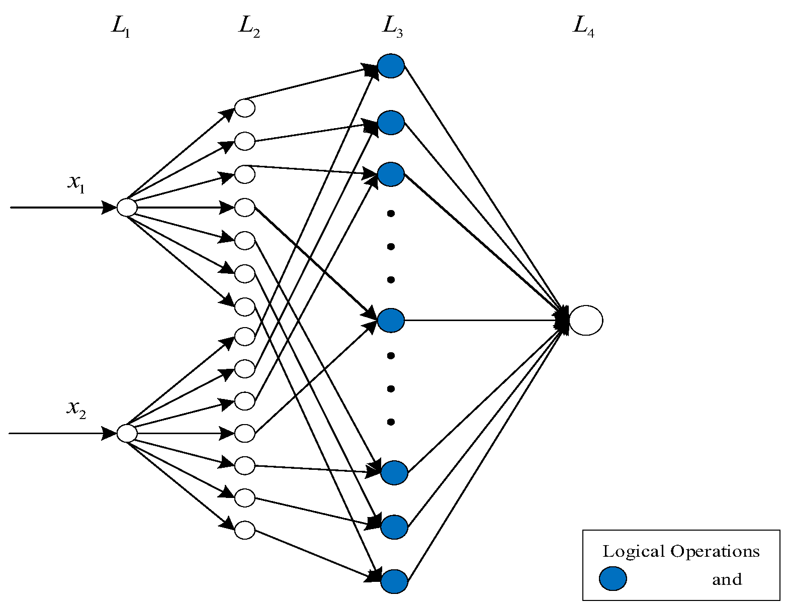
4.2.1. Controller Structure

Fuzzy RBF network has the advantages of radial basis neural network and fuzzy control, which improves the reasoning ability of the system [34]. Fuzzy neural network compensators are designed in three attitude channels, respectively, which is used to eliminate the dynamic inverse error caused by external interference of UAV. Based on the real-time output data of the flight control system, the compensator uses the fuzzy rules automatically generated by the neural network to approximate the controlled parameters online [35]. In this paper, the improved fuzzy neural network designed has four layers, including input layer $L_1$, fuzzification layer $L_2$, fuzzy reasoning layer $L_3$ and output layer $L_4$. Figure 3 shows the organizational structure of the fuzzy neural network. The specific functions of each layer are:

• L₁: The fuzzy neural network structure has two inputs, which are the error $e$ of the state variable in the attitude system and the error rate of change $ec$. Therefore, the number of neurons in this layer is $L_1=2$. At the same time, the input volume is transferred to the next layer. The input and output of this layer can be expressed as

  $$L_1(i)=x_i,i=1,2.$$

  (25)
• L₂: Fuzzy the variables transmitted by the above formula. Give the same fuzzy subset $[\mathrm{NB},\mathrm{NM},\mathrm{NS},\mathrm{ZO},\mathrm{PS},\mathrm{PM},\mathrm{PB}]$ to the two outputs of the $L_1$ layer. The number of nodes in this layer is $L_2=14$, and the membership function is selected as Gaussian.

  $$L_2(i,j)=\exp (-\frac{{(L_1(i)-Q_{ij})}^2}{{(S_j)}^2}), S_j={\left[\begin{array}{ccc}{S}_1& \cdots & S_7\end{array}\right]}^T,Q_{ij}=\left[\begin{array}{ccc}{Q}_{11}& \dots & Q_{17}\\ Q_{21}& \dots & Q_{27}\end{array}\right]$$

  (26)

The $i$ and $j$ are the number of input variables and fuzzy sets, respectively. $Q_{ij}$ and $S_j$ are the center and width of the membership function.

• L₃: This layer is connected with the $L_2$ node to generate corresponding fuzzy rules, and the number of nodes is $L_3=49$. The output of the node is obtained by multiplying all the inputs of the node by fuzzy operation. The nodes of this layer are called rule nodes, and each node has its corresponding fuzzy rules. The output of this layer can be expressed as:

  $$L_3(j)={\displaystyle \prod _{j=1}^N{L}_2(i,j)}.$$

  (27)
• L₄: After the defuzzification is completed, each node variable of this layer is transformed into the network output. The obtained data are transmitted to the flight control system. In this fuzzy neural network structure, $L_4=1$

  $$L_4=W^T{L}_3,$$

  (28)

  where $W^T$ is the connection weight matrix between the layer and the upper node, and $W^T={\left[\begin{array}{cccc}{W}_1& W_2& \cdots & W_{49}\end{array}\right]}^T$.

4.2.2. Approximation Algorithm of Fuzzy RBF Network

$y_d\left(k\right)$ and $y\left(k\right)$ represent the expected output and the actual output, respectively. Next, the performance index function of the fuzzy RBF network is:

$$J(k)=\frac{1}{2}{[y_d(k)-y(k)]}^2,$$

(29)

The weight vector is adjusted by gradient descent method to eliminate the error $e\left(k\right)$ between $y_d\left(k\right)$ and $y\left(k\right)$. Taking the performance index function $J\left(k\right)$ as a reference, it propagates in the reverse direction of the weight connection. The weights approach the ideal value while reducing $e\left(k\right)$ to zero. Denote the learning rate as $\alpha$, and introduce a momentum factor $\beta$ to speed up the convergence. The learning algorithm for adjusting the weights of the output layer is:

$$\Delta \omega (k)=-\alpha \frac{\partial J(k)}{\partial \omega }=-\alpha \frac{\partial J(k)}{\partial e(k)}\frac{\partial e(k)}{\partial y_d}\frac{\partial y_d}{\partial \omega }=\alpha e(k)L_3,$$

(30)

The weight learning algorithm is:

$$\omega (k)=\omega (k-1)+\Delta \omega (k)+\beta [\omega (k-1)-\omega (k-2)].$$

(31)

In the hidden layer neurons of the fuzzy neural network, the learning algorithm for the membership function to adjust the central parameters is as follows:

$$\begin{array}{l}\Delta c_{ij}=-\alpha \frac{\partial J(k)}{\partial c_{ij}}=-\alpha \frac{\partial J(k)}{\partial n_j^2}\frac{\partial n_j^2}{\partial c_{ij}}\\ =\alpha e(k)\frac{\partial y_d}{\partial n_j^2}\frac{2(x_i-c_{ij})}{b_{ij}^2}=\alpha e(k)\frac{\partial y_d}{\partial L_3}\frac{\partial L_3}{\partial L_2}\frac{\partial L_2}{\partial n_j^2}\frac{2(x_i-c_{ij})}{b_{ij}^2}=\alpha e(k)\omega L_3\frac{2(x_i-c_{ij})}{b_{ij}^2}\end{array}$$

(32)

where $n_j^2=-\frac{{(L_1(i)-c_{ij})}^2}{{(b_j)}^2}$. The learning algorithm of the center parameter is:

$$c_{ij}(k)=c_{ij}(k-1)+\Delta c_{ij}(k)+\beta [c_{ij}(k-1)-c_{ij}(k-2)].$$

(33)

The learning algorithm of the membership function to adjust the base width parameter is:

$$\begin{array}{l}\Delta b_j=-\alpha \frac{\partial J(k)}{\partial b_j}=-\alpha \frac{\partial J(k)}{\partial n_j^2}\frac{\partial n_j^2}{\partial b_j}\\ =-\alpha e(k)\frac{\partial y_d}{\partial n_j^2}\frac{2(x_i-c_{ij})}{b_j^3}=-\alpha e(k)\frac{\partial y_d}{\partial L_3}\frac{\partial L_3}{\partial L_2}\frac{\partial L_2}{\partial n_j^2}\frac{2(x_i-c_{ij})}{b_j^3}=-\alpha e(k)\omega L_3\frac{2(x_i-c_{ij})}{b_j^3}\end{array}$$

(34)

The learning algorithm of the base width parameter is:

$$b_j(k)=b_j(k-1)+b_j(k)+\beta [b_j(k-1)-b_j(k-2)].$$

(35)

4.3. Controller Analysis

The above research contents give the structure and approximation algorithm of fuzzy neural network. In order to verify its control effect, this section analyzes the performance of the controller. Replace the dynamic inverse error $\Delta (x,\dot{x},u,\widehat{u})$ with $\chi$.

$$\widehat{\chi }={\widehat{W}}^T{L}_3,$$

(36)

where ${\widehat{W}}^T$ is the estimated value of $W^T$. (24) can be rewritten as:

$$\dot{e}=\Lambda e+B[\widehat{\chi }-\chi ].$$

(37)

Take the optimal weight matrix as:

$$W^{*}=\arg \underset{W\in \Omega }{\min }[\sup |\widehat{\chi }-\chi ],$$

(38)

where $\Omega$ is the set of $W$.

The minimum approximation error is defined as:

$$\epsilon =\widehat{\chi }(x|W^{*})-\chi ,$$

(39)

Rewrite (37) as:

$$\dot{e}=\Lambda e+B[\widehat{\chi }-\chi +\widehat{\chi }(x|W^{*})-\widehat{\chi }(x|W^{*})],$$

(40)

Substitute (36) and (39) into (40) to obtain:

$$\dot{e}=\Lambda e+B[{(\widehat{W}-W^{*})}^T{L}_3+\epsilon ].$$

(41)

Define the Lyapunov function as:

$$V=\frac{1}{2}{e}^{T}pe+\frac{1}{2\beta }{(\widehat{W}-W^{*})}^T(\widehat{W}-W^{*}),$$

(42)

where $\beta$ is a positive constant and $P$ is a positive definite matrix satisfying the Lyapunov equation:

$${\Lambda }^{T}P+P\Lambda +Q=0,$$

(43)

Derivation with respect to time gives:

$$\begin{array}{l}\dot{V}=\frac{1}{2}{\dot{e}}^{T}Pe+\frac{1}{2}{e}^{T}P\dot{e}+\frac{1}{\beta }{(\widehat{W}-W^{*})}^T\dot{\widehat{W}}\\ =\frac{1}{2}{e}^T{\Lambda }^{T}Pe+B^T{[{(\widehat{W}-W^{*})}^T{L}_3+\epsilon ]}^{T}Pe\\ +\frac{1}{2}{e}^{T}P\Lambda e+\frac{1}{2}{e}^{T}P{B}^T{[{(\widehat{W}-W^{*})}^T{L}_3+\epsilon ]}^T+\frac{1}{\beta }{(\widehat{W}-W^{*})}^T\dot{\widehat{W}}\\ =-\frac{1}{2}{e}^{T}Qe+e^{T}P{B}^T{[{(\widehat{W}-W^{*})}^T{L}_3+\epsilon ]}^T+\frac{1}{\beta }{(\widehat{W}-W^{*})}^T\dot{\widehat{W}}\\ =-\frac{1}{2}{e}^{T}Qe+e^{T}PB\epsilon +{(\widehat{W}-W^{*})}^T{e}^{T}PB{L}_3+\frac{1}{\beta }{(\widehat{W}-W^{*})}^T\dot{\widehat{W}}\\ =-\frac{1}{2}{e}^{T}Qe+e^{T}PB\epsilon +\frac{1}{\beta }{(\widehat{W}-W^{*})}^T[\dot{\widehat{W}}+\beta e^{T}PB{L}_3]\end{array}$$

(44)

Take the adaptive law as:

$$\dot{\widehat{W}}=-\beta e^{T}PB{L}_3,$$

(45)

Substitute the adaptive law into (44)

$$\dot{V}=-\frac{1}{2}{e}^{T}Qe+e^{T}PB\epsilon .$$

(46)

Since the minimum approximation error $\epsilon$ can be taken as a sufficiently small value, and $-\frac{1}{2}{e}^{T}Qe\le 0$, it is concluded that $\dot{V}\le 0$.

4.4. Nonlinear Dynamic Inverse Controller

The attitude control structure diagram of system is shown in Figure 4. The mathematical model of the attitude system of UAV is described as the following affine nonlinear form:

$$\{\begin{array}{l}\dot{x}=f(x)+g(x)u+d(t)\\ y=h(x)\end{array}$$

(47)

where the nonlinear coupling torque $f(x)$ and the manipulated matrix $g(x)$ can be expressed as:

$$f(x)=\left[\begin{array}{c}\frac{I_Y-I_Z}{I_X}\dot{\theta }\dot{\psi }-\frac{J_r{\Omega }_r}{I_X}\dot{\theta }-\frac{k_4\dot{\varphi }}{I_X}\\ \frac{I_Z-I_X}{I_Y}\dot{\varphi }\dot{\psi }-\frac{J_r{\Omega }_r}{I_X}\dot{\varphi }-\frac{k_5\dot{\theta }}{I_Y}\\ \frac{I_X-I_Y}{I_Z}\dot{\varphi }\dot{\theta }-\frac{k_6\dot{\psi }}{I_Z}\end{array}\right],g(x)\left[\begin{array}{ccc}l/I_X& 0& 0\\ 0& l/I_Y& 0\\ 0& 0& l/I_Z\end{array}\right]$$

(48)

The control input variable is $u={\left[\begin{array}{ccc}{u}_2& u_3& u_4\end{array}\right]}^T$. The total disturbance of the system is defined as the sum of the inaccurate part of the model and the external disturbance, $d(t)=\Delta f(x)+\Delta g(x)u+w(t)$. The pseudo control variable $\widehat{v}$ is introduced in the design of the inverse controller, and the structure of $\widehat{v}$ is given in Formula (20). According to the previous research content, the output parts of the command filter $v_d$, the linear controller $v_{pd}$ and the fuzzy neural network controller $v_{fnn}$ have been obtained. Substituting it into (17) gives $\widehat{v}={\ddot{x}}_c+k_p\dot{e}+k_d\ddot{e}-{\widehat{W}}^T{L}_3$, so the control law of the nonlinear dynamic inverse is

$$u=g_{}^{-1}(x)[{\ddot{x}}_c+k_p\dot{e}+k_d\ddot{e}-{\widehat{W}}^T{L}_3-f(x)-d(t)].$$

(49)

5. Simulation Results

In the above sections, the design of the control law of the attitude system of UAV is completed. Through the analysis and derivation of the inverse error compensation, the feasibility of the designed controller is demonstrated theoretically. In addition, this paper conducts experiments on the designed nonlinear dynamic inverse controller with fuzzy neural network compensation in the simulation environment. By observing the flight status of the aircraft in a calm environment and under different interf-erence conditions, the experimental results are evaluated to further verify the effectiveness of the controller. The relevant parameters of the aircraft used in this paper are given in

Table 2. Aircraft parameters.

Parameter	Unit	Value	Parameter	Unit	Value
$m$	$\mathrm{kg}$	$1.5$	$I_Y$	$\mathrm{kg}\cdot {\mathrm{m}}^2$	$2.372\times {10}^{-3}$
$l$	$\mathrm{m}$	$0.4$	$I_Z$	$\mathrm{kg}\cdot {\mathrm{m}}^2$	$6.316\times {10}^{-2}$
$g$	${\mathrm{m}/\mathrm{s}}^2$	$9.81$	$k_t$		$3.23\times {10}^{-5}$
$I_X$	$\mathrm{kg}\cdot {\mathrm{m}}^2$	$2.372\times {10}^{-3}$	$k_d$		$8.1\times {10}^{-7}$

.

The stability control of the attitude system is extremely critical to keep the UAV flying smoothly. The rotation of the attitude angle under the action of strong coupling will also cause the corresponding displacement of UAV. It is required that the aircraft can fly according to the desired trajectory during the execution of the mission, so the role of the controller prevents errors from being generated. In order to highlight the superiority of the control system designed in this paper, it is compared with the experimental results using only conventional proportional-differential control and fuzzy adaptive control.

When designing a proportional-differential dynamic inverse controller $\left(\mathrm{PD}\text{-}\mathrm{DIC}\right)$, first take approximate values of $P$ and $D$ according to relevant experience. Next, according to the principle of $P$ and $D$ tuning, the parameters are adjusted many times through experiments. Finally, combined with the simulation results, the parameters are adjusted by trial and error until the best. The roll channel adjustment parameters are $k_p=5$, $k_d=2$, pitch channel adjustment parameters are $k_p=25,k_d=12$, and yaw channel adjustment parameters are $k_p=20,k_d=6$.

The fuzzy adaptive dynamic inverse controller $\left(\mathrm{FA}\text{-}\mathrm{DIC}\right)$ takes the error $e$ between the actual value and the expected value of the current attitude angle and its rate of change $ec$ as the input, and the output are control parameters $k_1$ and $k_2$. The fuzzy subsets of these four parameters are all $[NB,NM,NS,ZO,PS,PM,PB]$, which are defined as “negative large, negative medium, negative small, zero, positive small, positive medium, positive large”. Suppose the input fuzzy universe is $X_i=[-r_i,r_i](i=e,ec)$ and the output fuzzy universe is $Y_z=[-c_z,c_z](z=k_1,k_2)$, where $r=3$, $c_{k_1}=0.3$, and $c_{k_2}=3$. Taking the pitch channel as an example, the three-dimensional curve diagram of the control parameters is shown in Figure 5.

5.1. Dynamic Response Characteristic Experiment

The performance of the three controllers is compared in a steady atmospheric environment. The altitude channel is independent. Refer to the attitude system and adopt the same control method for the altitude channel. Set the flying height of the quadrotor UAV at 20 m, and the flight time is 15 s. The simulation results are shown in Figure 6. The three attitude angles are turned to the desired angle value ${\left[{\begin{array}{ccc}{\varphi }_d& {\theta }_d& \psi \end{array}}_d\right]}^T={\left[\begin{array}{ccc}0.5& 0.5& 0.5\end{array}\right]}^T$, and they return to the initial state after being held in the air for 5 s. In the tenth second of the experiment, the step signal is added as a sudden disturbance, which makes the simulated flight environment of UAV more realistic. The aircraft keeps hovering in the air after being stabilized by the controller. The simulation results are shown in Figure 7.

Figure 6 shows the altitude channel flight test effect. The maximum overshoot, rise time, settling time and recovery time after being disturbed are used as the performance indicators to judge the control system. After measurement and simple calculation, the detailed values of these index parameters are shown in

Table 3. Performance metrics of controllers in the altitude channel.

Controller	Maximum Overshoot	Rise Time(s)	Settling Time(s)	Steady-State Error
$\mathrm{PD}\text{-}\mathrm{DIC}$	31.6%	0.231	2.577	5%
$\mathrm{FA}\text{-}\mathrm{DIC}$	0%	0.663	1.242	0%
$\mathrm{FNN}\text{-}\mathrm{DIC}$	0%	0.142	0.271	0%

. It is not difficult to see that there is no overshoot in $\mathrm{FA}\text{-}\mathrm{DIC}$ and $\mathrm{FNN}\text{-}\mathrm{DIC}$. However, under the premise of ensuring system stability, $\mathrm{FNN}\text{-}\mathrm{DIC}$ performs better, which is attributed to its shorter settling time and recovery time. Although the speed of the aircraft reaching the expected altitude in the $\mathrm{PD}\text{-}\mathrm{DIC}$ is faster than $\mathrm{FA}\text{-}\mathrm{DIC}$, there will be a slight error between the actual flying altitude and the expected altitude. In addition, the overshoot is large, resulting in its adjustment time is much higher than that of the other two control methods.

Similarly, in the control effects of the roll channel, pitch channel and yaw channel, only PD-DIC has an overshoot.

Table 4. Performance metrics of the three controllers of the attitude system.

Parameter Name	Channel	$\mathbf{P}\mathbf{D}\text{-}\mathbf{D}\mathbf{I}\mathbf{C}$	$FA\text{-}DIC$	$FNN\text{-}DIC$
Maximum Overshoot	Roll	5%	0%	0%
	Pitch	6.6%	0%	0%
	Yaw	9.34%	0%	0%
Settling Time(s)	Roll	2.377	0.694	0.399
	Pitch	2.738	0.558	0.252
	Yaw	1.515	0.518	0.133
Recovery Time(s)	Roll	2.269	0.507	0.271
	Pitch	2.410	0.505	0.219
	Yaw	1.324	0604	0.140

shows the comparison of performance indexes and parameters of the attitude system in three control modes. Generally speaking, the quadrotor under $\mathrm{FNN}\text{-}\mathrm{DIC}$ has obviously better flight performance.

5.2. Attitude Angle Tracking Experiment without Interference

In addition to hovering and take-off commands, quadrotor UAV needs to fly at a specified attitude angle when it performs its mission at high altitudes. To further compare the tracking performance of the three control methods for the attitude system, given the expected input value, the simulation experiment was carried out without external interference. The desired input for the roll angle is ${\varphi }_d=0.5\sin (0.8t)\cos (0.3t)$, the desired input for the pitch angle is ${\theta }_d=0.5\sin (0.8t)[1-\sin (0.7t)]$, and the desired input for the yaw angle is ${\psi }_d=0.5\sin (0.3t)\sin (0.8t)$. All the attitude angle channels adopt three control methods, and the tracking results are shown in Figure 8, Figure 9 and Figure 10.

It can be clearly seen that even in a stable and ideal environment, the $\mathrm{PD}\text{-}\mathrm{DIC}$ method cannot guarantee that UAV can accurately follow the desired trajectory. Tracking errors always exist in the roll, pitch and yaw channels. In contrast, $\mathrm{FA}\text{-}\mathrm{DIC}$ and $\mathrm{FNN}\text{-}\mathrm{DIC}$ can almost perfectly track the desired angle input value, and the control effect is ideal. The $\mathrm{FNN}\text{-}\mathrm{DIC}$ has a slight advantage in the control of roll and yaw angles.

5.3. Attitude Angle Experiment under Turbulent Disturbance

To fit the flight conditions in the actual environment, the atmospheric turbulence sequence established in the second section of this paper is used to simulate the interference suffered by UAV in the external flight, and then the experiment is carried out. Figure 11 shows the results of the influence of atmospheric turbulence on roll angle tracking. Figure 12 shows the results of the influence of atmospheric turbulence on pitch angle tracking. Figure 13 shows the results of the influence of atmospheric turbulence on yaw angle tracking. Obviously, the pitch angle is most affected by the atmospheric turbulence. PD-DIC seeks to make the controlled object be intensively adjusted in the shortest time, while there will be adjustment static error. It cannot perform adaptive control perfectly when there is external disturbance, and the anti-interference ability to the outside world is weak, so the tracking error always exists in the attitude channel. When encountering strong external interference, the control effect of $\mathrm{PD}\text{-}\mathrm{DIC}$ drops sharply because of the limitation of its own algorithm. Especially in the control of the pitch angle, it shows obvious tracking error and becomes difficult to keep stable. Compared with the almost ideal tracking effect in a calm atmosphere, Fuzzy-A also has a relatively obvious jitter phenomenon when dealing with the disturbance of quadrotor UAV by atmospheric turbulence. FNN introduces the learning ability of the neural network into the fuzzy system, and uses the distributed neural network to represent the fuzzy processing, fuzzy reasoning and fuzzy calculation of the fuzzy system. The experimental results show that FNN can still track the desired input value of the attitude angle in the case of strong external disturbance,

Table 5. Maximum tracking error of attitude angle under atmospheric turbulence.

Channel	$\mathbf{PD}\text{-}\mathbf{DIC}$	$FA\text{-}DIC$	$FNN\text{-}DIC$
$\mathrm{Roll} (°)$	0.098	0.013	0.006
$\mathrm{Pitch} (°)$	0.625	0.127	0.032
$\mathrm{Yaw} (°)$	0.047	0.011	0.003

.

6. Conclusions and Outlook

In this paper, the fuzzy neural network dynamic inverse controller is designed to solve the problems of poor attitude stability and difficult adjustment of the controller caused by the disturbance of atmospheric turbulence when quadrotor UAV performs tasks at sea level or complex terrain. Considering that atmospheric turbulence is a very complex physical phenomenon, the component model of atmospheric turbulence is firstly obtained based on the Dryden model. In the second chapter, the nonlinear dynamic model of UAV is established according to the Newton-Euler equation, and the atmospheric turbulence is added into the model as a disturbance. The third chapter adopts the method of dynamic inverse to cancel the nonlinear characteristics of the controlled object. The fuzzy neural network compensator is designed to eliminate the model inverse error caused by external disturbance. Finally, the designed controller is verified on the experimental platform, and in order to show its advantages, the $\mathrm{PD}\text{-}\mathrm{DIC}$ method and the FA-DIC method are added to compare the effects. The experimental results show that the dynamic response performance of the $\mathrm{FNN}\text{-}\mathrm{DIC}$ method and the stability in strong disturbance environment are better than the other two control methods.

In future work, the impact of low-altitude wind shear on further UAVs needs to be further considered. The nonlinear model of quadrotor UAV will be decoupled and analyzed by combining time scale separation and state feedback. According to the motion, the state variables of the system are divided into multiple loops, and then the control laws between the loops are independently designed. In addition, actual test flight experiments will be conducted in a real environment.

References

1. Tran, V.P.; Santoso, F.; Garrat, M.A.; Anavatti, S.G. Neural network-based self-learning of an adaptive strictly negative imaginary tracking controller for a quadrotor transporting a cable-suspended payload with minimum swing. IEEE Trans. Ind. Electron. 2021, 68, 10258–10268. [Google Scholar] [CrossRef]
2. Kim, S.; Kim, D.; Jeong, S.; Ham, J.W.; Lee, J.K.; Oh, K.Y. Fault diagnosis of power transmission lines using a uav-mounted smart inspection system. IEEE Access 2020, 8, 149999–150009. [Google Scholar] [CrossRef]
3. Zhang, H.T.; Hu, B.B.; Xu, Z.C.; Cai, Z.; Liu, B.; Wang, X.D.; Geng, T.; Zhong, S.; Zhao, J. Visual navigation and landing control of an unmanned aerial vehicle on a moving autonomous surface vehicle via adaptive learning. IEEE Trans. Neural Netw. Learn. Syst. 2021, 32, 5345–5355. [Google Scholar] [CrossRef] [PubMed]
4. He, H.X.; Duan, H.B. A multi-strategy pigeon-inspired optimization approach to active disturbance rejection control parameters tuning for vertical take-off and landing fixed-wing uav. Chin. J. Aeronaut. 2022, 35, 19–30. [Google Scholar] [CrossRef]
5. Wang, C.L.; Herbst, A.; Zeng, A.J.; Wongsuk, S.; Qiao, B.Y.; Qi, P.; Bonds, J.; Overbeck, V.; Yang, Y.; Gao, W.L.; et al. Assessment of spray deposition, drift and mass balance from unmanned aerial vehicle sprayer using an artificial vineyard. Sci. Total Environ. 2021, 777, 14. [Google Scholar] [CrossRef]
6. Nguyen, N.P.; Park, D.; Ngoc, D.N.; Xuan-Mung, N.; Huynh, T.T.; Nguyen, T.N.; Hong, S.K. Quadrotor formation control via terminal sliding mode approach: Theory and experiment results. Drones 2022, 6, 172. [Google Scholar] [CrossRef]
7. Liu, Q.; Chen, S.D.; Wang, G.B.; Lan, Y.B. Drift evaluation of a quadrotor unmanned aerial vehicle (uav) sprayer: Effect of liquid pressure and wind speed on drift potential based on wind tunnel test. Appl. Sci. 2021, 11, 7258. [Google Scholar] [CrossRef]
8. Najm, A.A.; Ibraheem, I.K. Altitude and attitude stabilization of uav quadrotor system using improved active disturbance rejection control. Arab. J. Sci. Eng. 2020, 45, 1985–1999. [Google Scholar] [CrossRef]
9. Ji, H.L.; Chen, R.L.; Li, P. Real-time simulation model for helicopter flight task analysis in turbulent atmospheric environment. Aerosp. Sci. Technol. 2019, 92, 289–299. [Google Scholar] [CrossRef]
10. Meenu, R.N.; Sunilkumar, K.; Singh, V.P.; Pandithurai, G.; Kalapureddy, M.C.R. Atmospheric turbulence characteristics in the troposphere and lower stratosphere of core monsoon zone. Atmos. Res. 2022, 279, 14. [Google Scholar] [CrossRef]
11. Andrade, F.A.A.; Guedes, I.P.; Carvalho, G.F.; Zachi, A.R.L.; Haddad, D.B.; Almeida, L.F.; de Melo, A.G.; Pinto, M.F. Unmanned aerial vehicles motion control with fuzzy tuning of cascaded-pid gains. Machines 2022, 10, 12. [Google Scholar] [CrossRef]
12. El Gmili, N.; Mjahed, M.; El Kari, A.; Ayad, H. Particle swarm optimization based proportional-derivative parameters for unmanned tilt-rotor flight control and trajectory tracking. Automatika 2020, 61, 189–206. [Google Scholar] [CrossRef]
13. Song, J.; Hu, Y.; Su, J.; Zhao, M.; Ai, S. Fractional-order linear active disturbance rejection control design and optimization based improved sparrow search algorithm for quadrotor uav with system uncertainties and external disturbance. Drones 2022, 6, 229. [Google Scholar] [CrossRef]
14. Kaba, A. Improved pid rate control of a quadrotor with a convexity-based surrogated model. Aircr. Eng. Aerosp. Technol. 2021, 93, 1287–1301. [Google Scholar] [CrossRef]
15. Elkhatem, A.S.; Engin, S.N. Robust lqr and lqr-pi control strategies based on adaptive weighting matrix selection for a uav position and attitude tracking control. Alex. Eng. J. 2022, 61, 6275–6292. [Google Scholar] [CrossRef]
16. Smeur, E.J.J.; de Croon, G.; Chu, Q. Cascaded incremental nonlinear dynamic inversion for mav disturbance rejection. Control Eng. Pract. 2018, 73, 79–90. [Google Scholar] [CrossRef] [Green Version]
17. Zheng, B.C.; Wu, Y.W.; Li, H.; Chen, Z.P. Adaptive sliding mode attitude control of quadrotor uavs based on the delta operator framework. Symmetry 2022, 14, 498. [Google Scholar] [CrossRef]
18. Ahmed, N.; Shah, S.A.A. Adaptive output-feedback robust active disturbance rejection control for uncertain quadrotor with unknown disturbances. Eng. Comput. 2022, 39, 1473–1491. [Google Scholar] [CrossRef]
19. Yang, W.; Cui, G.Z.; Li, Z.; Tao, C.B. Fuzzy approximation-based adaptive finite-time tracking control for a quadrotor uav with actuator faults. Int. J. Fuzzy Syst. 2022, 24, 3756–3769. [Google Scholar] [CrossRef]
20. Zhang, Y.; Chen, Z.Q.; Sun, M.W. Trajectory tracking control for a quadrotor unmanned aerial vehicle based on dynamic surface active disturbance rejection control. Trans. Inst. Meas. Control 2020, 42, 2198–2205. [Google Scholar] [CrossRef]
21. Noordin, A.; Mohd Basri, M.A.; Mohamed, Z.; Mat Lazim, I. Adaptive pid controller using sliding mode control approaches for quadrotor uav attitude and position stabilization. Arab. J. Sci. Eng. 2020, 46, 963–981. [Google Scholar] [CrossRef]
22. Li, K.W.; Wei, Y.R.; Wang, C.; Deng, H.B. Longitudinal attitude control decoupling algorithm based on the fuzzy sliding mode of a coaxial-rotor uav. Electronics 2019, 8, 107. [Google Scholar] [CrossRef] [Green Version]
23. Sun, C.; Liu, M.; Liu, C.a.; Feng, X.; Wu, H. An industrial quadrotor uav control method based on fuzzy adaptive linear active disturbance rejection control. Electronics 2021, 10, 376. [Google Scholar] [CrossRef]
24. Muthusamy, P.K.; Garratt, M.; Pota, H.; Muthusamy, R. Real-time adaptive intelligent control system for quadcopter unmanned aerial vehicles with payload uncertainties. IEEE Trans. Ind. Electron. 2022, 69, 1641–1653. [Google Scholar] [CrossRef]
25. Muliadi, J.; Kusumoputro, B. Neural network control system of uav altitude dynamics and its comparison with the pid control system. J. Adv. Transp. 2018, 2018, 3823201. [Google Scholar] [CrossRef]
26. Kayacan, E.; Khanesar, M.A.; Rubio-Hervas, J.; Reyhanoglu, M. Learning control of fixed-wing unmanned aerial vehicles using fuzzy neural networks. Int. J. Aerosp. Eng. 2017, 2017, 5402809. [Google Scholar] [CrossRef] [Green Version]
27. Wai, R.J.; Prasetia, A.S. Adaptive neural network control and optimal path planning of uav surveillance system with energy consumption prediction. IEEE Access 2019, 7, 126137–126153. [Google Scholar] [CrossRef]
28. Sarabakha, A.; Imanberdiyev, N.; Kayacan, E.; Khanesar, M.A.; Hagras, H. Novel levenberg-marquardt based learning algorithm for unmanned aerial vehicles. Inf. Sci. 2017, 417, 361–380. [Google Scholar] [CrossRef] [Green Version]
29. Tran, V.P.; Mabrok, M.A.; Garratt, M.A.; Petersen, I.R. Hybrid adaptive negative imaginary- neural-fuzzy control with model identification for a quadrotor. IFAC J. Syst. Control 2021, 16, 100156. [Google Scholar] [CrossRef]
30. Rai, S.N.; Jawahar, C.V. Removing atmospheric turbulence via deep adversarial learning. IEEE Trans. Image Process. 2022, 31, 2633–2646. [Google Scholar] [CrossRef] [PubMed]
31. Jiang, Z.X.; Yang, L.B.; Wang, D.; Tang, Y.M. Modeling and controller design of tilt-rotor uav under wind disturbance. Flight Dyn. 2021, 39, 38–44. [Google Scholar] [CrossRef]
32. Wang, B.; Shen, Y.; Zhang, Y. Active fault-tolerant control for a quadrotor helicopter against actuator faults and model uncertainties. Aerosp. Sci. Technol. 2020, 99, 105745. [Google Scholar] [CrossRef]
33. Liu, X.Y.; Wang, W.T.; Wang, Y.D.; Shao, C.; Cong, Q.M. Coordinated optimization control of shield machine based on dynamic fuzzy neural network direct inverse control. Trans. Inst. Meas. Control 2021, 43, 1445–1451. [Google Scholar] [CrossRef]
34. Rao, J.; Li, B.; Zhang, Z.; Chen, D.; Giernacki, W. Position control of quadrotor uav based on cascade fuzzy neural network. Energies 2022, 15, 1763. [Google Scholar] [CrossRef]
35. Yu, H.; Lu, J.; Zhang, G.Q. Topology learning-based fuzzy random neural networks for streaming data regression. IEEE Trans. Fuzzy Syst. 2022, 30, 412–425. [Google Scholar] [CrossRef]
Figure 1. Free atmospheric turbulence components. (a) U-direction, (b) V-direction, and (c) W-direction.
Applsci 12 12232 g001
Figure 2. Structure and coordinate transformation of quadrotor UAV.
Applsci 12 12232 g002
Figure 3. Fuzzy Neural Network Structure.
Applsci 12 12232 g003
Figure 4. Attitude control structure diagram of system.
Applsci 12 12232 g004
Figure 5. Three-dimensional curve diagram of the control parameters: (a) k 1 , (b) k 2 .
Applsci 12 12232 g005
Figure 6. Experimental results of three controllers on altitude channel.
Applsci 12 12232 g006
Figure 7. The control effect of the three kinds of controllers in a stable atmosphere: (a) roll channel, (b) pitch channel, and (c) yaw channel.
Applsci 12 12232 g007
Figure 8. The results of the roll angle trajectory tracking. (a) Roll angle tracking track, and (b) roll angle tracking error.
Applsci 12 12232 g008
Figure 9. The results of the pitch angle trajectory tracking. (a) Pitch angle tracking track, and (b) pitch angle tracking error.
Applsci 12 12232 g009
Figure 10. The results of the yaw angle trajectory tracking. (a) Yaw angle tracking track, and (b) yaw angle tracking error.
Applsci 12 12232 g010
Figure 11. Roll angle tracking results under atmospheric disturbance: (a) Roll angle tracking curve, and (b) tracking error curve.
Applsci 12 12232 g011
Figure 12. Pitch angle tracking results under atmospheric disturbance: (a) Pitch angle tracking curve, and (b) tracking error curve.
Applsci 12 12232 g012
Figure 13. Yaw angle tracking results under atmospheric disturbance: (a) Yaw angle tracking curve, and (b) tracking error curve.
Applsci 12 12232 g013