Abstract
In this work, we introduce a new workflow to solve portfolio optimization problems on annealing platforms. We combine a classical preprocessing step with a modified unconstrained binary optimization (QUBO) model and evaluate it using simulated annealing (classical computer), digital annealing (Fujitsu’s Digital Annealing Unit), and quantum annealing (D-Wave Advantage). Starting from Markowitz’s theory on portfolio optimization, our classical preprocessing step finds the most promising assets within a set of possible assets to choose from. We then modify existing QUBO models for portfolio optimization, such that there are no limitations on the number of assets that can be invested in. Furthermore, our QUBO model enables an investor to also place an arbitrary amount of money into each asset. We apply this modified QUBO to the set of promising asset candidates we generated previously via classical preprocessing. A solution to our QUBO model contains information about what percentage of the whole available capital should be invested into which asset. For the evaluation, we have used publicly available real-world data sets of stocks of the New York Stock Exchange as well as common ETFs. Finally, we have compared the respective annealing results with randomly generated portfolios by using the return, variance, and diversification of the created portfolios as measures. The results show that our QUBO formulation is capable of creating well-diversified portfolios that respect certain criteria given by an investor, such as maximizing return, minimizing risk, or sticking to a certain budget.
1. Introduction
To this day, a multitude of highly relevant problems are thought to be intractable. This means that there are currently no known exact algorithms that can solve every instance of those problems in a worst-case polynomial time span. Due to the lack of exact algorithms, stochastic and heuristic algorithms inspired by nature, such as simulated annealing (SA), genetic algorithms (GA), swarm intelligence methods, and many more, have been developed. Those heuristic methods may not always find an optimal solution; however, in some cases they may yield a sufficiently good answer in a significantly shorter time span compared to known exact algorithms.
Based on several successful developments in the past decade, another tool to solve certain currently hard-to-solve problems has become available: quantum computing. Quantum computing itself, as a theoretical concept of performing calculations, has been known for decades. However, it was not clear whether quantum computers could eventually be built or not. Since the first machines potentially able to harness quantum phenomena to perform calculations became available in the last decade, intensive research efforts have been directed to understand these new computational possibilities. In theory, quantum computers promise to solve currently intractable problems, such as the factoring of numbers (see Shor’s algorithm [1]), in polynomial time. However, currently available quantum computers suffer from noise, missing error correction, low numbers of qubits, and more, and are thus far from reaching the theoretically possible speedups.
Current research efforts can be split into two main classes. The first class is concerned with the investigation of possible near-term advantages using currently available quantum and classical hardware. The second class is concerned with the creation of quantum algorithms that may exhibit speedups over current classically available algorithms, but require so-called fault-tolerant quantum hardware.
Commercially available quantum computers can also be split into two main classes: quantum annealers and quantum-gate computers. The former, manufactured for example by D-Wave Systems, are based upon the adiabatic theorem to perform calculations. Many of the (decision) problems currently thought to be intractable have an optimization version that can easily be mapped onto the native input format of quantum annealers, namely the Ising model (or the equivalent QUBO model). As of now, these models have become a quasi-standard for examining NP-complete and NP-hard problems in the realm of quantum computing. There is a plethora of known transformations for NP-complete/-hard problems to the QUBO model (see e.g., [2]), as well as guidelines on how to formulate QUBO models in general (see e.g., [3]). The performance of various QUBO formulations for certain problems has been subject to intensive investigations in the past couple of years (see e.g., [4,5,6,7,8,9,10,11]) and is still an ongoing effort.
In this paper, we focus on the applicability of annealing techniques to the NP-hard problem of portfolio optimization [5], a well-known topic for investment funds and individual investors.
The pioneering work by Harry Markowitz [12] in 1952 can be considered the foundation of portfolio optimization. The goal here is to distribute an investor’s capital on assets such that a given objective, such as maximizing the return or minimizing the risk, is optimized. Portfolio optimization is an actively researched question in scientific domains such as combinatorial optimization [13], operations research [14], data science [15], and the application of quantum computing [16]. Not only the academic community is focusing on this topic, but it is also a core business of banks and financial advisers and the combination of portfolio optimization with quantum techniques is addressed by numerous companies and consultants [17,18].
Current approaches of solving portfolio optimization with annealing techniques (see [5,11,19,20,21]) exhibit, amongst others, the following limitations:
- Limited amount of assets to choose from;
- Use of naive investment strategies for the calculation of future returns.
These approaches also try to solve portfolio optimization as a whole, which limits the possible problem sizes significantly, as current quantum hardware is not advanced enough yet to tackle bigger problems. Thus, we present a new workflow combining a classical preprocessing step with a modified QUBO model for portfolio optimization that is able to solve significantly larger optimization problems. In our modified QUBO model, we enable an investor to place an arbitrary amount of money into an arbitrary number of assets, which was not possible previously. The solutions to our QUBO model tell investors how to split their capital amongst available strategies in order to reach their goals (i.e., achieve a certain return and minimize risk). We evaluate our QUBO model via quantum annealing (QA), simulated annealing (SA), and digital annealing (DA).
This paper is organized as follows. First, we provide the reader with some preliminaries: in particular, we recall the foundations of portfolio optimization (Section 2), quantitative investing (Section 3), the QUBO model, and simulated and quantum annealing (Section 4). In Section 5 we give an overview of portfolio optimization in the field of quantum annealing. In Section 6 we present our approach to portfolio optimization followed by an evaluation in Section 7. The conclusion together with some discussion is given in Section 8.
2. Portfolio Optimization
Modern portfolio theory is about the optimal selection of assets for a given level of risk to achieve the maximal return [12]. This theory was first presented in 1952 by the pioneer in this field, Harry Markowitz [12]. His theory shows that investors should diversify their portfolios to achieve a maximum return under a given level of risk. The investors decide for themselves how to calculate the expected return and what return indicators are important. Suppose there are l assets. The expected return of a portfolio is given by
Variables with denote the portion of the asset i in the whole portfolio and is the expected return of asset i. Of course holds. The expected risk of a portfolio is given by
Here, denotes the covariance between assets i and j.
The investor has the possibility to select different combinations of . It is assumed that all combinations are distributed according to Figure 1. The x-axis represents the expected return (the more right the better) and the y-axis represents the expected risk (the lower the better):
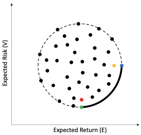
Figure 1.
Distribution of portfolios with E representing the expected return and V the expected risk. Figure inspired by [12].
The dashed/solid line in Figure 1 denotes the convex hull around a set of portfolios. That is, all envisioned portfolios lie inside that area. Every dot represents a single portfolio. The blue dot marks the portfolio where the expected return is the highest, while the portfolio marked with a green dot has got the lowest risk. As a trade-off for the lower risk, the portfolio represented by the green dot also yields lower expected returns than the portfolio represented by the blue dot. The solid part of the line in Figure 1 denotes the area where optimal portfolios may lie, which is also called the efficient frontier. Portfolios within the efficient frontier are considered optimal because they exhibit the best balance between maximizing the return E while also minimizing the risk V. The red dot, for example, is not optimal, because the green dot has a lower expected risk with the same expected return. Similarly, the yellow dot has a lower expected return compared to the green dot with the same expected risk.
To find the best investment portfolios, the problem needs to be formulated as an optimization problem:
This is the constrained quadratic form of the portfolio theory of Markowitz. Out of l assets, the ones with the lowest covariance and highest return shall be selected. The weighted percent values describe how the different assets build up the solution portfolio [5].
3. Quantitative Investment Strategies
Quantitative trading can be defined as the systematic implementation of trading strategies that humans create through rigorous research. In this context, systematic is defined as a disciplined, methodical, and automated approach [22] (p. 15).
The quantitative investment process starts by testing a possible strategy. Therefore, one has to start by gathering the necessary historical data, which might contain several flaws. For example, the data might be not adjusted to stock splits or dividends, there might be missing values, reported values might not be correct, and so on. If this is the case, one has to include a data cleaning step before one proceeds [22] (pp. 135–136). After establishing the data set for the potential strategy, the strategy is fitted to the historical data. There are additional pitfalls that need to be considered. For example, a historical database of stock prices might not include stocks that have “disappeared” due to bankruptcies, delistings, mergers, or acquisitions, and thus suffer from a so-called survivorship bias, because only “survivors” of those often unpleasant events remain in the database [23] (p. 33). Another example of a possible bias is the so-called data-snooping bias. This bias can be thought of as a kind of overfitting of the parameters to given historical data. It occurs when one tries to optimize the parameters of a strategy such that it performs exceptionally well on historical data. It is very likely that such an optimization can be performed [23] (p. 35). The look-ahead bias is about situations where information is used that was only available after the investment has been made. This information was not available when an asset was bought or sold [23] (p. 58). After the strategy shows acceptable performance on historical data, the strategy is tested on an out-of-sample data set, usually taken from the near past. Finally, the out-of-sample test (so-called backtest) is evaluated, and the strategy will either be used for investments or discarded [23] (p. 29).
In our work, the price series of assets are the foundation of a trend strategy and a mean reversion strategy. Trend strategies (also called momentum strategies) are based on the theory that sometimes markets move long enough in one direction such that the trend can be identified and exploited. Mean reversion strategies assume, however, that there exists a center of a price series (e.g., the mean of a price) and that the price including its fluctuation always returns to its center [22] (pp. 39–45). The price series must be stationary for a mean reversion strategy. Stationarity can mathematically be tested by the augmented Dickey–Fuller (ADF) test [24] (p. 49). Price changes in a price series are described as
The ADF test finds out if . If the hypothesis can be rejected, then the next price change depends on . Therefore, the series is not a random walk. The test statistics is the regression coefficient divided by the standard error of the regression . Since mean reversion is expected, must be negative and lower than the critical z- of the hypothesis. Variable k denotes price lags of the price series, is the constant drift of the price series, and is the auto-regressive parameter. Error term is independent and identically distributed with a mean of 0. Intuitively formulated, being a stationary price series means that the price moves away from its initial value slower than a geometric random walk. The speed of this moving can mathematically be calculated by the variance
in which z is the log price , an arbitrary point in time, and the average over all ts. For a geometric random walk the following is known:
Notation ∼ indicates that the relation for large becomes equality and for small the relation deviates from a constant line. If the price series is mean reverting or in a trend, then the formula is the following:
Here, H is the Hurst exponent with a value of for a geometric random walk, for a stationary price series, and for a trend. The trend or stationarity is stronger the larger the difference of H from [24] (p. 51).
Since price series are finite sets, the statistical significance of H must be determined. The hypothesis test for that is the variance ratio test [24] (p. 52), and it tests if
The null hypothesis is that the price series is a random walk. If the test equals 1, then a random walk can be rejected; if the test equals 0, then the series may be a random walk. The p-value of the test gives the probability that the null hypothesis can be accepted [24] (p. 52).
Variable in the ADF test formula (Equation (4)) is a measure for the time a price series needs to return to its center, also called half-life. For that, the price series must be transformed into its differential form. For this, the Ornstein–Uhlenbeck formula can be used:
where represents Gaussian noise. If is positive, then the price series is not stationary, while a close to 0 means that it will take a long time until the series returns to its center. Additionally, the measure of half-life provides a guideline for how the period of the moving average and the moving standard deviation for strategies shall be selected. The period is optimal if it is a small portion of [24] (p. 53).
Most price series are not stationary, however, stationary portfolios can be created out of several distinct price series. This works via the cointegration of price series. Cointegration means that if a linear combination of non-stationary price series can be found, then they are cointegrated with each other. A common combination consists of two price series. Here, one price series is invested in long (an investor bought and owns the asset) and the other is invested with a factor (hedge ratio) in short (an investor lent and sold an asset and returns it later). That is called the pairs-trading strategy. To test the stationarity of the cointegration, the augmented Dickey–Fuller (ADF) test can be used. First, the optimal hedge ratio is calculated by linear regression
where S is the alleged stationary price series, h the hedge ratio, and are the two distinct series. Using S, a portfolio will be created. On top of the price series of the portfolio, the ADF test is executed to show stationarity. Not all pairs of series are suitable for a pairs-trading strategy. The mathematical techniques presented in this section are crucial for the preprocessing step in our portfolio optimization step. By the use of backtesting strategies on different assets and discarding strategies on assets where the backtest results are unsatisfactory, the search set for the portfolio optimization can be reduced. However, the complexity of the optimization problem still remains.
4. Annealing Methods and the QUBO Model
As we use different types of annealing methods for our evaluation, namely simulated annealing, quantum annealing, and digital annealing, we recall the necessary fundamentals in this section. All types of annealing methods are meta-heuristics designed to find the global optimum of a given optimization problem.
4.1. Simulated Annealing
Simulated annealing (SA) is named after its analogy to the process of physical annealing with solids, in which a crystalline solid is heated and then allowed to slowly cool down until it achieves its most regular crystal lattice configuration (i.e., its minimum lattice energy state), and thus is free of crystal defects. If the cooling schedule is sufficiently slow, the final configuration results in a solid with such a superior structural integrity [25]. Simulated annealing establishes the connection between this type of thermodynamic behavior and the search for a global optimum for a discrete optimization problem. Furthermore, it provides an algorithmic means for exploiting such a connection [25]. At each iteration of a simulated annealing algorithm applied to a discrete optimization problem, the values for two solutions (the current solution and a newly selected solution) are compared. Improving solutions are always accepted, while a fraction of non-improving (inferior) solutions are accepted in the hope of escaping local optima while continuing to search for a global optimum. The probability of accepting non-improving solutions depends on a temperature parameter, which is typically non-increasing with each iteration of the algorithm [25]. For an in-depth mathematical description of the simulated annealing idea, see [25,26].
4.2. Quantum Annealing
Quantum annealing (QA) is a heuristic method for solving combinatorial optimization problems, similar to simulated annealing [27]. Quantum annealing is a derivative of adiabatic quantum optimization [4], which is based on the time-dependent Schrödinger equation
where denotes the quantum mechanical wave function of an underlying physical system and is the time-dependent Hamiltonian that drives the dynamics [4]. A generic form of this Hamiltonian is
with and T being the final evolution time. The schedules are monotonic and satisfy and . Therefore, the quantum state evolves under an interpolation from to in order to prepare the final state . Assuming the initial state is an eigenstate of , then the adiabatic theorem promises that the quantum state will remain an instantaneous eigenstate of provided the dynamics evolve sufficiently slow. The latter condition may be enforced by choice of the annealing time T or the schedules. Consequently, we may select the final Hamiltonian to represent a computational problem in which the eigenstates encode a well-defined solution [4].
4.3. Digital Annealing
Digital annealing and the corresponding hardware the Fujitsu Digital Annealing Unit (DAU) are designed to solve fully connected quadratic unconstrained binary optimization (QUBO) problems. It is implemented on application-specific CMOS hardware and currently solves problems of up to 8192 variables [28]. The DAU’s algorithm is based on SA, but differs from it in two main ways: first, it uses a parallel-trial scheme in which each Monte Carlo step considers a flip of all variables (separately), in parallel. If at least one flip is accepted, one of the accepted flips is chosen uniformly at random and it is applied. The advantage of the parallel-trial scheme is that it can boost the acceptance probability, because the likelihood of accepting a flip out of N flips is typically much larger than the likelihood of flipping a particular variable. Parallel rejection algorithms on GPU (see [29,30]) are examples of similar efforts in the literature to address the low acceptance probability problem in Monte Carlo methods [28]. Finally, digital annealing employs an escape mechanism called dynamic offset, such that if no flip was accepted, the subsequent acceptance probabilities are artificially increased by subtracting a positive value from the difference in energy associated with a proposed move. This can help the algorithm to surmount short, narrow barriers [28]. For more details on digital annealing, see [28,31].
4.4. Quadratic Unconstrained Binary Optimization (QUBO)
The quadratic unconstrained binary optimization problem (QUBO) model has emerged as an underpinning of the quantum computing area known as quantum annealing (as well as digital annealing), and has also become a subject of study in neuromorphic computing [3]. Through these connections, QUBO models lie at the heart of experimentation carried out with quantum computers developed by D-Wave Systems and neuromorphic computers developed by IBM [3]. Furthermore, QUBO models can also be used as an input for algorithms such as QAOA [32], which can be executed on quantum-gate computers.
There are many well-known reductions of NP-hard and NP-complete problems to QUBO (see [2]), which itself is an NP-hard optimization problem [3]. We proceed to define QUBO as presented in [33]:
Given a graph with node set and edge set . Denoting the weight of edge by , we define QUBO as
with . An equivalent compact definition, where the coefficients of Equation (13) are represented as a matrix Q is
with and Q being an matrix of coefficients [33].
5. Related Work
There are several methods for portfolio optimization. The largest influence comes from Markowitz’s work [12] for portfolio selection. Probability and optimization theory is combined to find a portfolio with minimized risk and maximized return [34]. In the following paragraphs, existing portfolio optimization approaches using quantum methods are presented.
The portfolio optimization problem has been solved using two different quantum computing methods. The first method is the quantum linear systems algorithm. The algorithm creates a risk-return curve in which the portfolio with the lowest risk for a given return can be found [35]. The second method is quantum annealing. In the following, we will present existing quantum annealing approaches.
Elsokkary et al. [11] selected the expected price value of a stock as the return. For the risk measure, the variance of the stock price was used. Additionally, a budget for the portfolio can be chosen. The corresponding QUBO model consists of three parts.
The first part is for the expected return with depending if a stock i is selected for the portfolio or not. The second part represents the risk with , and if then it is the variance of the stock price. The third part constrains the model to a given budget B. is the price of the stock i. The positive weights describe how important each term in the model is. In the application of that approach, data from the Abu Dhabi securities exchange has been used, and the algorithm was executed on the D-Wave Quantum Annealer. The thetas were all set to 13 to have equal importance for the three terms. Given a budget of USD 100, their algorithm constructed a portfolio worth USD . Therefore, the thetas were adjusted to , , , and the constructed portfolio was worth USD , where no optimization for risk was made [11]. Their approach lacks the ability to have more than one stock for each security in the portfolio. Additionally, the authors did not mention how the expected return was calculated. Venturelli et al. [5] used a similar approach for portfolio optimization via quantum annealing. The authors used investment funds instead of stocks as assets, the annual return of each fund as the expected return, and the annual standard deviation of the logarithmic return as the risk. Using the two factors of return and risk, the Sharpe ratio was calculated for each fund in order to put each fund into one of the 12 classes for the “attractiveness” of the asset. The QUBO model has been defined as follows:
The attractiveness class of each fund is represented by , while indicates whether fund i is in the portfolio or not. is the covariance of the corresponding returns as a measure to construct a diversified portfolio:
Additionally, the approach has an extension to choose the amount of funds in the portfolio out of N funds. The amount of funds that shall be in the portfolio can be selected using M. P is a penalty that sets the global minimum of the function to the wanted amount such that . The approach was executed via quantum annealing and reverse quantum annealing. The results show that reverse annealing is 100 times faster than quantum annealing [5]. Their approach lacks the ability to tell the theoretical investor how much of the capital shall be invested into which fund. Their work did not show any portfolios constructed by the quantum annealer, instead, they just showed if the problem has been solved and in what time. Additionally, the expected return of each fund was computed naively by means of historical returns.
The approach by Phillipson and Bhatia [19] is similar to Venturelli et al. [5] and Elsokkary et al. [11]. N assets to invest in are available out of the Nikkei225 and S&P500. The expected return of asset i is calculated over a quarterly 5-year data period. The risk is modeled by a risk matrix , where the diagonal is the variance of each assets and the other cells represent the covariance of the assets. n determines how many assets shall be contained in the resulting portfolio. The return of the result portfolio shall be higher than and the approach searches for the portfolio out of n assets that achieves the target return with minimal risk. The corresponding QUBO formulation is as follows:
The lambdas weigh each term for its importance. The results in that approach only show how fast quantum annealing is compared to other optimization algorithms such as simulated annealing [19].
To conclude, existing approaches lack the ability to tell a theoretical investor how much of the capital needs to be allocated to which asset to have the optimal portfolio. Additionally, taking the mean of historical returns is a naive estimate of asset returns.
6. Portfolio Optimization Implementation
In this section, we will present our implementation of the portfolio optimization problem. First, the implementations of the pairs-trading strategy (Section 6.1) and trend-following strategy (Section 6.2) are presented. The strategies are backtested in a preprocessing step such that only certain strategies on specific stocks and ETFs are included in the possible solution set of the portfolio optimization. The preprocessing starts with the backtesting of both strategies. First, both strategies are applied to the historical price data from 2015 to 2019 of the stocks and ETFs. Then the returns of the strategies with their corresponding assets are saved for that timeframe. Next, the Sharpe ratio and variance based on these returns for all strategy/asset combinations are computed. The 18 strategy/asset combinations with the highest Sharpe ratios are saved and later used for portfolio optimization. Finally, our QUBO model is presented (Section 6.3) which is the central part for the different annealing heuristics.
6.1. Pairs-Trading Strategy
The pairs-trading strategy was implemented similarly to Chan et al. [24] (p. 56) to show how an investment strategy can be used in combination with annealing algorithms. Because most of the price series of assets are not stationary, cointegrated pairs of price series were used. If a linear combination of non-stationary price series can be found, then they are cointegrated. To find the stationary combinations, the ADF test was used. First, for every possible combination of distinct price series a linear regression was created. The regression coefficient tells how the pairs are combined. The idea is that if for example, one asset is 25% long, then the other one is 75% short. The regressions coefficient is the so-called hedge ratio. Next, the ADF test was executed on the combined price series to test whether the combined series is stationary. If that was the case, then the Hurst exponent was calculated to determine how strong the series’ stationarity is. Only strongly stationary series were used for further executions of the pairs trading strategy. Afterward, the remaining price series were tested in an out-of-sample data set. As parameters for the strategy the rolling mean and the rolling standard deviation of the series are needed. To calculate the rolling mean and rolling standard deviation, of the half-life was used for the rolling window size. For each data point of the price series, the Z-score in its distribution of returns was calculated. For simplification, we assumed that the returns follow a Gaussian distribution. The formula for calculating the z-score is:
If the z-score is in one of the two 25% confidence intervals, then a trade will be executed. The first price series of the pair will be invested long and the second short. The hedge ratio tells how much the second will be invested in short per unit of the first asset. At that moment the return of the cointegrated price series is on the edge of its return distribution. Because of the stationarity, the return will revert to its mean. As soon as the return comes back close to its mean, the trade will be finalized and both positions will be closed. For every transaction, transaction costs of 1% have been assumed. This includes commissions and fees for the US-American market of a broker (interactive brokers commissions, https://www.interactivebrokers.com/en/index.php?f=1590&p=stocks1, 29 August 2021). Slippage and market impact are not included because we only used percentages of the overall capital for the calculation of the positions. To model slippage and market impact, exact transaction amounts must be known. Out of the result of the backtest, the Sharpe ratio for every pair was calculated and it is used later on for the annealing. For the Sharpe ratio, a risk-free rate of % was used (YCharts, US 1 Year Treasury Rate, https://www.ycharts.com/indicators/1_year_treasury_rate, 29 August 2021). The risk-free rate is the return of the 1-year treasury bill of the US.
6.2. Trend-Following Strategy
The trend-following strategy was implemented again similarly to Chan et al. [24] (p. 138) to show how multiple investment strategies can be used with annealing algorithms. First, for every asset, the Hurste exponent was calculated to find price series that are in a trend. Afterward, the statistical significance of the price series was calculated because they are finite. If the Hurst exponent indicates a strong trend in one direction and the statistical significance was large enough, then the assets are used for further executions. Second, the parameters of this strategy were calculated. Those are the lookback and the holding period. The idea is that a price series is observed for the amount of time of the lookback period. Because the series is in a trend, an investment can be made for the amount of time of the holding period. To calculate both periods, the correlation coefficient for different pairs of periods was used. Additionally, the statistical significance of the correlation coefficient was calculated. The largest or smallest coefficient was used to determine the pair of periods. It is possible that after an increase or decrease of the lookback period of the asset price, the exact opposite happens for the holding period. Next, an out-of-sample backtest was executed as well. Every remaining asset with momentum was observed for the duration of the lookback period. Using the value of the return and the correlation coefficient, an investment was made long or short. For example, if a price series has a negative return during the lookback period and a negative correlation coefficient, the investment made was long. After the duration of the holding period, the position is sold. At this point in time the lookback period will be observed again, until the start of a new holding period is found. Transaction costs are the same as for the pairs-trading strategy. Out of the returns, the Sharpe ratio was calculated for the annealing.
6.3. QUBO Model
As a foundation for our QUBO model, the approaches of Venturelli et al. [5], Elsokkary et al. [11], and Palmer et al. [36] were used. In the approach of Venturelli et al., only a specific number of stocks can be selected. In our model, we lift this restriction and thus enable the investor to select an arbitrary amount of assets to invest in. With the approach of Elsokkary et al., only a single predefined amount of capital can be invested into an asset, or no money at all will be spent on this asset. In our model, we do not limit the investor to certain predefined amounts of money that can be invested into each asset, but enable the investor to spend an arbitrary amount of money on each asset. Palmer et al. incorporate logarithmic returns as well as a limitation of the amount of money that can be invested into a single asset in their QUBO model. The amount of money that can be invested into a single asset n in the approach of Palmer et al. is limited to the interval [, ]. The values and denote the percentage values with respect to the whole available budget, i.e., and are in the range [0, 1]. Palmer et al. introduce this limitation in order to foster the creation of diverse portfolios. In our approach, we do not incorporate logarithmic returns, but rather use the Sharpe ratio of the assets that we gained via our preprocessing step. We also do not limit an investor to certain ranges of amounts that the investor can spend on individual assets. In our evaluation (see Section 7), we will empirically show that lifting this restriction in our approach will still lead to the creation of a diverse portfolio. Thus, this restriction is not necessary for our QUBO model.
We now present our modifications to the approaches mentioned above. In our approach, we do not limit the number of stocks that can be invested in and we also enable investors to spend potentially arbitrary fractions of their capital on each strategy. A solution to our approach indicates which fraction of the whole capital should be spent on which strategy.
In our approach, we use 7 bits to express the available capital, similar to Ottaviani et al. [37]. Thus, a total fraction of of the whole capital can be spent on strategies of a portfolio. For each available strategy we introduce a 7-bit binary variable as
Binary variable is the least significant bit and binary variable is the most significant bit. Variable will denote which fraction of the whole capital should be spent on a certain strategy. The 7 bits, capable of representing different values from 0 to 127, is an arbitrary number that was chosen because it is the closest binary representation to the decimal number 100. For example, represents , meaning that no capital is invested in the corresponding strategy. The other extreme, namely , represents , meaning that the entire capital is invested in the corresponding strategy. If for example , then the fraction of the whole capital is spent on strategy . The goal of the portfolio optimization here is to allocate and distribute 100% () of the capital efficiently over different strategies to ensure diversification and lower risk. If an investor needs a more fine-grained breakdown of the capital, more than 7 bits can be used, resulting in a higher number than 127 and lower possible fractions than .
Similarly to Venturelli et al. [5], the attractiveness of an asset in our approach is measured by using the Sharpe ratio. However, in our approach, we do not cluster the Sharpe ratios into different classes with different weights, but use the nominal value of the Sharpe ratio. To calculate the Sharpe ratio of a strategy, we test the strategy on different assets and calculate the Sharpe ratio in accordance with the results of the backtest. We can now formulate the first part of our QUBO formulation. Suppose there are l strategies available. The following equation determines which fraction of the budget should be spent on which strategy, based on the Sharpe ratio of the respective strategy:
As explained, we dedicate 7 bits to each strategy in order to enable the approach to dedicate only a certain fraction of the whole capital to a strategy within a portfolio. Notice that the bits for constitute for one of the as introduced in Equation (20). Thus, in the above equation the Sharpe ratio of a single strategy is used 7 times. Hence, with , . The Sharpe ratio here is the value calculated by the backtesting of the preprocessing. As diversification is an important measure to reduce risks involved in investing, we add a second term that uses the covariance between different strategies, analogously to Venturelli et al. [5], which fosters the creation of well diversified portfolios.
To complete our approach, we add a final term, which penalizes both overspending and underspending of the available budget:
As this was the last step of our approach, the final QUBO formulation of our approach is given as
Remember, l denotes the number of available strategies, while parameters are weights to give more importance to different parts of the QUBO model. For example, to emphasize minimizing the risk, should be increased. As mentioned earlier, if the investor needs a finer breakdown of the capital, all 7s in Equation (24) needs to be replaced by the number of bits the investor needs. Additionally, in Equation (24), the value 127 needs to be replaced by the maximum number representable by the chosen number of bits.
6.4. Theoretical Remarks
In this subsection we provide a theoretical analysis of the preprocessing steps as well as the QUBO model regarding scalability and complexity. First, we describe our preprocessing of the pairs trading strategy, which is the process of finding all stationary asset pairs of all available assets, see the pseudocode in Algorithm 1.
| Algorithm 1 Pairs trading: find stationary pairs |
|
The procedure shown in Algorithm 1 has a time complexity of since we need to iterate over each asset and then through each other asset. Next for preprocessing, we need to execute a backtest to see how well a pairs trading strategy performs on all stationary pairs. Therefore, the actual strategy illustrated in Algorithm 2 is executed on the same timeframe as the assets used for Algorithm 1. The time complexity for that procedure is since we only have to iterate over each timestep of the backtest period. Therefore, the overall time complexity of the pairs trading preprocessing is
| Algorithm 2 Pairs trading strategy |
|
The trend-following strategy is executed on the same assets as the pairs trading strategy. The preprocessing procedure for the trend following strategy is described in Algorithm 3. It consists of two parts, first, for each asset we calculate the best lookback and holding period as well as their correlation coefficient as described in Section 6.2. Second, we execute the actual strategy based on the parameters found. The time complexity for that process is since we only have to iterate over each asset once.
| Algorithm 3 Trend following: preprocessing |
|
Now we will give some theoretical remarks to our QUBO formulation, see Equation (24). The procedures will fill the matrix entirely because the covariance between each asset is needed. Depending on the number of bits, as described in Equation (20), each asset occupies a number of variables equal to the number of bits. Therefore, the two dimensions of the QUBO matrix have a complexity of , where s is the number of strategies and b is the number of bits. It is not possible to make the resulting dense matrix more sparse, as it would contradict the goal of risk minimization in the original portfolio optimization problem. In order to minimize risk in a portfolio, the covariance between assets must be as close as possible to 0. That means that all assets in a portfolio are diverse and mitigate risk. Therefore, even if the QUBO matrix contains many 0s, they can not be eliminated because they are highly wanted. This fact makes portfolio optimization a computationally heavy problem and it shows the importance of new technologies such as quantum annealing or digital annealing.
7. Evaluation
We evaluate our new QUBO formulation for portfolio optimization by assuming a hypothetical investor who splits their money according to the suggestion of the QUBO optimization process and observing the development of their portfolio. We show that it is possible to add additional risk minimization, if needed, by adjusting the parameters of our model. The same is true for the maximization of the expected return.
7.1. Dataset
Our data set consists of stocks of the New York Stock Exchange (NYSE) as well as common exchange-traded funds (ETFs). The data set contains the daily adjusted closing prices of those stocks and respective ETFs over a period of 5 years, starting on 31 December 2014 and ending on 31 December 2019. The daily adjusted closing prices of each stock and respective ETF over the 5-year period form a price series. Since the data were not complete (e.g., daily closing prices were missing for several days for certain stocks or ETFs), we decided to only keep price series that contain more than 900 daily prices. All the data were acquired via Yahoo Finance.
7.2. Evaluation Framework
The experiments are carried out on D-Wave System’s Quantum Annealer (Advantage System 4.1), on Fujitsu’s Digital Annealing Unit (DAU Version 2), and on a classical computer using simulated annealing. We use default parameters for all algorithms on their respective hardware systems. We use UQO [38] as a platform to handle the execution of our experiments. Since D-Wave’s Advantage System 4.1 only provides about 5000 qubits, arranged in the Pegasus graph, we were only able to use 18 strategies. We chose 8 pairs-trading strategies on ETF pairs and 10 trend-following strategies on different NYSE stocks as our 18 strategies. Each of the 18 strategies were selected by the best Sharpe ratio of the backtest results. To compare the annealing results to a random process, we created randomized portfolios, each of them consisting of an arbitrary amount of strategies that were assigned an arbitrary fraction of the capital.
7.3. Diversification Measure
In the following figures to be seen, the coloring indicates the diversification of the portfolios. We used the following equation to determine the diversification of a portfolio:
In this equation, P denotes a portfolio, the price series of the portfolio are denoted by , , , and are the fractions of the capital that were invested into the strategies , in this specific portfolio P. In the denominator of the first part of the equation, we added the term to the entropy of the portfolio to prevent division by zero, as it might be possible that , which implies that all other weights must be zero, and thus the value of the denominator would be . Intuitively, the first part of the equation measures how similar the price series within the portfolio are, while the second part of the equation adds a reward for portfolios with a larger number of selected strategies. We normalize the result of the above diversification measure to the closed interval . The best value for diversification is 0, while and 1 denote the worst possible diversification. Here, 1 (dark-red coloring) means that all price series of the strategies in the portfolio behave exactly the same, while (dark-blue coloring) means that (groups of) time series behave exactly opposite, i.e., if the price of one series increases then the price of the other series decreases by the same amount. In our case, no portfolio received a normalized diversification result below 0, as none of the strategies within the created portfolios had negative correlation.
7.4. Results
We now present the results of our experiments. For all our experiments, we created 1000 random portfolios as well as samples for each of the annealing strategies simulated annealing, quantum annealing, and digital annealing. In our visualizations, we plot all the random portfolios, while for the portfolios generated with any of the annealing strategies we only plot the 10 best results. We start off by evaluating the created portfolios when using equal values for (weight for return) and (weight for risk).
Please note that in Figure 2 all portfolios generated by simulated annealing (marked as diamonds) and digital annealing (marked as stats) are almost stacked on top of each other, while portfolios generated by quantum annealing (crosses) reside in the same area as portfolios generated by simulated annealing and digital annealing, but exhibit an observable distribution. Nevertheless, the diversification, denoted by the coloring of the respective shapes, is roughly the same.
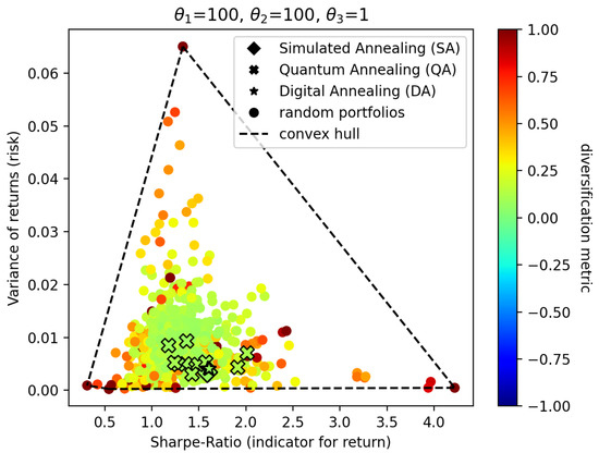
Figure 2.
Annealing results with equal weights for return and risk.
If we now increase to 400, which means we reward the creation of portfolios that yield higher returns, we obtain the results visualized in Figure 3. Note that there is nothing special about the value of 400, it is just an arbitrary value that emphasizes the creation of portfolios that yield higher returns.
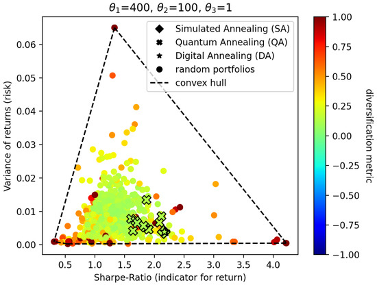
Figure 3.
Annealing results with increased weight on return.
The results show that, apart from a few outliers, the y-values of the annealing portfolios of Figure 2 and of Figure 3 are approximately equal. However, when comparing the results in Figure 2 to Figure 3, we can observe that the portfolios of the latter experiment possess a higher x-value. As the y-value indicates risk and the x-value indicates return, the conclusion is that while maintaining an equal amount of risk, the portfolios generated in Figure 3 yield a higher return.
In the next experiment, we increase to 1000 and decrease , which is the indicator for risk, to 1. This leads to portfolios that yield higher returns than previous experiments but also exhibit a lot more risk. The results of this experiment are visualized in Figure 4.
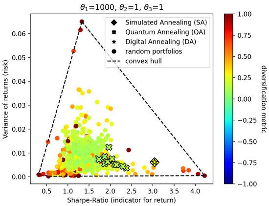
Figure 4.
Annealing results with increased weight on return and reduced weight on risk.
In this experiment, we observe that the resulting portfolios created by simulated annealing (diamonds) and digital annealing (stars) increase their Sharpe ratio as well as their risk significantly. One can also see that the color shifts from a greenish coloring in Figure 3 to a yellow color in Figure 4. These portfolios are less diversified than portfolios in the experiment of Figure 3. This is the intended effect of increasing the risk and the return. The portfolios generated by quantum annealing (crosses), however, only exhibit a slight trend towards increasing their Sharpe ratio. A significant change in risk can not be observed. One explanation for this might be that the decrease of from 100 to 1 is not significant enough for quantum annealing to mitigate influences such as noise or the additional scaling of parameters performed by the quantum annealer itself.
We now use the best portfolios generated by each of the annealing approaches in the previous experiment () to investigate the potential returns we would have received if we invested in these portfolios in the year 2020.
TPOR is the abbreviation of the ETF Direxion Daily Transportation Bull 3X Shares while DUSL is the abbreviation of the ETF Direxion Daily Industrials Bull 3X Shares. TPOR-DUSL in Figure 5 is a portfolio that only contains the pairs trading strategy with ETFs TPOR and DUSL. The pairs-trading strategy is long in the asset TPOR and short in the asset DUSL. Long in TPOR means that 75% of the investor’s capital is allocated to TPOR. Short in DUSL means that a number of stocks equal to 25% of the investor’s capital was borrowed from a bank, with the intention of selling it back to the bank at a later point in time. As can be seen in Figure 5, this portfolio lost approximately 60% of its value in 2020. The portfolios generated by the different annealing strategies have allocated between 23% to 25% of the investor’s total capital to TPOR-DUSL. Hence, these portfolios underperform as well. The slight differences between the performances of the portfolios generated by simulated annealing, quantum annealing, and digital annealing can be explained by slightly better (or worse) diversification and slightly more (or less) allocation to TPOR-DUSL and other strategies in the respective portfolios.
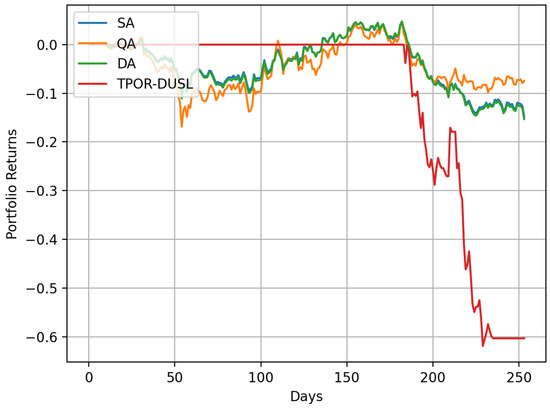
Figure 5.
Portfolio performance with optimization weights in the year 2020.
In the above experiments, we observed that the created portfolios used between 80 and 120% of the available capital. Thus, sometimes we observed overspending and sometimes underspending. Although this is not a big problem in our approach, as we can just keep the proportions and scale the whole portfolio such that exactly 100% of the capital is used, we still can enforce this constraint by increasing the parameter . To investigate the effect of increasing in our QUBO model, we examined the results of Figure 3 with respect to the capital spent in the created portfolios. In the experiments visualized in Figure 3, we observed that the portfolios created by simulated annealing and digital annealing already used exactly 100% of the capital, while the portfolios created by quantum annealing were off by approximately ±9%. When increasing the value of from 1 to 100, we get the results as seen in Figure 6.
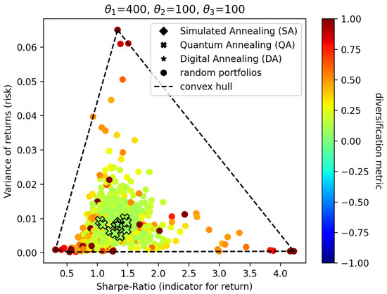
Figure 6.
Annealing results with increased weight on the budget.
An interesting result when comparing Figure 6 with the previous experiments of Figure 3 is that when increasing , portfolios with a lower Sharpe ratio seemed to be created. For the portfolios created by simulated annealing and digital annealing, we observed that all the created portfolios used % of the whole capital. The increase of did not show any significant impact on portfolios created by quantum annealing. Here, we still observed that the portfolios used ±10% too much (or too little) of the budget.
8. Conclusions
In this paper, we have introduced a new workflow to solve portfolio optimization problems. We have started with a classical preprocessing step in which we used classical backtesting for all pairs-trading and trend-following strategies. We applied the strategies to historical real-world data within the time span of 2015–2019. Based upon the results of this step, we chose the most promising strategy/asset combinations as an input to our modified QUBO formulation for portfolio optimization. Our modified QUBO model enables an investor to place an arbitrary amount into arbitrary many assets. The solutions to our QUBO formulation create portfolios in which a certain fraction of the overall budget is dedicated to certain strategies, while also respecting the amount of risk that should be taken and the magnitude of return that should be achieved. We evaluated our QUBO formulation via simulated annealing, digital annealing, and quantum annealing. The simulated annealing results show that our approach works as intended, meaning that portfolios were generated that respect the given preferences of the investor (expressed by the chosen values of ) while also creating diversified portfolios. The results of quantum annealing were also promising, yet not as good as the simulated annealing and digital annealing results. The probable cause for this is a combination of inherent noise, missing error correction, scaling of the parameters, and others. We note, however, that we only used default parameters for all of our evaluations. Hence, for future work, finding and using more suitable parameter configurations or adding techniques such as reverse annealing or certain types of low polynomial running-time post-processing might significantly increase solution quality in all cases. The combination of classical algorithms and reverse annealing might also provide benefits over purely classical or purely quantum methods.
Author Contributions
Conceptualization, S.F. and J.L.; Methodology, J.L., S.Z. and S.F.; Software, J.L.; Validation, J.L., S.Z. and S.F.; Writing—original draft preparation, J.L.; Writing—review and editing, J.L., S.Z. and S.F.; Supervision, S.F. All authors have read and agreed to the published version of the manuscript.
Funding
This research received no external funding.
Institutional Review Board Statement
Not applicable.
Informed Consent Statement
Not applicable.
Data Availability Statement
Not applicable.
Conflicts of Interest
The authors declare no conflict of interest.
References
- Shor, P.W. Algorithms for quantum computation: Discrete logarithms and factoring. In Proceedings of the 35th Annual Symposium on Foundations of Computer Science, Santa Fe, NM, USA, 20–22 November 1994; pp. 124–134. [Google Scholar]
- Lucas, A. Ising formulations of many NP problems. Front. Phys. 2014, 2, 5. [Google Scholar] [CrossRef]
- Glover, F.; Kochenberger, G.; Du, Y. A tutorial on formulating and using QUBO models. arXiv 2018, arXiv:1811.11538. [Google Scholar]
- Ikeda, K.; Nakamura, Y.; Humble, T.S. Application of quantum annealing to nurse scheduling problem. Sci. Rep. 2019, 9, 12837. [Google Scholar] [CrossRef] [PubMed]
- Venturelli, D.; Kondratyev, A. Reverse quantum annealing approach to portfolio optimization problems. Quantum Mach. Intell. 2019, 1, 17–30. [Google Scholar] [CrossRef]
- Milne, A.; Rounds, M.; Goddard, P. Optimal Feature Selection in Credit Scoring and Classification Using a Quantum Annealer; 1QB Information Technologies: Vancouver, BC, Canada, 2017. [Google Scholar]
- Rosenberg, G. Finding Optimal Arbitrage Opportunities Using a Quantum Annealer; 1QB Information Technologies Write Paper; 1QBit: Vancouver, BC, Canada, 2016; pp. 1–7. [Google Scholar]
- Stollenwerk, T.; Lobe, E.; Jung, M. Flight gate assignment with a quantum annealer. In Proceedings of the International Workshop on Quantum Technology and Optimization Problems, Munich, Germany, 18–21 March 2019; Springer: Munich, Germany, 2019; pp. 99–110. [Google Scholar]
- Martoňák, R.; Santoro, G.E.; Tosatti, E. Quantum annealing of the traveling-salesman problem. Phys. Rev. E 2004, 70, 057701. [Google Scholar] [CrossRef]
- Neukart, F.; Compostella, G.; Seidel, C.; Von Dollen, D.; Yarkoni, S.; Parney, B. Traffic flow optimization using a quantum annealer. Front. ICT 2017, 4, 29. [Google Scholar] [CrossRef]
- Elsokkary, N.; Khan, F.S.; La Torre, D.; Humble, T.S.; Gottlieb, J. Financial Portfolio Management Using D-Wave Quantum Optimizer: The Case of Abu Dhabi Securities Exchange; Technical Report; Oak Ridge National Lab.(ORNL): Oak Ridge, TN, USA, 2017. [Google Scholar]
- Markowitz, H. Portfolio selection. J. Financ. 1952, 7, 77–91. [Google Scholar]
- Porth, L.; Pai, J.; Boyd, M. A portfolio optimization approach using combinatorics with a genetic algorithm for developing a reinsurance model. J. Risk Insur. 2015, 82, 687–713. [Google Scholar] [CrossRef]
- Xidonas, P.; Steuer, R.; Hassapis, C. Robust portfolio optimization: A categorized bibliographic review. Ann. Oper. Res. 2020, 292, 533–552. [Google Scholar] [CrossRef]
- Zhang, Z.; Zohren, S.; Roberts, S. Deep learning for portfolio optimization. J. Financ. Data Sci. 2020, 2, 8–20. [Google Scholar] [CrossRef]
- Marzec, M. Portfolio optimization: Applications in quantum computing. In Handbook of High-Frequency Trading and Modeling in Finance; John Wiley & Sons: Hoboken, NJ, USA, 2016; pp. 73–106. [Google Scholar]
- How Quantum Computing Could Change Financial Services. Available online: https://www.mckinsey.com/industries/financial-services/our-insights/how-quantum-computing-could-change-financial-services (accessed on 20 November 2022).
- Quantum Computing in Finance: Quantum Readiness for Commercial Deployment and Applications. Available online: https://services.global.ntt/-/media/ntt/global/insights/blog/the-new-world-of-banking/quantum-computing-whitepaper.pdf (accessed on 20 November 2022).
- Phillipson, F.; Bhatia, H.S. Portfolio Optimisation Using the D-Wave Quantum Annealer. arXiv 2020, arXiv:2012.01121. [Google Scholar]
- Cohen, J.; Khan, A.; Alexander, C. Portfolio Optimization of 40 Stocks Using the DWave Quantum Annealer. arXiv 2020, arXiv:2007.01430. [Google Scholar]
- Cohen, J.; Khan, A.; Alexander, C. Portfolio Optimization of 60 Stocks Using Classical and Quantum Algorithms. arXiv 2020, arXiv:2008.08669. [Google Scholar]
- Narang, R.K. Inside the Black Box: A Simple Guide to Quantitative and High Frequency Trading; John Wiley & Sons: Hoboken, NJ, USA, 2013; Volume 846. [Google Scholar]
- Chan, E. Quantitative Trading: How to Build Your Own Algorithmic Trading Business; John Wiley & Sons: Hoboken, NJ, USA, 2009; Volume 430. [Google Scholar]
- Chan, E. Algorithmic Trading: Winning Strategies and Their Rationale; John Wiley & Sons: Hoboken, NJ, USA, 2013; Volume 625. [Google Scholar]
- Nikolaev, A.G.; Jacobson, S.H. Simulated annealing. In Handbook of Metaheuristics; Springer: New York, NY, USA, 2010; pp. 1–39. [Google Scholar]
- Kirkpatrick, S.; Gelatt, C.D.; Vecchi, M.P. Optimization by simulated annealing. Science 1983, 220, 671–680. [Google Scholar] [CrossRef] [PubMed]
- King, A.D.; McGeoch, C.C. Algorithm engineering for a quantum annealing platform. arXiv 2014, arXiv:1410.2628. [Google Scholar]
- Matsubara, S.; Takatsu, M.; Miyazawa, T.; Shibasaki, T.; Watanabe, Y.; Takemoto, K.; Tamura, H. Digital annealer for high-speed solving of combinatorial optimization problems and its applications. In Proceedings of the 2020 25th Asia and South Pacific Design Automation Conference (ASP-DAC), Beijing, China, 13–16 January 2020; pp. 667–672. [Google Scholar]
- King, J.; Yarkoni, S.; Raymond, J.; Ozfidan, I.; King, A.D.; Nevisi, M.M.; Hilton, J.P.; McGeoch, C.C. Quantum annealing amid local ruggedness and global frustration. J. Phys. Soc. Jpn. 2019, 88, 061007. [Google Scholar] [CrossRef]
- Albash, T.; Lidar, D.A. Demonstration of a scaling advantage for a quantum annealer over simulated annealing. Phys. Rev. X 2018, 8, 031016. [Google Scholar] [CrossRef]
- Tsukamoto, S.; Takatsu, M.; Matsubara, S.; Tamura, H. An accelerator architecture for combinatorial optimization problems. Fujitsu Sci. Tech. J 2017, 53, 8–13. [Google Scholar]
- Farhi, E.; Goldstone, J.; Gutmann, S. A quantum approximate optimization algorithm. arXiv 2014, arXiv:1411.4028. [Google Scholar]
- Lewis, M.; Glover, F. Quadratic unconstrained binary optimization problem preprocessing: Theory and empirical analysis. Networks 2017, 70, 79–97. [Google Scholar] [CrossRef]
- Fang, Y.; Lai, K.K.; Wang, S. Fuzzy Portfolio Optimization: Theory and Methods; Springer Science & Business Media: Berlin, Germany, 2008; Volume 609. [Google Scholar]
- Rebentrost, P.; Lloyd, S. Quantum computational finance: Quantum algorithm for portfolio optimization. arXiv 2018, arXiv:1811.03975. [Google Scholar]
- Palmer, S.; Sahin, S.; Hernandez, R.; Mugel, S.; Orus, R. Quantum portfolio optimization with investment bands and target volatility. arXiv 2021, arXiv:2106.06735. [Google Scholar]
- Ottaviani, D.; Amendola, A. Low rank non-negative matrix factorization with d-wave 2000q. arXiv 2018, arXiv:1808.08721. [Google Scholar]
- Gabor, T.; Zielinski, S.; Roch, C.; Feld, S.; Linnhoff-Popien, C. The UQ Platform: A Unifed Approach To Q uantum Annealing. In Proceedings of the 2020 5th International Conference on Computer and Communication Systems (ICCCS), Shanghai, China, 15–18 May 2020; pp. 115–119. [Google Scholar]


Publisher’s Note: MDPI stays neutral with regard to jurisdictional claims in published maps and institutional affiliations. |
© 2022 by the authors. Licensee MDPI, Basel, Switzerland. This article is an open access article distributed under the terms and conditions of the Creative Commons Attribution (CC BY) license (https://creativecommons.org/licenses/by/4.0/).