Abstract
Experimental crude datasets are usually processed with statistical methods to obtain rough evaluations of nautical measurements. Taking the observations and rectifying the knowledge on them are not correlated. In modern computer applications, raw datasets are usually exploited in the initial learning phase. At this stage, the available data are explored to extract the necessary parameters required within the scheme of computations. The aim of this study was to undertake the crude data processing problem to extract the conditional dependencies that appear as the most important factors when handling the distorted data. First, I upgraded the traditional structures, which are histograms. The stepwise diagrams feature their uncertain evaluation. I upgraded the hierarchy among the evidence within the data pool and defined the given ranking adequate membership functions. The principles of fuzzy systems justified the use of the bin-to-bin additive approach to obtain the locally injective density functions, which can be perceived of as conditional dependency diagrams that enable the construction of simple belief assignments. The structural combination includes the solution to the position fixing problem.
1. Introduction
Dealing with imprecise data requires models that include knowledge in the framework. To meet this requirement, one should engage fuzzy systems and the mathematical theory of evidence (MTE), which deliver platforms for processing uncertainty [1,2,3]. The models require methods for obtaining formal evaluations of the uncertainty. In nautical science, the knowledge refers to the distribution of the random variable instances, which are usually perceived of as governed by Gaussian dispersion patterns. Knowing the magnitude of the standard deviations enables the introduction of a rough assessment observation in terms of good, bad, or sufficient, which is an approach that is popular among specialists. For those who are involved in implementing computer procedures, a variety of measurement qualities are perceived of as uncertainty and should be included in the processing scheme. The author of [4] discuss this concept, proposing a model of accepted nautical knowledge thanks to evidence proximity exploration and the engagement of the principles of fuzzy systems. Based on the available navigation systems, the author defined the standard deviation adequate membership functions and input them into the processing. In the proposed approach, analyses of the available raw recorded instances are performed to extract an even wider range of useful parameters. The author proposes the scope and methods of their evaluation. Thanks to this model, the prior estimations are of secondary meaning and do not directly affect the final solutions. However, the former evaluations might be unavailable; thus, the suggested approach appears as a universal one whenever random data are involved. Moreover, the evidence engaged in the problem should be normalized, and the decisiveness in terms of the effect of the solution should be ranked. Items with lower uncertainty have the most substantial influence in this respect. This paper contains a section that is devoted to defining the hierarchy among the evidence within a pool of data.
The proposed approach engages fuzzy sets and the combination mechanism available in the MTE [4]. I suggest and describe the necessary conversions and transformations of the traditional histograms. In this respect, the paper is an extension of the previous one delivered by the author of [5]. I describe uncertain data handling, histogram transformation, and their applications for solving the object identification problem. The expansion aims at the conditional dependency excavation from the recorded instances of distorted variables. I use the position fixing problem as an example to implement the presented idea.
2. Understanding Position Fixing
Making a fix is an inference scheme that involves evidence and hypotheses [6,7]. One can reason as to the particular location of the truth that represents the observer’s position given all the available observations, as well as to the knowledge regarding each of them [8].
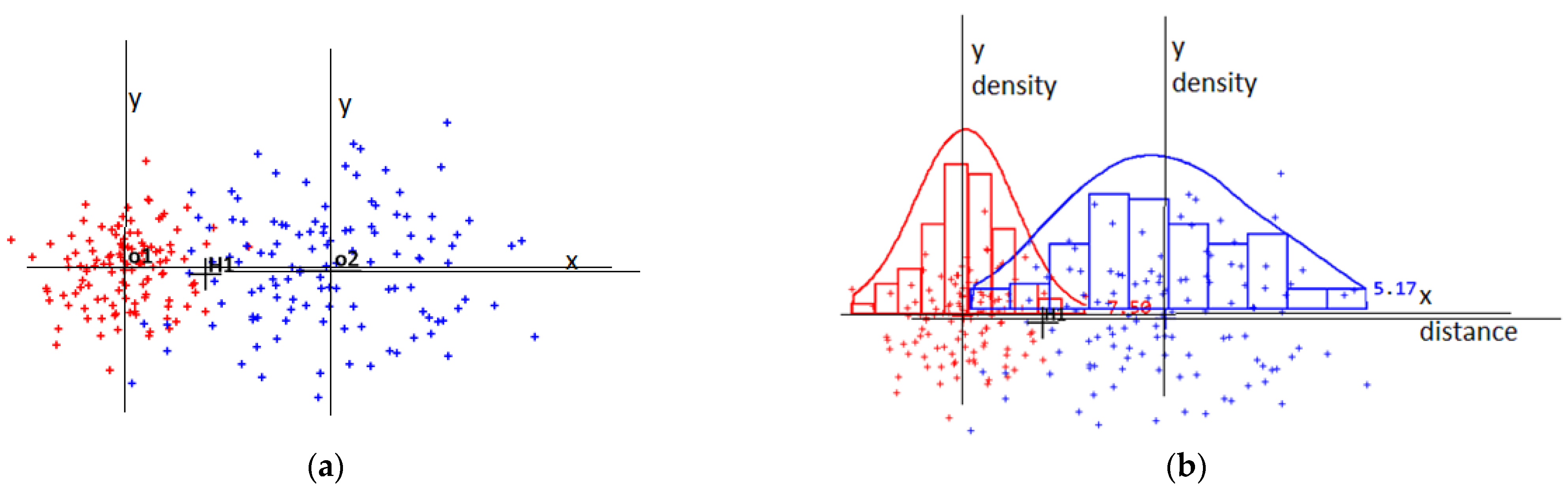
I illustrate the idea in Figure 1a, in which I display two pieces of evidence (o1 and o2), with the sets of instances indicating their dispersions. I also present the single-hypothesis point labelled H1. The statement that a given location (H1) is the true position gains some support from each piece of available evidence. I assumed that the involved data were diversified regarding their quality. For the situation presented in Figure 1, Observation o1 seems to be more reliable than Observation o2. The density of the instances that fall close to o1 is greater than that of the ones that fall close to o2.
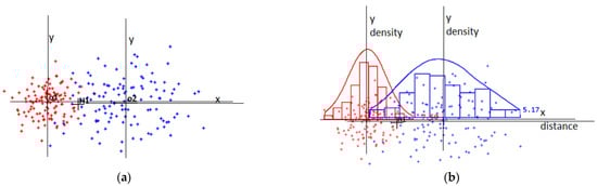
Figure 1.
(a) Two observations with examples of their dispersions and single-hypothesis locations; (b) horizontal-axis distributions converted to histograms and their continuous versions.
I present the results of the processing, including the instance sets, in Figure 1b. Statistical evaluations of the example system indications are missing. Instead, I converted the raw data to histograms, which I further transformed to injective diagrams of the density functions. Local injection is required to obtain solutions for many problems that engage random variables [9]. I present the basic scheme followed during the position fixing and imprecise data handling in Figure 1. The general pattern of the presented rational also fits the arrangement.
In order to calculate the support measure of the truth that a point represents the true location, we need to define and solve the partially related tasks, evaluate the trustworthiness of the observations at hand, and propose the methodology of the support estimation included in each observation. Taking advantage of fuzzy sets and Bayesian conditional dependencies enables an adequate approach proposal. Finally, we need to upgrade the basic probability assignments and their combinations. The results of the conjunctive associations embed the sought support measures.
Researchers have performed many studies on the modified concept of random data handling [10], which represents a shift towards the discrete space of solutions and the mathematical theory of evidence as the basic platforms of processing schemes. The broad scope of consequences includes the verified approach to the meaning of the accuracy. A natural feature of the new approach is the ability to evaluate the truth attributed to the obtained solutions. A supporting measure of a ship’s fixed location at a particular position is embedded in the processing scheme. Most researchers start from statistical evaluations of the random instance behaviour, and they often encounter Gaussian distributions. The included uncertainty usually refers to a variety of available standard deviations. Self-contained modern applications should contain initial data processing modules. Their lifecycles should contain a learning phase, while the raw input data should be analysed to mine the necessary initial items.
Bayesian conditional dependencies deliver a unique opportunity to evaluate the hypothesis truth based on the related evidence at hand. In nautical science, observations and the linked knowledge are the main constituents of the evidence. The widely known information on the taken observation represents an instance of random variables, and usually sets of samples are available. The data distribution functions need to be identified to render the sets useful. Attempts to consider the Gaussian functions as density patterns dominated in the traditional approach. However, raw sets are forgotten and statistical measures, such as standard deviations and elliptic or circular errors, are used instead. The informative context of the initial raw data is rather rich; thus, the method of using them should be reconsidered. In this paper, I present a revised approach to the exploitation of unprocessed data. The measures that represent the true location of any point in the neighbourhood of the observation are the conditional dependency values, which are written as and are considered as a measure of support for the hypothesis (xi) that is embedded within the observation (oj). Random data processing contains three steps: (1) the learning phase, in which the raw experimental data are gathered and recorded; (2) the upgrading of the x- and y-axis histograms; (3) the evaluation of the empirical data structures to extract the embedded uncertainty, which is the main factor to consider when obtaining the converted forms of stepwise density functions. To achieve unique solutions, the density functions should be injective ones, and to guarantee this, I propose the injective function transformation of histograms. The fuzzy-set concept is helpful for the conversion from the empirical form of the probability density.
In the traditional approach, the modelling and processing of imprecise data are impaired. Moreover, the results of the observations and their quality evaluation can be achieved prior to the measurements being taken. The a posteriori analysis is compromised and is not embedded into the scheme of the traditional manner of inaccurate data handling. In the new solutions, one starts with an alternative approach to doubtfulness modelling. Fuzzy density sets are established around each of the nautical indications. The concept should be taken into consideration once the most probable measurement location has been detected, the position fixing has been performed, and the systematic error has been identified.
The presented rational refers to the evidence and hypothesis scheme of reasoning that are encountered in nautical practice and science. No measurement or indication read from a nautical aid is exact. When a quantity is measured or indicated, the outcome depends on the aid or the involved system precision. The measurement environment conditions, as well as the skill of the observer, are also important. Thus, the available pieces of evidence support hypothesis items with different factors. The higher-quality data should more decisively contribute to the hypothesis truth. In the case of position fixing, the nautical quantity magnitude of the uncertainty should affect the final solution. Less uncertain measurements and/or indications have a greater effect on the selection of the true location. Therefore, the evaluation of the random variable instances is important, and it starts from an analysis of the experiments that involve the observations of the instances given an indication.
3. Random Data Processing
The distributions of the two-dimensional indications of the approximately observed locations are subjected to processing to obtain knowledge on the accuracy of the available navigational aids. Such processing is rarely performed in computer-based applications. Currently, seafarers exploit the standard deviations of Gaussian functions as satisfactory substitutes that fulfil the popular practical nautical requirement with regard to the uncertainty evaluation, and the statistical dispersions are important factors. Seafarers only consider the delivered indication to be complete when it is accompanied by a specification of the associated uncertainty, which is usually understood as the circular or elliptic deflection. The values reflect the quality of the delivered data.
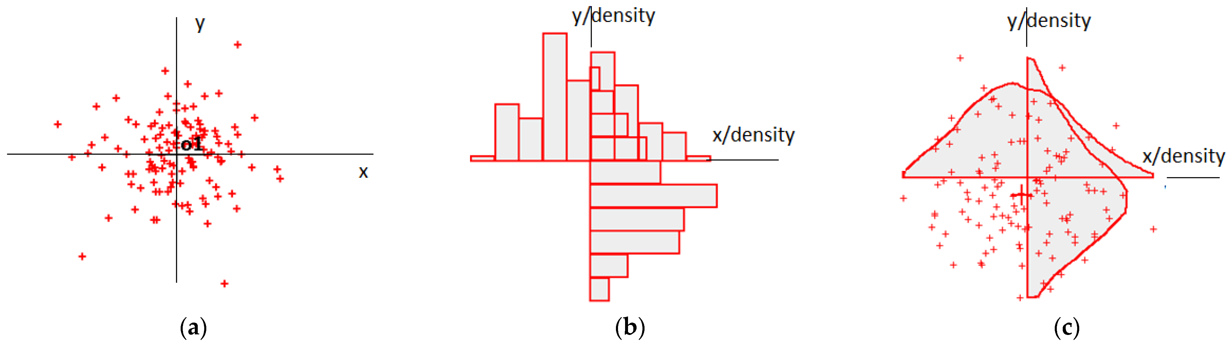
I present the steps of the proposed random two-dimensional data processing in Figure 2. In the left part, I present the raw experimental data as the output of the various recorded experiments. I further upgraded the x- and y-axis histograms, and I evaluated the empirical data structures according to the embedded uncertainty. The doubtfulness is the main factor to consider when obtaining the converted forms of stepwise density functions. To achieve unique solutions, the density functions should be locally injective ones.
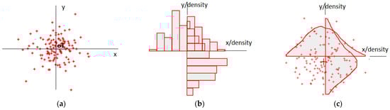
Figure 2.
(a) Instance of observation with its distribution set; (b) horizontal- and vertical-axis histograms; (c) horizontal- and vertical-axis converted histograms.
The goal of the illustrated processing scheme is the creation of a function, converted histogram. The locally injective diagram enables the establishment of a conditional relationship (). The latter is a measure of the support for a given hypothesis, which is an element of the set (X) that is embedded within a particular observation that belongs to the collection (O).
4. Random Data Evaluation
In random data evaluation, the aim is at the discovery of certain patterns included within the available sets of their instances. Upgrading histograms is usually the first step of the analyses. A histogram consists of bins or cells that are represented as adjacent rectangles. The histogram displays the proportion of cases that fall into each bin. Although histograms are popular and widely used, attempts to judge or calculate their quality or value are rather scarce.
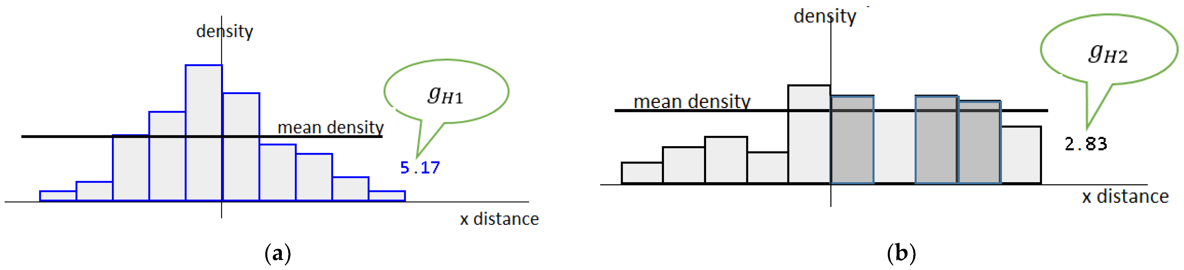
Histograms should be subjected to either intuitive or objective evaluation. The MTE, with its probability assignments, stipulates their impartial evaluation. The differentiations refer to their bin heights and ranges, as well as to the structure expansion. The uncertainty refers to a certain feature within the discussed scope that is considered constant within a particular domain. The number of items with the same or almost the same value of the feature defines the uncertainty. In this view, the uncertainty is related to the distinguishability. There are more indistinguishable abscissa points presented in Histogram (b) of Figure 3 than in Histogram (a) (see depicted bins in the right part of the figure). Thus, Histogram (a) contains a less amount of uncertainty than Histogram (b). We can use the diversity in the bin heights as a factor to measure the distinguishability. The average number of cases that fall below and above the horizontal central line of a histogram is the objective measure of the bin diversity. The inserted numbers in Figure 3 are the respective metrics for the presented cases. The greater the figure, the “better” the histogram. The total of all the points that fall above and below the presented horizontal line may be zero when there is a uniform distribution of the feature, which is in line with the popular understanding of uncertainty. We can perceive of doubtfulness as the thinking that something might be somewhere within a given scope, but there is no hint as to where. A histogram with the same cell heights is extremely unreliable. The total of the instances below and above the central line is zero.
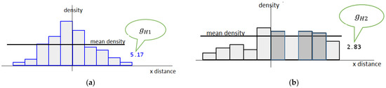
Figure 3.
Interpretation of histogram uncertainty with respect to bin heights: (a) better-shaped histogram; (b) worse-shaped histogram.
Relative rather than absolute uncertainty is often of primary importance. Position fixing is an example of a problem in which the relativity of the uncertainties really matters. The idea is to establish the grades that affect the final solution by each piece of evidence compared with other ones. The relative weight of the contribution to the final solution is an important issue. Given a set of histograms and the range and bin height for each structure, we can calculate the adequate measures. We can obtain the relative deflection and result uncertainty attributed to the i-th structure with the following formula:
where is the maximum bin height measure for the histograms involved, calculated as the average number of cases that fall below and above the medium value, and the following holds: (the greater the value, the more diversified the histogram) (see Figure 3 for illustration); is the bin height measure for the i-th histogram; is the subjectively valued minimal uncertainty regarding the bin height measure for the histograms involved.
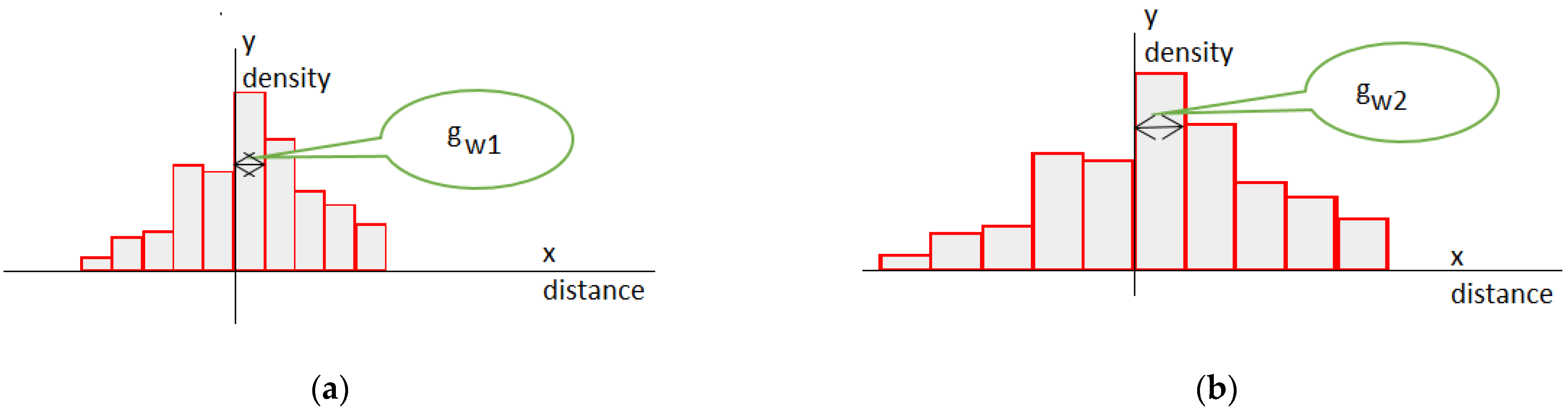
As mentioned above, the number of items with features of the same value defines the uncertainty. Thus, considering two histograms with the same numbers of bins and different bin widths, one can assume that the wider structure embeds greater uncertainty. Histogram (a) in Figure 4 contains a smaller amount of uncertainty than Histogram (b).
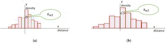
Figure 4.
Interpretation of histogram uncertainty with respect to bin widths: (a) better-quality histogram; (b) worse-quality histogram.
Given a set of histograms with various bin widths, we can calculate the relative deflection and result uncertainty using the following expression:
where is the minimum bin width for the histograms involved, and the denominator of Equation (2) is assumed to be greater than zero (see Figure 4 for illustration); is the bin width measure for the i-th histogram; is the subjectively valued minimal uncertainty regarding the bin width measure for the histograms involved.
Given the independent uncertainties related to the diversity of the bin heights and widths, one can obtain the resulting histogram uncertainty () from Equation (3):
The presented equations engage the features of two structures. In the case of the exploitation of data pools that contain multiple sets, the initial reference histogram is necessary to create the required hierarchy. The histogram may take the shape of a logical structure that enables the obtainment of the proper relations within the considered pool. The sorted uncertainty list ({ΘRi ≤ ΘRi+1}) indicates a hierarchy in the available evidence, and it needs to be upgraded to obtain the correct solution. The first item on the list contains the smallest uncertainty, and its evaluation requires recalling the elements of a hypothetical structure. The initial structure () with a set of attributes ({,,}) is created to obtain the required ranking.
The components in the logical ideal structure () are as follows:
: the best bin height measure for a given set of histograms;
: the best bin width measure for a given set of histograms;
: the default reference bin height for the basic uncertainty measure;
: the default reference bin width for the basic uncertainty measure.
The proposed ideal histogram is a logical structure that is upgraded for a particular data pool. The reference bin height and width measures for a given set of histograms are selected. The histogram is a collection of the best options established based on the considered dataset. Because there is no histogram without uncertainty, a default value is assigned. Hereafter, the included examples exploit 0.05 as the basic bin height uncertainty, and 0.1 as the minimal width uncertainty.
5. Histogram Transformation
A histogram displays a stepwise diagram of the distribution of the observed data. A histogram consists of adjacent rectangles that are primarily erected over nonoverlapping intervals. The histogram displays the relative frequencies, which are the empirical probabilities, and it shows the proportion of cases that fall into each bin. The problems that arise when using raw experimental data that are intended for the nautical scope of applications are as follows:
- How to evaluate the histograms;
- How to convert the stepwise diagram to take the form of the locally injective function;
- How to prepare a family of histograms for use when solving a particular problem (for example, position fixing).
The exploration of a histogram layout results in its evaluation. The vertical and horizontal features are the bases for the judgement of the quality of the involved samples of the random data instances.
Combining assignments that engage density data generates adequate and useful solutions once the injective concentration functions, or at least the locally injective concentration functions, are processed. However, we should not expect unique solutions when traditional histograms are involved. Converting the rectangular bins to fuzzy density sets changes the overall image of the histogram. A stepwise diagram might take the form of a continuous locally injective function, which consequently enables researchers to solve many practical problems with imprecise data. To obtain a new version of the histogram, we have to consider that, to some extent, a single discernment point belongs to each considered bin when treating them as fuzzy sets. Instead of a rectangular-shaped bin, an area limited by the membership function (MF) is considered.
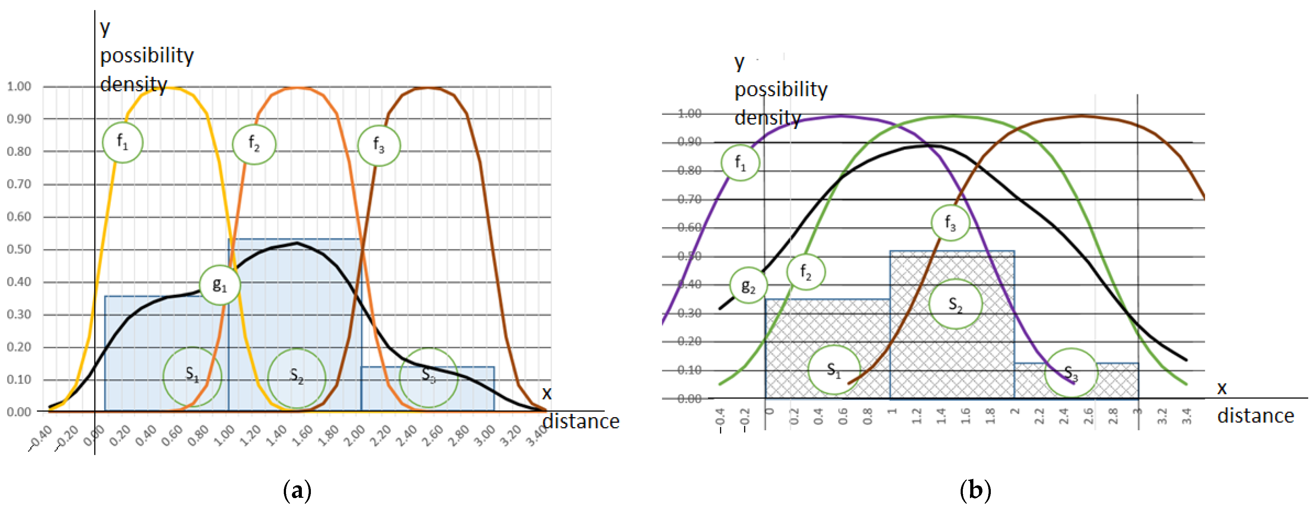
An inclusion diagram should feature some expectations to fulfil the equivalency requirements. The integral of a product of the belonging grades, and given the cell density, must be the same as the original bin’s area (see Equation (5)), and its vertex should be in the middle of the cell. The value that it returns at the left and right limits of the reference uncertainty area should be 0.5. In the simplest case, the uncertainty range is equivalent to the bin’s width. According to Equation (3), the cell’s range () defines only one part of the histogram uncertainty. Another compound is related to the irregularity of the cell heights. Thus, the MF that reflects the uncertainty extends beyond the cell limits. I present examples of the three membership diagrams in Figure 5. We can observe the previously mentioned items for the sigmoidal function pairs that define the borders of the cells for the three histograms. We can obtain the resulting neighbourhood density as the output of the additive combination of the same point inclusions within all the bins, as follows:
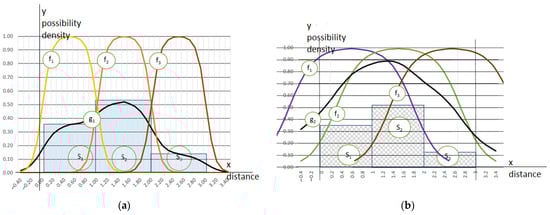
Figure 5.
Two examples of histograms, uncertainty-dependent membership functions, and transformed histograms. In the Si i-th histogram cell, the rectangular area showing the number of observations that fall within the range is assumed to be limited in terms of crisp values. fi is the membership function for the i-th cell, obtained for various uncertainty. gi is a continuous locally injective diagram of a modified histogram obtained for: (a) reasonable-quality data; (b) a worse-quality case.
Equation (4) presents the idea of the bin-to-bin additive concept that is crucial for the approach, where is the modified histogram, which is a density function for the l-th fragment of evidence; is the membership function, which is a grade of the xl inclusion in the i-th bin meant as a fuzzy set; n is the number of cells; is the height of the i-th cell.
I present diagrams of the membership functions for the three bin histograms with the different uncertainty levels regarding each case in Figure 5. The total of the membership grades for each of the points uniformly distributed over a considered space multiplied by the bin densities results in the cumulated belonging. The value is a plausibility measure that results in the modified histograms in Figure 5. The MF reaches a value of 1 in the middle of a bin, and it might return values of 0.5 at the cell’s limits (see the left presented case). Because the function should respond to the uncertainty that is included within the histogram, its scope is likely to extend beyond the cell’s limits (see the right part of Figure 5). The wider the expansion of the MF, the greater and less differentiated the calculated total membership, and the higher the diagram height of the modified histogram (compare Histograms (a) and (b) of Figure 5).
6. Membership Functions and Uncertainty
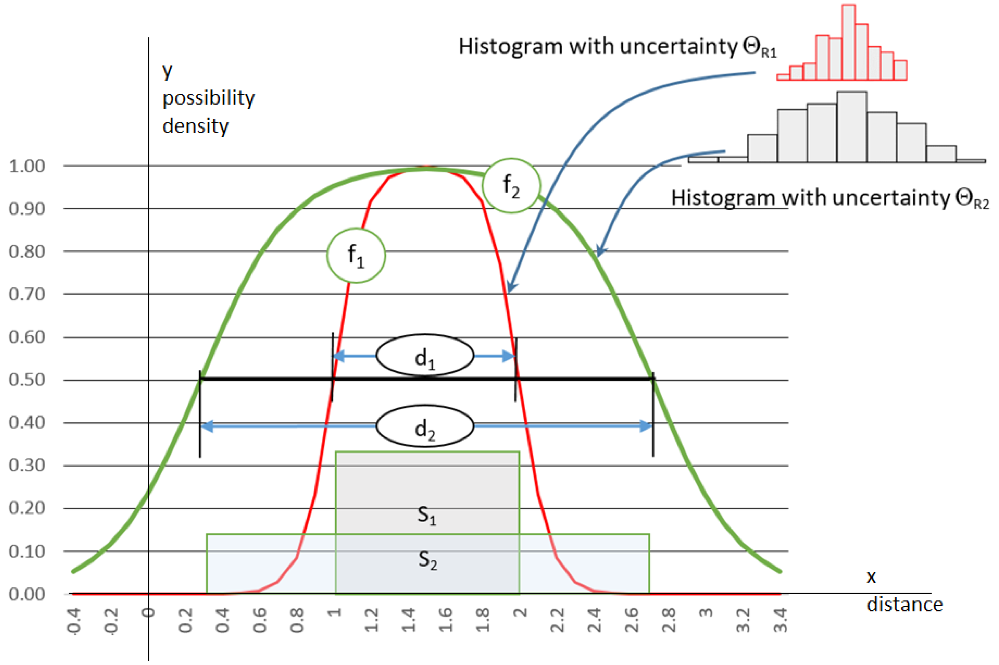
Equation (4) specifies the conversion of histograms featuring uncertainty. In the simplest case, the doubt is related to the histogram cell widths. As previously mentioned, the vertical variety of the cells also contributes to the overall uncertainty. Structures with the same cell heights are extremely unreliable. The case is rare, but it should be considered during analyses. In this situation, the resulting MF should take the form of a straight line that is parallel to the x-axis. In most practical cases, one can operate with α-cuts (assuming α equals 0.5) as the basic feature of the membership diagram. I present the basic issues that are important in the discussed field in Figure 6, which contains two histograms and uncertainty-dependent functions that reference the doubt in the cells of the inserted structural features (ΘR1 and ΘR2). The figure also includes the alpha-cut range.
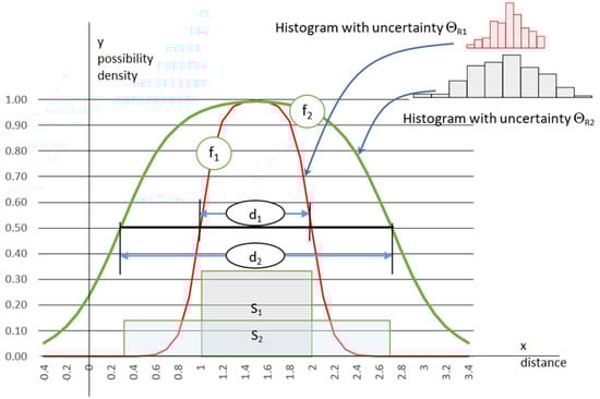
Figure 6.
Uncertainty-dependent membership functions for example case, where ΘR2 > ΘR1. fi is the membership function for the Si set feature of the i-th uncertainty level; di is the width of the 0.5 cut for the i-th membership function; Si is the underlying crisp limited histogram of the i-th cell.
The expansions of the function diagram are correlated with the uncertainty. Greater doubt means a wider MF range. The credibility of the evidence increases once its membership is closer to the singleton. According to the fuzzy-system-principle equation:
which is valid and can be used to derive the next expression:
Equation (6) expresses one of the most practical aspects of the introduced concept of the exploitation of the histogram uncertainty. Given the referential fuzzy object with its doubtfulness and MF range, the uncertainty attributed to the related structure allows us to deduce its membership diagram expansion.
7. Normalizing the Pool of Data
The position fixing problem exploits the collection of various quality observations, which need to be processed prior to the final usage. Preparing a pool of data requires their normalization to achieve uniform probability density distributions. Adequate conditional dependency functions need to be created. Moreover, the relative uncertainty vector enables definitions of the basic probability assignments. Fixing aims at the selection of a point that represents the true location of a ship in the optimal way. An evidence fragment supports the choice of each item from the considered set of hypotheses. The degrees of support are expressed as the conditional dependability, which relies on the credibility attributed to the evidence items. The items with low uncertainty should more decisively contribute to the selection. To implement the idea, we need to create a hierarchy ({ΘRi}) for the available evidence.
Table 1 contains the selected features for the example pools of the three indications. The recorded instances for each observation enable the creation of structures named HMi. The first processing engages histograms with their uncertainty assessments. The evaluation is made with reference to the HMref, the attributes of which are presented in the last piece of raw piece in Table 1. The assessments of the HM1 and HM2 are recalculated with respect to the best third observation. The final ranking list regarding the amount of uncertainty for this poll is {ΘR3, ΘR1, ΘR2}. The ranges of the membership functions are gathered in the last column labelled . These MFs are important uncertainty-dependent characteristics when obtaining the conditional dependencies, and they are necessary for the verification of hypotheses on the representation of the fixed position.

Table 1.
Selected features of example pools of three histograms.
The data presented above enable us to define a membership function as specified by Equation (7). The formula and bin-to-bin additive method lead to the modified diagrams, which can be perceived of as conditional dependency functions:
where xic is the mean of the i-th bin; is the leftmost limit of the i-th bin; is the rightmost limit of the i-th bin; ai is the steepness of the sigmoidal membership function.
The probability assignment consists of a pair of figures:
The probability assignment engages the j-th piece of the two-dimensional evidence and the i-th hypothesis object with x and y attributes, and it takes the form of a two-element set that is called the simple belief assignment.
In Equation (8), C is a constant and is assumed to be equal to one, and it refers to the width of an area at approximately the i-th hypothesis point. Note that and are density functions: is the conditional dependency for the (attribute x in hypothesis object ) included in the evidence (j-th observation), and is the conditional dependency for the (attribute y in hypothesis object ) included in the oj evidence (j-th observation). is the uncertainty of the j-th two-dimensional piece of evidence.
The constituent a is the j-th indication support that the i-th point is a true position, and it is a product of the density function as a diagram of the converted (X and Y) histograms, as well as a unary constant that defines the scope of the assumed neighbourhood. Constituent b is the mass of uncertainty that is imbedded in the j-th observation. The sum of both elements (a and b), as specified by Equation (8), must not be greater than one. A proportional reduction in the excess amount is suggested if necessary. The combination of all the assignments that involve a given point and all the observations provides a supporting measure that the location represents the true position of the observer.
The presented rational enables us to evaluate the conditional dependencies ( and ) once we have obtained the nautical aid indication. We mine the knowledge on their distribution from the raw experimental datasets. The converted histograms gXi and gYi are the outcomes of the preliminary computation made for the two-dimensional dispersion. An adequate probability is the area in the vicinity of any point of discernment. The density function is used to estimate the probability of a unary range around a given location. To avoid misunderstandings in the results, one should keep the proposed assumption in mind.
8. Application Example
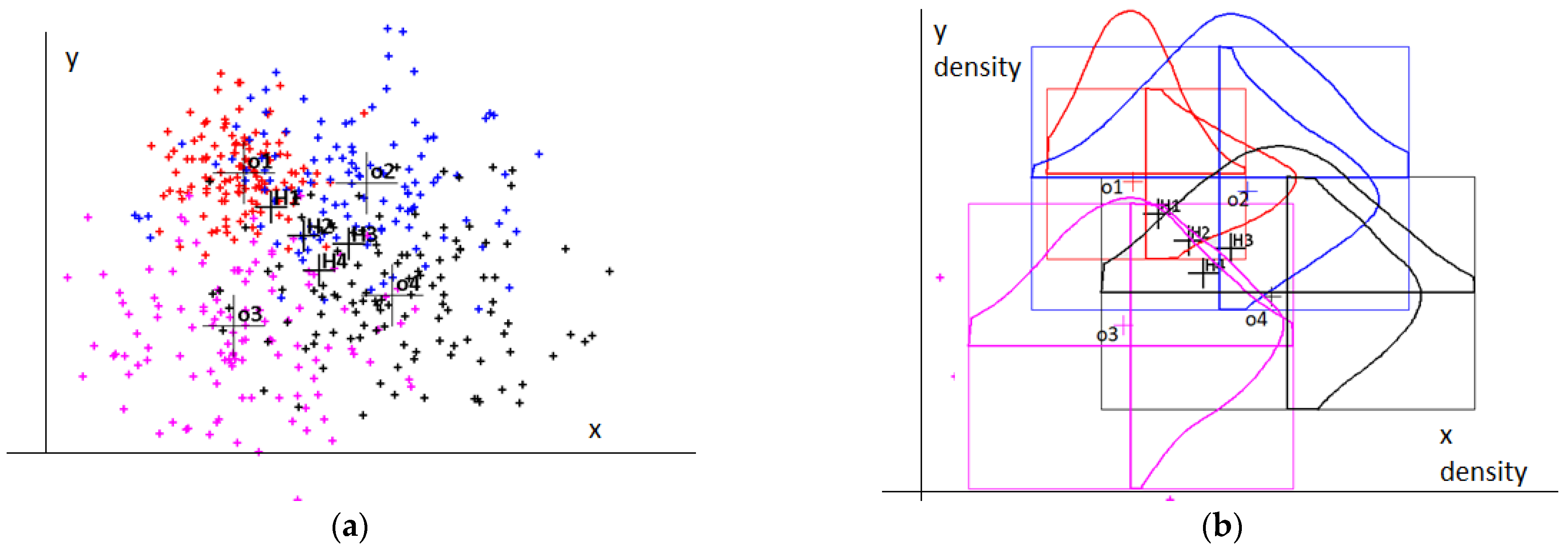
I present four pieces of evidence with four hypothesis points in Figure 7. I present the raw data on the left side of the illustration. On the right side, I present their converted probability density diagrams. I also present illustrations of the corresponding rectangles that cover the span of the raw datasets.
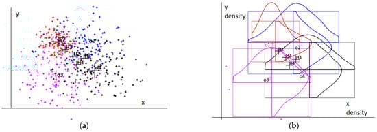
Figure 7.
Four pieces of evidence with four hypothesis points (oi is the i-th piece of evidence; Hi is the i-th hypothesis point): (a) evidence instance dispersions; (b) their converted histograms.
I present the conditional dependencies calculated based on those read from the diagrams in Table 2. For every hypothesis point, I obtained the belief assignments using Equation (8) by referring to each piece of evidence. The conjunctive combination of all the structures resulted in the cumulative measures. I present the final plausibility on the representation of a fixed position by each hypothesis point in the last column of the table. The first point represents the fix with the highest plausibility measure (0.472). The doubtfulness of the statement is close to zero. The last row of the table contains the relative uncertainties calculated for each piece of evidence. The best observation is o2, and it was used as the reference in the evaluation of the other uncertainties within the presented pool of observations.
Table 2.
Selected features for example pool of four histograms.
9. Conclusions
In this paper, I propose a new approach to imprecise data handling. I followed the inference computation scheme while the solving the fixed problem of the nautical solution. Raw experimental instances, which were available with statistically sufficient counts, were assumed to be the initial source of the knowledge regarding the behaviour of the available system indications. Modern applications include the learning phase, while the necessary elements are extracted for further usage. In the proposed approach, the conditional dependencies are discovered. The appropriate diagrams take the form of converted histograms, and they are constructed in one of the first processing steps. The evaluation of the construct reliability is an important issue. In this study, I considered the uncertainty regarding the vertical and horizontal layouts of the histogram. The measures refer to a variety of bin heights and widths, which enabled the estimation of the overall uncertainty. The doubtfulness and shape of the membership functions are mutually dependent. Both were main factors in the shape of the converted histograms, and they are the conditional dependencies in adequate diagrams. Making a fix is an example of the problem engaging distorted data, which requires additional processing. The normalization introduces uniform probability density distributions. The relative initial vector is constructed to obtain the required hierarchy and subsequent probability assignments. Their combination leads to the solution to the problem.
The proposed scheme for solving problems that involve distorted data includes several steps:
- The recording of the statistically justified number of instances for the involved sources of random data;
- An exploration of the stored sets to mine the embedded uncertainty. The suggested solution involves histograms, and I present a method for their evaluation in the paper;
- The creation of a ranking regarding the included doubtfulness within the available evidence items;
- The obtainment of locally injective density distribution diagrams and the consideration of them as conditional dependencies, given the uncertainty-dependent membership functions and bin-to-bin additive method;
- The use of the diagrams to upgrade the simple belief assignments of the MTE. The results of their associations include the measures that indicate the solution.
Funding
This research was funded by Gdynia Maritime University, Faculty of Management and Quality Science grant number WZNJ/2022/PZ/03. The APC was funded by WZNJ/2022/PZ/03.
Institutional Review Board Statement
Not applicable.
Informed Consent Statement
Not applicable.
Conflicts of Interest
The author declares no conflict of interest.
References
- Lee, E.S.; Zhu, Q. Fuzzy and Evidence Reasoning; Physica-Verlag: Heidelberg, Germany, 1995. [Google Scholar]
- Shafer, G. A Mathematical Theory of Evidence; Princeton University Press: Princeton, NJ, USA, 1976. [Google Scholar]
- Yen, J. Generalizing the Dempster—Shafer theory to fuzzy sets. IEEE Trans. Syst. Man Cybern. 1990, 20, 559–570. [Google Scholar] [CrossRef]
- Filipowicz, W. Mathematical Theory of Evidence in Navigation. In Belief Functions: Theory and Applications, Third International Conference; Cuzzolin, F., Ed.; Springer International Publishing: Cham, Switzerland, 2014; pp. 199–208. [Google Scholar]
- Filipowicz, W. Conditional dependencies in imprecise data handling. In Proceedings of the 25th International Conference on Knowledge-Based and Intelligent Information & Engineering, Szczecin, Poland, 8–10 September 2021. [Google Scholar]
- Dempster, A.P. A Generalization of Bayesian Inference; Springer: Berlin/Heidelberg, Germany, 2008; pp. 73–104. [Google Scholar]
- Denoeux, T. Allowing Imprecision in Belief Representation Using Fuzzy-valued Belief Structures. In Proceedings of the Information Processing and Management of Uncertainty in Knowledge-Based Systems, Paris, France, 6–10 July 1998. [Google Scholar]
- Filipowicz, W. A logical device for processing nautical data. Sci. J. Marit. Univ. Szczec. 2017, 52, 65–73. [Google Scholar]
- Filipowicz, W. Imprecise data handling with MTE. In Proceedings of the 11th International Conference on Computational Collective Intelligence, Hendaye, France, 4–6 September 2019. [Google Scholar]
- Yamada, K. Probability-possibility transformation based on evidence theory. In Proceedings of the Joint 9th IFSA World Congress and 20th NAFIPS International Conference, Vancouver, BC, Canada, 25–28 July 2001. [Google Scholar] [CrossRef]
Publisher’s Note: MDPI stays neutral with regard to jurisdictional claims in published maps and institutional affiliations. |
© 2022 by the author. Licensee MDPI, Basel, Switzerland. This article is an open access article distributed under the terms and conditions of the Creative Commons Attribution (CC BY) license (https://creativecommons.org/licenses/by/4.0/).