MFO Tunned SVR Models for Analyzing Dimensional Characteristics of Cracks Developed on Steam Generator Tubes

Abstract

Accurate prediction of material defects from the given images will avoid the major cause in industrial applications. In this work, a Support Vector Regression (SVR) model has been developed from the given Gray Level Co-occurrence Matrix (GLCM) features extracted from Magnetic Flux Leakage (MFL) images wherein the length, depth, and width of the images are considered response values from the given features data set, and a percentage of data has been considered for testing the SVR model. Four parameters like Kernel function, solver type, and validation scheme, and its value and % of testing data that affect the SVR model’s performance are considered to select the best SVR model. Six different kernel functions, and three different kinds of solvers are considered as two validation schemes, and 10% to 30% of the testing data set of different levels of the above parameters. The prediction accuracy of the SVR model is considered by simultaneously minimizing prediction measures of both Root Mean Square Error (RMSE), and Mean Absolute Error (MAE) and maximizing $R^2$ values. The Moth Flame Optimization (MFO) algorithm has been implemented to select the best SVR model and its four parameters based on the above conflict three prediction measures by converting multi-objectives into a single object using the Technique for Order of Preference by Similarity to Ideal Solution (TOPSIS) method. The performance of the MFO algorithm is compared statistically with the Dragon Fly Optimization Algorithm (DFO) and Particle Swarm Optimization Algorithm (PSO).

1. Introduction

Non-Destructive Testing (NDT) is a breakthrough in the industrial sector in the field of testing. Different components used in the industry need to be checked thoroughly for safety and better operability. Critical components such as SGTs and heater’s pressure values will be tested multiple times for their structural integrity to avoid damage while functioning; electromagnetic testing is also very useful in identifying the cracks in the SGTs and pipes. Daniel et al. [1] developed an ANN model to predict the SGT’s defect in terms of the length, width, and depth of crack from the given gray level co-occurrence matrix features from the Magnetic Flux Leakage (MFL) image. The structural integrity of the engineering components is increasingly very important in the modern scenario because of safety reasons. Usually, defects in steel pipes are cracks that might be in the surface or sub-surface; identifying any kind of such cracks and timely solving the issues will avoid a big disaster [2]. In NDT, different testing methods are available for each type of component or specimen needed to test. Normally, the NDT method will be determined based on the component/specimen size, shape, material, and conductivity of the material to be tested and the application capabilities of NDT techniques, including Visual Testing (VT), Ultrasonic Testing (UT), thermography, Radiographic Testing (RT), Electromagnetic Testing (ET), Acoustic Emission (AE), and shearography testing in terms of the benefits and drawbacks of these techniques. Based on their inherent qualities and applicability, further approaches are categorized. Most of the time, an NDT assessor simply employs one non-destructive test technique. Basic testing in NDT can be done with the expertise of individuals, but complex NDT testing requires experts with a wide knowledge of equipment operation and computer skills to obtain accurate results [3].

Material defects play a vital role in the industry, as they create major issues in the operation and safety of equipment and components. Material defects in the components and equipment can be inspected in two ways, like quality checking after manufacturing and on-site inspections during operations. Usually, most of the industry uses steel for the manufacturing of various equipment and components with different compositions, and steel will normally have defects like porosity, corrosion, pits, surface cracks, and sub-surface cracks, etc.; usually defects like corrosion, porosity, pits, and surface cracks can be manually identified with general NDT methods. The evaluation of the fracture area and the earlier identification of the cracks are particularly crucial, and those that are under stress or strain should be monitored regularly. Fatigue cracks or other pre-existing cracks may cause unexpected failure or disaster. Magnetic testing techniques produce good results in ferromagnetic materials and are extremely efficient for all components [4]. However, sub-surface cracks are difficult to find with the naked eye, and complex NDT methods should be used.

As a powerful and highly efficient non-destructive testing (NDT) method, magnetic flux leakage (MFL) testing is conducted based on the physical phenomenon that a ferromagnetic specimen in a certain magnetization state will produce magnetic flux leakage if any discontinuities are present in it. In the era of modern non-destructive testing, methods like magnetic flux leakage (MFL) testing have distinct benefits over conventional inspection techniques, including quicker inspection speeds, deeper examination depths, and simpler automated inspection. As a result, MFL testing is widely used in industries to evaluate ferromagnetic materials [5]. The specimen used during MFL experimental investigations of inner flaws or sub-surface fractures is often built with flaws that prevent the presentation of inner flaws of the same size but differing buried depths. A specimen with identical-sized interior flaws is conceived, built, and evaluated to study the MFL course of these defects. Identifying the sub-surface cracks also involves the simple magnetization of the material and obtaining the flux leakage output by using a hall sensor [6]. The periodic checking and verification of sub-surface cracks in critical areas may avoid drastic incidents. Magnetic flux testing (MFL) techniques are required in the inspection of steel tubes and pipes in the petrochemical industry, rope cars, nuclear reactor tubes, etc.

Ege and Coramik et al. [7] designed and produced two different PIGs to inspect pipelines using the flux leakage method. The authors also developed a new magnetic measurement system to investigate the effect of the speed variation of the produced PIGS. Shi et al. [8] introduced the principle, measuring methods, and quantitative analysis of the MFL method. The authors used statistical identification methods to establish the relationship between the defect shape parameter and magnetic flux leakage signals. Suresh et al. [9] developed a bobbin coil magnetizer arrangement to inspect the defects in small-diameter tubes and used an ANSYS Maxwell EM V-16-based Finite Element Method (FEM) and analytical model to support the experimental results.

For improving model accuracy, recently support vector regression (SVR), a machine learning tool, has gained focus among researchers in various fields to minimize prediction error. Jin et al. [10] proposed an internal crack-defect-detection method based on the relief algorithm and Adaboost-SVM, to overcome the problems of poor generalization and low accuracy in the existing defect detection process. Zhang et al. [11] developed an SVR regression model to forecast the stock price by optimizing the SVR parameters using dynamic adjustment and the opposition-based chaotic strategy in the Firefly Algorithm (FFA), termed the Modified Firefly Algorithm (MFFA). Kari et al. [12] implemented the SVR model with a Genetic Algorithm (GA) technique to forecast the dissolved gas content in power transformers to maintain the safety of the power system. Houssein et al. [13] used a twin support vector regression model to forecast the wind speed by tuning the SVR parameters by implementing the Particle Swarm Optimization (PSO) algorithm. Li et al. [14] presented a novel Sine Cosine Algorithm–SVR model to select the penalty and kernel function of SVR and validated the effectiveness by solving benchmark datasets. Yuvan et al. [15] introduced the GA–SVR model in forecasting sales volume to achieve better forecasting accuracy and performance than traditional SVR and Artificial Neural Network (ANN) prediction models. Pappadimitriou et al. [16] investigated the efficiency of the SVM forecasting model for the next-day directional change of electricity prices and reported 76.12% forecast accuracy over a 200-day period. Several other applications of SVR models exist in literature, ranging from process parameter prediction [17,18] to flow estimation [19] and from 3D-printing applications [20] to battery monitoring [21].

From the literature, it is understood that the SVR model, a machine learning tool, has been used by researchers in different areas like stock-market prediction, electricity prices, dissolved gas content, wind speed, etc. In this work, the SVR model is to be developed to predict the SGT’s defect in terms of length, width, and depth of cracks from the given gray level co-occurrence matrix feature from the Magnetic Flux Leakage (MFL) image. The selection of parameters, such as kernel function, solver type, and validation scheme, along with % of test data, will affect the performance of the SVR models. The root means square error, mean absolute error, and $R^2$ values are considered to measure the performance of the SVR model. Multiple contradictory performance measures require the conversion of multi-objectives into a single objective that initiated the implementation of the TOPSIS method. The Moth Flame Optimization Algorithm (MFO) is proposed to select the optimal parameters of SVR to minimize the prediction error. The effectiveness of the MFO algorithm is proven by comparing its performance with the Dragon Fly Optimization (DFO) and Particle Swarm Optimization (PSO) algorithms.

The paper is organized as follows. Section 2 describes the proposed methodology, SVR models, and MFO algorithm, along with its pseudocode and implementation. Section 3 deals with the results and discussion with a quantitative comparison of the performance of the MFO algorithm with the DFO and PSO algorithms. Finally, the conclusion part of the paper is given with future scope.

2. Machine Learning Methods

This paper proposes establishing a support vector regression model to predict the length, depth, and width of the given features of a crack image. The feature data set developed by Daniel et al. [1] is considered in this work to establish a more accurate SVR model compared to the neural network model. The data set had 22 features extracted from the 105 crack images with different lengths, depths, and widths. The model’s performance by different factors, such as kernel function, solver type, validation method and its parameters, and % of testing data set to validate the model are considered in this work. Built-in functions, such as ‘fitrsvm’ and ‘predict’, available in MATLAB 2022a version, have been used in this work to fit and predict the response value for the given training data set. The ‘resume’ function has been used to further train the SVR model until it reaches convergence status. Various performance measures are available; RMSE, MAE, and $R^2$ are considered in this work, MAE and $R^2$ are considered most often in literature and expressed in Equations (1)–(3). The above three performance measures will be calculated for the total data set, training data set, and testing data set separately and be considered for developing an optimized SVR model. Simultaneously minimizing both the values of RMSE and MAE and maximizing the $R^2$ values are taken as conflicting objectives, and a total of nine performance measures are involved; hence, the TOPSIS method is proposed in this work to convert these multi-objectives into a single objective using closeness values. Equations (4)–(9) are used to calculate the normalized value, performance matrix, the positive and negative ideal solution, ideal and negative ideal separation value, and closeness values, respectively. Figure 1 illustrates the proposed methodology of this work.

$$RMSE=\sqrt{\frac{{\sum }_{i=1}^{ns}{\left(R_{ik}-r_{ik}\right)}^2}{ns}}$$

(1)

$$MAE=\frac{{\sum }_{i=1}^{ns}\left|R_{ik}-r_{ik}\right|}{ns}$$

(2)

$$R^2=\frac{{\sum }_{i=1}^{ns}\left(R_{ik}-\overline{R_k}\right)\left(r_{ik}-\overline{r_k}\right)}{\sqrt{{\sum }_{i=1}^{ns}{\left(R_{ik}-\overline{R_k}\right)}^2{\sum }_{i=1}^{ns}{\left(r_{ik}-\overline{r_k}\right)}^2}}$$

(3)

where, $\overline{R_k}=\frac{{\sum }_{i=1}^{ns}{R}_{ik}}{ns}$ and $\overline{r_k}=\frac{{\sum }_{i=1}^{ns}{r}_{ik}}{ns}$

$$N_{rk}=\frac{O_{rk}}{\sqrt{{\sum }_{r=1}^{it}{O}_{rk}^2}}$$

(4)

$$A_{rk}=N_{rk}\ast W_k$$

Minimization:

$$P_k=\stackrel{\underset{it}{r=1}}{min}\left(A_{rk}\right)$$

$$M_k=\stackrel{\underset{m}{i=1}}{max}\left(A_{rk}\right)$$

(5)

Maximization:

$$P_k=\stackrel{\underset{it}{r=1}}{max}\left(A_{rk}\right)$$

$$M_k=\stackrel{\underset{it}{k=1}}{min}\left(A_{rk}\right)$$

(6)

$$S{P}_r=\sqrt{{\sum }_{k=1}^{nr}{(A_{rk}-P_k)}^2}$$

(7)

$$S{M}_r=\sqrt{{\sum }_{k=1}^{nr}{(A_{rk}-M_k)}^2}$$

(8)

$$R_r=\frac{S{M}_r}{S{P}_r+S{M}_r}$$

(9)

Figure 1. Proposed methodology.

Figure 1. Proposed methodology.

2.1. Support Vector Regression Model

The SVR model is adopted to compute the function relationship between independent (parameters—$P_{ij}$) and dependent (responses—$R_{ik}$) variables whose distributions are not known and concurrently minimize both model complexity and estimation errors. The model complexity and estimation errors are concurrently minimized by implementing SVR in the data set and its performance was outperformed compared to neural network models. A training SVR model used a training data set to learn about the data set and to construct a model about the generalization error by testing the model using an unseen data set. The response value is a function of multivariate parameters as represented in Equation (10), which can be written as Equation (11) to represent a linear regression support vector in terms of weight vector (W), a high dimensional space related to input parameter space, and a bias (b).

$$R_{ik}=f\left(P_{ij}\right)$$

(10)

where,

$P_{ij}$—jth Parameter of ith training data

$R_{ik}$—kth Response of ith training data

i—Index for training data (i = 1, 2, 3,…nt)

j—Index for parameter (j = 1, 2, 3,…np)

k—Index for response (k = 1, 2,3,…nr)

$$f\left(P_{ij}\right)=W\phi \left(P_{ij}\right)+b$$

(11)

The value of weight and bias is estimated by transferring the regression problem into the constraint minimization problem expressed in Equation (12).

$$minimize \frac{1}{2}\Vert W^2\Vert +C{\sum }_{i=1}^{nt}\left({\xi }_i+{\xi }_i^{*}\right)$$

(12)

where,

${\xi }_i$, ${\xi }_i^{*}$—lower and upper positive slack variables

$\frac{1}{2}\Vert W^2\Vert$—Flatness value of the function

$C\sum _{i=1}^{nt}\left({\xi }_i+{\xi }_i^{*}\right)$—Empirical error

C—Box constraint or penalty parameter value

Constraints:

$$R_{ik}-W\phi \left(P_{ij}\right)+b\le \epsilon +{\xi }_i^{*}$$

(13)

$$W\phi \left(P_{ij}\right)+b-R_{ik}\le \epsilon +{\xi }_i$$

(14)

$${\xi }_i,{\xi }_i^{*}\ge 0$$

(15)

where

$\epsilon$—Error tolerance

The constraint problem is resolved using the following Lagrange multiplier function as given in Equation (16), which should be minimized concerning the conditions mentioned in Equation (17). The list of parameters considered to establish an SVR model is presented in Table 1. A list of kernel functions and their formulas are depicted in Table 2.

$$f\left(P_{ij}\right)={\sum }_{i=1}^{nt}\left({\alpha }_{ij}-{\alpha }_{ij}^{*}\right) K(P_{ij}·P)+b$$

(16)

$$L\left(\alpha \right)=\frac{1}{2}{\sum }_{i,l=1}^{nt}\left({\alpha }_{ij}-{\alpha }_{ij}^{*}\right)\left({\alpha }_{lj}-{\alpha }_{ij}^{*}\right) K(P_{ij}·P_{lj})+\epsilon {\sum }_{i=1}^{nt}\left({\alpha }_{ij}^{*}+{\alpha }_{ij}\right)-R_{ij}{\sum }_{i=1}^{nt}\left({\alpha }_{ij}^{*}-{\alpha }_{ij}\right)$$

(17)

where

${\alpha }_{ij}^{*} \mathrm{and} {\alpha }_{ij}$—Non-negative Lagrange multipliers

$K\left(P_{ij}·P\right)$—Kernel function

Constraints:

$$\begin{array}{l}{\displaystyle \sum _{i=1}^{nt}}\left({\alpha }_{ij}^{*}-{\alpha }_{ij}\right)=0\\ 0\le {\alpha }_{ij}^{*}\le C\\ 0\le {\alpha }_{ij}\le C\end{array}$$

Table 1. List of parameters considered in SVR.

Parameters	Values
$\mathrm{Kernel} \mathrm{function} (k_f$)	Gaussian
	Radial basis function
	Polynomial
	Linear
	Quadratic
	Cubic
Solver (sr)	SMO (Sequential Minimal Optimization)
	ISDA (Iterative Single Data Algorithm)
	Q1LP (Quadratic Programming)
Validation scheme (vs)	Cross-validation Holdout validation
Validation scheme’s parameters	K-fold—Number of folds used for cross-validation (5 to 15) Holdout—% of data holdout for validation (10% to 40%)
% of training data	10% to 30%

Table 1. List of parameters considered in SVR.

Parameters	Values
$\mathrm{Kernel} \mathrm{function} (k_f$)	Gaussian
	Radial basis function
	Polynomial
	Linear
	Quadratic
	Cubic
Solver (sr)	SMO (Sequential Minimal Optimization)
	ISDA (Iterative Single Data Algorithm)
	Q1LP (Quadratic Programming)
Validation scheme (vs)	Cross-validation Holdout validation
Validation scheme’s parameters	K-fold—Number of folds used for cross-validation (5 to 15) Holdout—% of data holdout for validation (10% to 40%)
% of training data	10% to 30%

Table 2. Kernel functions and their formulas.

Kernel Function	Formula	Terms Used
Gaussian	$e^{-\left(\frac{{\Vert P_{ij}-P_{lj}\Vert }^2}{{\sigma }^2}\right)}$	$\Vert P_{ij}-P_{lj}\Vert$—Euclidean distance $\sigma$—Variance
Radial basis function	$e^{-\left(\gamma {\Vert P_{ij}-P_{lj}\Vert }^2\right)}$	$\gamma$—Scaler value
Polynomial	${\left(A+P_{ij}^T{P}_{lj}\right)}^n$	A—Free parameter n—Order of polynomial
Linear	$\left(P_{ij}^T{P}_{lj}\right)$
Quadratic	${\left(A+P_{ij}^T{P}_{lj}\right)}^2$	A—Free parameter
Cubic	${\left(A+P_{ij}^T{P}_{lj}\right)}^3$	A—Free parameter

Table 2. Kernel functions and their formulas.

Kernel Function	Formula	Terms Used
Gaussian	$e^{-\left(\frac{{\Vert P_{ij}-P_{lj}\Vert }^2}{{\sigma }^2}\right)}$	$\Vert P_{ij}-P_{lj}\Vert$—Euclidean distance $\sigma$—Variance
Radial basis function	$e^{-\left(\gamma {\Vert P_{ij}-P_{lj}\Vert }^2\right)}$	$\gamma$—Scaler value
Polynomial	${\left(A+P_{ij}^T{P}_{lj}\right)}^n$	A—Free parameter n—Order of polynomial
Linear	$\left(P_{ij}^T{P}_{lj}\right)$
Quadratic	${\left(A+P_{ij}^T{P}_{lj}\right)}^2$	A—Free parameter
Cubic	${\left(A+P_{ij}^T{P}_{lj}\right)}^3$	A—Free parameter

One SVR model is developed using a kernel function, solver type, validation scheme and its parameter, and % of testing data using the ‘fitrsvm’ function. If the convergence does not occur with the model, then the model runs for another set of iterations using the ‘resume’ function. Once convergence is reached, then, using the ‘predict’ function, the response values are going to be computed by substituting the total data set, training data set, and testing data set. The performance measures of the model are calculated using the predicted ($r_{ik}$) and actual ($R_{ik}$) response values from the data set.

2.2. Moth Flame Optimization

Moth flame optimization also belongs to the family of butterflies inspired by its transverse orientation navigation method used for flying long distances and maintaining a fixed angle with the flying the moon and flying spirally [22]. The MFO algorithm provides very quick convergence at a very initial stage by switching from exploration to exploitation, which increases the efficiency of the algorithm. Apart from that, the MFO is selected in this work for its simplicity, speed in searching, simple hybridization with other algorithms, requiring no derivation information in the starting phase, few parameters, scalability and flexibility [23]. In this work, the number of dimensions that represent the position of the moth will be considered five, and the same is represented in Table 3, and its lower and upper bound values are listed in Table 4. One moth represents one solution that will produce one SVR-trained model with the performance measures of RMSE, MAE, and $R^2$ values by considering the moth dimensions as the parameters of the SVR model like kernel function, name of the solver, validation scheme, validation scheme’s parameter, and % of training data. Table 3 represents one such moth’s dimensions. It shows that an SVR model will be generated with the parameters of the 3rd kernel function, 1st solver type, 2nd validation scheme, 25% of data for validation as validation scheme’s parameter, and 20% of training data using the ‘fitrsvm’ and ‘resume’ functions in MATLAB 2022a and trained with the output of performance measures. The simultaneous maximizing of the value of $R^2$ and minimizing the value of RMSE and MAE are considered objective functions in this work. The non-dominated sorting method is adopted to generate 100 Pareto-optimal moths as the archive size and 100 moths as the population size by considering 100 iterations as the stopping criteria. After obtaining the trained SVR model, the three performance measures are calculated for both the testing and total data sets apart from the trained data set. This procedure has been followed for all three responses, L, D, and W; responses in SVR models will be available with their parameters and the output values of three performance measures each for the total trained and tested data sets. The evaluation of one such moth is represented in Figure 2. The parameters of the MFO algorithm considered in this work are presented in Table 5. The pseudo-code of the MFO algorithm is presented in Algorithm 1. Due to conflict objectives, the TOPSIS method has been implemented to convert the multi-objectives (three performance measures for each trained, tested, and total data sets) available in the archive into a single objective. The pseudo-code of this method is shown in Algorithm 2. The implementation of the MFO algorithm is represented as a flow diagram in Figure 3. The pseudo-code of the PSO algorithm is presented in Algorithm 3.

Figure 2. Evaluation of one moth.

Figure 2. Evaluation of one moth.

Figure 3. Implementation of MFO Algorithm.

Figure 3. Implementation of MFO Algorithm.

Table 3. Moth’s representation.

Kernel Function	Name of Solver	Validation Scheme	Validation Schemes Value	% of Training Data
Dimension 1	Dimension 2	Dimension 3	Dimension 4	Dimension 5
3	1	2	25	20

Table 4. Lower and upper bound value of SVR parameters.

Dimension	Parameter Considered for Optimization	Lower Bound Value	Upper Bound Value
1	$\mathrm{Kernel} \mathrm{function} (k_f$)	1	6
2	Solver (sr)	1	3
3	Validation scheme (vs)	1	2
Validation scheme’s parameters
4	K-fold—Number of folds used for cross-validation (nf)	5	10
	Holdout—% of data holdout for validation (ho)	10	40
5	% of training data (td)	10	35

Table 5. Parameters of MFO, DFO and PSO algorithms [24].

MFO Algorithm		DFO Algorithm		PSO Algorithm
Parameter	Value	Parameter	Value	Parameter	Value
No. of moths (N)	100	No. of dragonflies (nd)	100	Particle size (N)	100
No. of iterations (nitr)	100	No. of Iterations (nitr)	100	No. of iterations (nitr)	100
Position of moth close to the flame (t)	−1 to −2	Minimum and maximum Inertia weight	wmin = 0.2 and wmax = 0.9	Learning factors (C1 and C2)	2 & 2
Archive size	100	Archive size	100	Inertia weight (ω)	0.6

Algorithm 1: MFO Algorithm

Initialize the parameters for Moth-flame Initialize Moth position Mi randomly For each i = 1:n do   Calculate the fitness function fi End For While (iteration ≤ max_iteration) do  Update pareto optimal solution archive using non-dominated sorting method  Update the position of Mi  Calculate the no. of flames  Evaluate the fitness function fi   If (iteration==1) then    F = sort (M)    OF = sort (OM)   Else    F = sort (Mt-1, Mt)    OF = sort (Mt-1, Mt)   End if   For each i = 1:n do      For each j = 1:d do     Update the values of r and t     Calculate the value of D w.r.t. corresponding Moth     Update M(i,j) w.r.t. corresponding Moth      End For   End For End While Using TOPSIS method (Algorithm 4) convert the archive multi objectives into single objective (closeness value) and display the optimum SVR model based on highest closeness value Print the best solution

Algorithm 2: DFO Algorithm

Define number of dragonflies (nd), number of iteration (nitr), and archive size As initial population, initialize position of dragonflies Pij Assign step vector (Vij) values as Pij Do While i<=nitr  Calculate the value of inertia, separation, alignment and cohesion weights,   food and enemy factor values.    Compute the objective values of each dragonflies (Fi)  Determine the non-dominated objective values  Update the no. of non-dominated solutions in archive  Assume best solution as food source and worst solution as enemy  Update the values of Vij and Pij  Check Pij values lies between the lower and upper limits of process parameters End Using TOPSIS method convert the archive multi objectives into single objective (closeness value) and display the optimum SVR model based one highest closeness value Print the best solution.

Algorithm 3: PSO Algorithm

P = Particle Initialization (); For i=1 to itrmax  For each particle p in P do   fp = f(p);   If fp is better than f(pBest);    pBest = p;   end  end  gBest = best p in P  Determine the non-dominated objective values  Update the no. of non-dominated solutions in archive  For each particle p in P do   v = v + c1 *rand*(pBest − p) + C2 *rand*(gBest-P);   p = p+v;  end end Using TOPSIS method convert the archive multi objectives into single objective (closeness value) and display the optimum SVR model based on highest closeness value Print the best solution.

Algorithm 4: TOPSIS Method

Read objectives matrix—Ork with weights (Wk) and type of objectives (OT) For each Alternate r = na  For each Response k = nr Compute Normalized value of Ork (Nrk) Calculate Performance Matrix (Ark)  End End For each Response k = nr  Determine positive ideal (Pk) and negative ideal solution (Mk) End For each Alternate r = na    Determine Ideal (SPr) and negative ideal separation (SMr) Compute Relative Closeness (Rr) End Arrange alternatives in descending order based on Rr Display the alternate which has highest Rr value

3. Results and Discussions

MATLAB codes were developed for the MFO algorithm, which has been executed repeatedly 30 times. Each time, there are 100 solutions in an archive, and one best solution is selected using the TOPSIS [25] method; hence, the 30 best solutions obtained by the MFO algorithm are shown in Table 6 for response L (crack length) and similarly for other responses; D (crack depth) and W (crack width) are presented in Table 7 and Table 8. Out of these 30 solutions, the best one is selected again using the TOPSIS method for all of the responses. It is confirmed from Figure 4 that the highest closeness values are obtained for the MFO algorithm as compared to the DFO [26] and PSO [27] algorithms. The convergence plot for three different performance measures is shown in Figure 5.

Table 6. Performance of SVR model for crack length (L) using MFO algorithm.

Sl. No.	RMSE			MAE			${\mathit{R}}^2$			TOPSIS Value
	Total	Training	Testing	Total	Training	Testing	Total	Training	Testing
1	0.0652	0.0613	0.0727	0.0564	0.0545	0.0629	0.9946	0.9914	0.9853	0.4874
2	0.0660	0.0619	0.0713	0.0544	0.0547	0.0631	0.9655	0.9778	0.9979	0.4966
3	0.0647	0.0627	0.0707	0.0547	0.0535	0.0635	0.9678	0.9965	0.9671	0.5314
4	0.0644	0.0631	0.0723	0.0569	0.0543	0.0620	0.9846	0.9634	0.9960	0.4418
5	0.0645	0.0625	0.0730	0.0558	0.0537	0.0634	0.9908	0.9999	0.9824	0.5024
6	0.0648	0.0633	0.0719	0.0558	0.0549	0.0634	0.9697	0.9891	0.9674	0.3462
7	0.0653	0.0631	0.0713	0.0568	0.0529	0.0627	0.9746	0.9823	0.9878	0.4752
8	0.0648	0.0637	0.0711	0.0545	0.0554	0.0640	0.9734	0.9657	0.9857	0.3977
9	0.0651	0.0619	0.0702	0.0566	0.0548	0.0636	0.9780	0.9935	0.9729	0.4535
10	0.0642	0.0629	0.0711	0.0567	0.0528	0.0627	0.9666	0.9890	0.9805	0.5199
11	0.0649	0.0625	0.0713	0.0548	0.0551	0.0636	0.9896	0.9767	0.9606	0.4327
12	0.0641	0.0626	0.0710	0.0553	0.0538	0.0624	0.9998	0.9999	0.9996	0.6882
13	0.0656	0.0642	0.0721	0.0560	0.0546	0.0642	0.9954	0.9726	0.9915	0.3502
14	0.0636	0.0641	0.0718	0.0547	0.0551	0.0615	0.9631	0.9833	0.9639	0.4548
15	0.0640	0.0627	0.0699	0.0545	0.0540	0.0639	0.9910	0.9876	0.9872	0.6152
16	0.0638	0.0637	0.0700	0.0552	0.0537	0.0629	0.9937	0.9945	0.9906	0.6295
17	0.0659	0.0642	0.0716	0.0553	0.0530	0.0616	0.9778	0.9684	0.9913	0.4954
18	0.0634	0.0625	0.0712	0.0545	0.0554	0.0642	0.9840	0.9803	0.9880	0.5066
19	0.0631	0.0617	0.0715	0.0561	0.0551	0.0638	0.9740	0.9770	0.9975	0.4963
20	0.0651	0.0630	0.0697	0.0557	0.0527	0.0614	0.9901	0.9696	0.9715	0.5951
21	0.0631	0.0624	0.0716	0.0569	0.0546	0.0620	0.9834	0.9903	0.9994	0.5545
22	0.0635	0.0640	0.0718	0.0548	0.0545	0.0625	0.9842	0.9917	0.9818	0.5318
23	0.0648	0.0619	0.0713	0.0567	0.0538	0.0631	0.9935	0.9754	0.9859	0.5037
24	0.0651	0.0620	0.0701	0.0560	0.0540	0.0640	0.9781	0.9727	0.9974	0.5030
25	0.0657	0.0630	0.0723	0.0563	0.0538	0.0625	0.9951	0.9792	0.9686	0.4266
26	0.0648	0.0616	0.0724	0.0552	0.0540	0.0634	0.9795	0.9711	0.9989	0.5173
27	0.0656	0.0621	0.0706	0.0555	0.0528	0.0642	0.9847	0.9663	0.9664	0.4822
28	0.0650	0.0633	0.0714	0.0545	0.0539	0.0625	0.9823	0.9758	0.9972	0.5544
29	0.0653	0.0617	0.0704	0.0566	0.0530	0.0632	0.9886	0.9714	0.9979	0.5570
30	0.0645	0.0632	0.0703	0.0554	0.0529	0.0640	0.9816	0.9697	0.9666	0.4931

Table 7. Performance of SVR model for crack depth (D) using MFO algorithm.

R.No.	RMSE			MAE			${\mathit{R}}^2$			TOPSIS Value
	Total	Training	Testing	Total	Training	Testing	Total	Training	Testing
1	0.0620	0.0599	0.0782	0.0528	0.0496	0.0660	0.9836	0.9744	0.9836	0.6137
2	0.0631	0.0574	0.0787	0.0540	0.0508	0.0691	0.9613	0.9871	0.9587	0.4171
3	0.0631	0.0582	0.0782	0.0527	0.0493	0.0692	0.9759	0.9542	0.9561	0.4690
4	0.0634	0.0578	0.0763	0.0547	0.0502	0.0663	0.9565	0.9884	0.9838	0.5581
5	0.0642	0.0600	0.0758	0.0544	0.0511	0.0675	0.9725	0.9577	0.9765	0.3767
6	0.0638	0.0575	0.0784	0.0549	0.0488	0.0681	0.9853	0.9856	0.9519	0.4897
7	0.0644	0.0590	0.0782	0.0538	0.0489	0.0669	0.9886	0.9843	0.9867	0.5677
8	0.0618	0.0592	0.0762	0.0542	0.0488	0.0684	0.9718	0.9890	0.9716	0.5800
9	0.0623	0.0592	0.0761	0.0548	0.0504	0.0678	0.9630	0.9580	0.9728	0.4251
10	0.0631	0.0598	0.0764	0.0539	0.0502	0.0673	0.9779	0.9726	0.9753	0.4878
11	0.0647	0.0575	0.0784	0.0532	0.0490	0.0668	0.9884	0.9686	0.9814	0.5825
12	0.0641	0.0597	0.0783	0.0551	0.0507	0.0684	0.9722	0.9594	0.9851	0.2967
13	0.0631	0.0589	0.0774	0.0526	0.0503	0.0689	0.9907	0.9754	0.9664	0.5169
14	0.0627	0.0593	0.0774	0.0533	0.0489	0.0684	0.9599	0.9766	0.9546	0.4781
15	0.0618	0.0579	0.0763	0.0551	0.0489	0.0673	0.9564	0.9610	0.9803	0.5524
16	0.0640	0.0589	0.0779	0.0534	0.0491	0.0691	0.9638	0.9732	0.9644	0.4242
17	0.0632	0.0594	0.0782	0.0533	0.0507	0.0668	0.9678	0.9918	0.9845	0.5149
18	0.0629	0.0585	0.0767	0.0535	0.0497	0.0672	0.9917	0.9922	0.9909	0.6852
19	0.0630	0.0586	0.0769	0.0549	0.0493	0.0691	0.9644	0.9801	0.9840	0.4726
20	0.0622	0.0576	0.0770	0.0528	0.0493	0.0668	0.9795	0.9689	0.9582	0.6559
21	0.0640	0.0575	0.0763	0.0533	0.0490	0.0667	0.9557	0.9539	0.9564	0.5229
22	0.0628	0.0592	0.0778	0.0549	0.0509	0.0690	0.9680	0.9641	0.9861	0.3616
23	0.0646	0.0596	0.0787	0.0538	0.0505	0.0661	0.9637	0.9843	0.9530	0.3937
24	0.0617	0.0593	0.0787	0.0541	0.0505	0.0669	0.9642	0.9663	0.9784	0.4637
25	0.0642	0.0583	0.0781	0.0540	0.0503	0.0679	0.9562	0.9558	0.9803	0.3697
26	0.0636	0.0601	0.0762	0.0543	0.0500	0.0666	0.9756	0.9728	0.9685	0.4663
27	0.0633	0.0588	0.0778	0.0525	0.0495	0.0680	0.9632	0.9671	0.9663	0.4892
28	0.0637	0.0601	0.0757	0.0539	0.0504	0.0686	0.9582	0.9819	0.9900	0.4453
29	0.0639	0.0575	0.0757	0.0525	0.0490	0.0676	0.9521	0.9734	0.9670	0.5811
30	0.0619	0.0579	0.0759	0.0547	0.0491	0.0681	0.9633	0.9845	0.9687	0.5781

Table 8. Performance of SVR model for crack width (W) using MFO algorithm.

R.No.	RMSE			MAE			${\mathit{R}}^2$			TOPSIS Value
	Total	Training	Testing	Total	Training	Testing	Total	Training	Testing
1	0.0775	0.0831	0.0680	0.0639	0.0667	0.0580	0.9840	0.9787	0.9609	0.6411
2	0.0817	0.0830	0.0668	0.0654	0.0688	0.0599	0.9604	0.9855	0.9827	0.4248
3	0.0787	0.0825	0.0672	0.0647	0.0668	0.0592	0.9957	0.9901	0.9730	0.6467
4	0.0810	0.0822	0.0666	0.0669	0.0696	0.0574	0.9622	0.9962	0.9992	0.5086
5	0.0812	0.0837	0.0683	0.0639	0.0692	0.0599	0.9675	0.9709	0.9874	0.4201
6	0.0796	0.0810	0.0702	0.0671	0.0680	0.0573	0.9694	0.9745	0.9689	0.4598
7	0.0802	0.0828	0.0686	0.0671	0.0678	0.0580	0.9625	0.9909	0.9727	0.4465
8	0.0817	0.0808	0.0665	0.0666	0.0698	0.0580	0.9661	0.9854	0.9742	0.4744
9	0.0788	0.0804	0.0690	0.0668	0.0673	0.0578	0.9753	0.9618	0.9930	0.5537
10	0.0810	0.0815	0.0691	0.0668	0.0680	0.0582	0.9672	0.9716	0.9719	0.4151
11	0.0803	0.0836	0.0688	0.0671	0.0695	0.0572	0.9614	0.9819	0.9837	0.4101
12	0.0783	0.0832	0.0685	0.0662	0.0668	0.0579	0.9666	0.9961	0.9806	0.5763
13	0.0772	0.0832	0.0667	0.0642	0.0676	0.0605	0.9631	0.9882	0.9814	0.5732
14	0.0777	0.0830	0.0670	0.0658	0.0664	0.0575	0.9927	0.9993	0.9744	0.6982
15	0.0796	0.0835	0.0700	0.0659	0.0696	0.0579	0.9672	0.9756	0.9802	0.3904
16	0.0792	0.0836	0.0684	0.0660	0.0665	0.0579	0.9939	0.9824	0.9805	0.5847
17	0.0782	0.0831	0.0689	0.0653	0.0682	0.0594	0.9694	0.9715	0.9875	0.4838
18	0.0808	0.0846	0.0685	0.0669	0.0682	0.0604	0.9701	0.9695	0.9994	0.3360
19	0.0797	0.0843	0.0677	0.0652	0.0683	0.0602	0.9936	0.9885	0.9893	0.4873
20	0.0818	0.0847	0.0690	0.0659	0.0681	0.0576	0.9698	0.9806	0.9882	0.4237
21	0.0794	0.0839	0.0665	0.0650	0.0683	0.0574	0.9683	0.9609	0.9849	0.5471
22	0.0790	0.0812	0.0667	0.0677	0.0669	0.0573	0.9909	0.9961	0.9777	0.6279
23	0.0787	0.0820	0.0678	0.0651	0.0675	0.0583	0.9999	0.9999	0.9999	0.7137
24	0.0817	0.0842	0.0680	0.0658	0.0669	0.0597	0.9912	0.9706	0.9794	0.4298
25	0.0785	0.0820	0.0669	0.0641	0.0668	0.0605	0.9958	0.9921	0.9778	0.6317
26	0.0792	0.0848	0.0696	0.0656	0.0688	0.0585	0.9674	0.9625	0.9847	0.3872
27	0.0813	0.0845	0.0697	0.0645	0.0686	0.0596	0.9934	0.9677	0.9944	0.4132
28	0.0809	0.0814	0.0674	0.0640	0.0663	0.0589	0.9947	0.9771	0.9864	0.6391
29	0.0771	0.0842	0.0683	0.0646	0.0701	0.0589	0.9893	0.9609	0.9864	0.5007
30	0.0773	0.0830	0.0669	0.0654	0.0671	0.0574	0.9766	0.9855	0.9850	0.6881

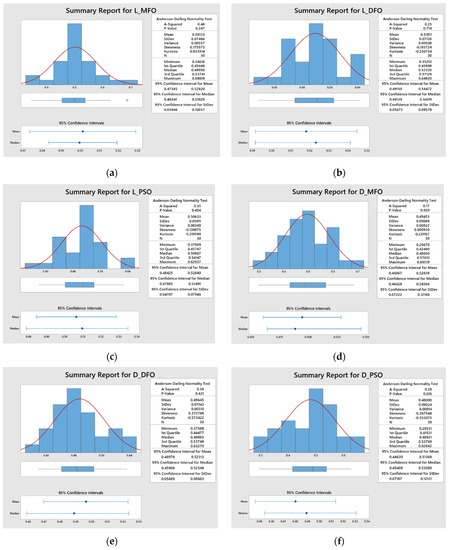
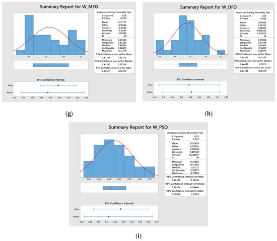
Figure 4. Statistical analysis of closeness values for (a) Response L-MFO; (b) Response L-DFO; (c) Response L-PSO; (d) Response D-MFO; (e) Response D-DFO; (f) Response D-PSO; (g) Response W-MFO; (h) Response W-DFO; (i) Response W-PSO.

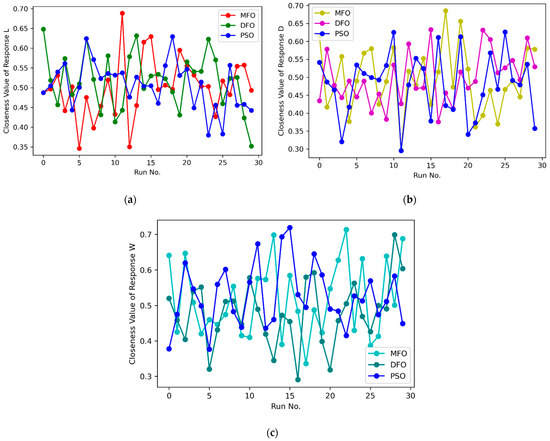
Figure 5. Comparison of closeness values for (a) Response L; (b) Response D; (c) Response W.

Figure 4a–c. represent the statistical distribution of closeness values obtained for 30 runs from Minitab 19 software using MFO, DFO and PSO algorithms for response L. Similar representation for responses D and W are illustrated in Figure 4d–f. and Figure 4g–i. respectively. It is observed that all of the p-values are greater than 0.05, which shows that the closeness values are normally distributed. This confirmed that the results obtained by the MFO, DFO, and PSO algorithms are accepted. Figure 5a–c. illustrate the closeness values obtained for various responses using MFO, DFO, and PSO algorithms for responses L, D and W respectively. It is understood that, in most of the runs, the MFO has the highest closeness value as compared to the DFO and PSO algorithms. Based on the highest closeness value, the best SVR model has been selected for each response, L, D, and W, and presented in Table 9. Using these models, the predicted response values are calculated and represented in Figure 6. The actual training data set of responses, L, D, and W, with their predicted values are plotted in Figure 6a–c. A similar representation is shown for the testing data set in Figure 6d–f. The predicted values of L and W are closer to the actual value in the training data set compared with response D. In the testing data set, out of 29 samples of response W, almost all predicted values are closer to the actual values, whereas in L, out of 20 samples, 14 are closer, and in D, it is only 7 out of 25. It is inferred that the SVR models developed to predict the response values of L and W are more accurate compared to D. The probability plots shown in Figure 7a–c. reveal that the results obtained using MFO for 30 runs are normally distributed for trainnig data set of responses L, D and W. Figure 7d–f. represent probability plots for testing data set of responses L, D and W, it also show the results are normally distributed; hence, the developed SVR models are appropriate. The three performance measures of SVR models for responses, L, D, and W, are presented in Figure 8a–c. It is reported that RMSE values of 0.071, 0.0767, and 0.0678 were obtained in the testing data set of responses L, D, and W, respectively. Lesser MAE values of 0.0624, 0.0672, and 0.0583 and higher $R^2$ values of 0.9996, 0.9909, and 0.9999 were reported in the testing data set. Figure 9 illustrates the convergence plot of performance measures for three responses, L, D, and W, for the total, training, and testing data sets. It is observed from Figure 9a–c that the convergence occurred on the 34th, 41st, and 34th iterations in the MFO algorithm, whereas, in DFO, it occurred on the 52nd, 52nd, and 55th iterations in response L. It is confirmed from Figure 9d–f. that the convergence occurred on the 40th, 54th, and 48th iterations in the MFO algorithm, whereas, in DFO, it occurred on the 61st, 43rd, and 63rd iterations in response D. It is evident from Figure 9g–i. that the convergence occurred on the 40th, 41st and 45th iterations in the MFO algorithm, whereas, in DFO, it occurred on the 61st, 57th, and 67th iterations in response W. It is confirmed from Figure 9a–c. that the convergence occurred in PSO for response L will be at the 89th, 63rd and 87th iterations for RMSE, MAE, and R² values that are higher than the convergence iteration numbers in the MFO algorithm. It is also observed from Figure 9d–i. that the convergence occurred in a higher iteration number in the case of response D and W in the PSO algorithm compared with the MFO. Hence, the MFO algorithm outperformed compared to the DFO algorithm in the convergence of objective values.

Table 9. Best Parameters of the SVR model for responses L, D, and W.

Response	Kernel Function	Solver	Validation Scheme	Validation’s Scheme Parameter	% of Test Data	No. of Test Data
L	Linear	SMO	Holdout	14	17.1	20
D	Linear	SMO	Holdout	16	21.7	25
W	Linear	SMD	Holdout	15	25.2	29

Figure 6. Comparison of actual and predicted values for (a) Training Dataset-Response L; (b) Training Dataset-Response D; (c) Training Dataset-Response W; (d) Testing Dataset-Response L; (e) Testing Dataset-Response D; (f) Testing Dataset-Response W.

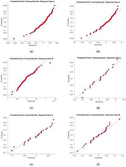
Figure 7. Probability Plot for (a) Training Dataset-Response L; (b) Training Dataset-Response D; (c) Training Dataset-Response W; (d) Testing Dataset-Response L; (e) Testing Dataset-Response D; (f) Testing Dataset-Response W.

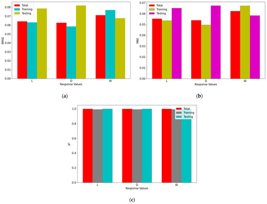
Figure 8. Performance measures of SVR models (a) RMSE; (b) MAE; (c) R².

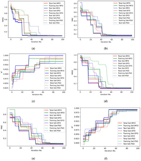
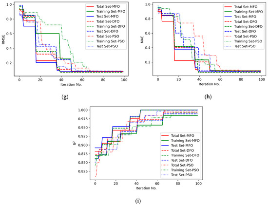
Figure 9. Convergence plot of performance of SVR for (a) Response L—RMSE; (b) Response L—MAE; (c) Response L—R²; (d) Response D—RMSE; (e) Response D—MAE; (f) Response D—R²; (g) Response W—RMSE; (h) Response W—MAE; (i) Response W—R².

Quantitative Comparison of MFO with DFO and PSO Algorithms

The performance of the MFO algorithm is compared with the DFO and PSO algorithms using two quantitative metrics, namely diversity and spacing [28]. Diversity indicates the spread of the Pareto solutions produced by an algorithm. The higher the value of diversity confirmed the better performance of the algorithm. The mathematical representation is given in Equation (18). Spacing is a straightforward method to compute the distance between the point and its closest neighbor. The minimum value of spacing indicates the better performance of the algorithm. The value of spacing is calculated using Equation (19). Table 10 represents the diversity and spacing values of the MFO, DFO, and PSO algorithms.

$$Div={\sum }_{i=1}^{np}{\left(P_{imax}-P_{imin}\right)}^2$$

(18)

where

P_imax—Maximum value of ith performance measures

P_imin—Minimum value of ith performance measures

np—number of performance measures

$$SP=\sqrt{\frac{1}{np-1}}{\sum }_{i=1}^{np}{\left(\overline{D}-D_i\right)}^2$$

(19)

where

$$\overline{D}=\frac{{\sum }_{i=1}^{np}{D}_i}{np}$$

$$D_i=\underset{i=1,2,\dots np}{\min }{\left\{\sum _{j=1}^{nr}abs\left(P_{ij}-P_{kj}\right)\right\}}_{k=i+1,\dots np}$$

where nr—Number of runs, I—index for a no. of performance measures, J—index for a no. of runs.

Table 10. Comparison of performance of algorithms using performance indicators.

Response	Algorithms	Diversity	Spacing
L	MFO	0.0652	0.0053
	DFO	0.0644	0.0054
	PSO	0.0648	0.0057
D	MFO	0.0679	0.0026
	DFO	0.0664	0.0058
	PSO	0.0653	0.0062
W	MFO	0.0685	0.0063
	DFO	0.0676	0.0066
	PSO	0.0680	0.0073

Table 10. Comparison of performance of algorithms using performance indicators.

Response	Algorithms	Diversity	Spacing
L	MFO	0.0652	0.0053
	DFO	0.0644	0.0054
	PSO	0.0648	0.0057
D	MFO	0.0679	0.0026
	DFO	0.0664	0.0058
	PSO	0.0653	0.0062
W	MFO	0.0685	0.0063
	DFO	0.0676	0.0066
	PSO	0.0680	0.0073

It is understood from Table 10 that the diversity value of the MFO algorithm is high compared to both the DFO and PSO algorithms in all of the three-response values, L, D, and W. Furthermore, the spacing value is less in the MFO algorithm for all three responses. Hence, it is confirmed that the MFO algorithm outperformed compared with both the DFO and PSO algorithms. The statistical analysis of three performance measures for training, testing, and total data sets for the MFO, DFO, and PSO algorithms are represented in Table 11, Table 12 and Table 13. The best values of three performance measures, RMSE, MAE, and $R^2$ are 0.0544, 0.0527, and 0.9999, respectively, for response L in the MFO algorithm, whereas in the DFO algorithm, the values are 0.0626, 0.0539, and 0.9993, and in the PSO algorithm, the values are 0.0626, 0.0538, and 0.9993. It is confirmed that the MFO algorithm is good compared to the DFO and PSO algorithms in predicting the response L. This is true for response W in the DFO algorithm, but in the PSO algorithm, both the RMSE and MAE values are lower compared with the MFO algorithm. In the case of response D in the DFO and PSO algorithms, the RMSE and MAE values are a little bit low compared to the MFO algorithm, but in the meantime, the $R^2$ value is higher than in the DFO and PSO algorithms. In overall performance, the SVR models developed by the MFO algorithm outperformed compared to the DFO and PSO algorithms.

Table 11. Statistical analysis of output obtained by the MFO algorithm.

Response	Statistics	MFO
		RMSE			MAE			${\mathit{R}}^2$
		Total	Training	Testing	Total	Training	Testing	Total	Training	Testing
L	Mean	0.0647	0.0628	0.0713	0.0556	0.0540	0.0631	0.9825	0.9807	0.9842
	StDev	0.0008	0.0008	0.0009	0.0009	0.0008	0.0008	0.0100	0.0108	0.0126
	Minimum	0.0631	0.0613	0.0697	0.0544	0.0527	0.0614	0.9631	0.9635	0.9606
	Q1	0.0641	0.0620	0.0706	0.0548	0.0534	0.0625	0.9744	0.9713	0.9708
	Median	0.0648	0.0627	0.0713	0.0556	0.0540	0.0631	0.9837	0.9785	0.9865
	Q3	0.0652	0.0633	0.0718	0.0565	0.0547	0.0638	0.9908	0.9906	0.9973
	Maximum	0.0660	0.0642	0.0730	0.0569	0.0554	0.0642	0.9998	0.9999	0.9996
	Range	0.0028	0.0029	0.0033	0.0025	0.0027	0.0029	0.0367	0.0365	0.0390
D	Mean	0.0804	0.0843	0.0697	0.0668	0.0693	0.0597	0.9767	0.9771	0.9810
	StDev	0.0011	0.0012	0.0009	0.0010	0.0010	0.0008	0.0121	0.0128	0.0125
	Minimum	0.0787	0.0821	0.0678	0.0653	0.0675	0.0583	0.9603	0.9600	0.9600
	Q1	0.0792	0.0834	0.0689	0.0659	0.0684	0.0590	0.9658	0.9667	0.9712
	Median	0.0804	0.0846	0.0699	0.0668	0.0695	0.0598	0.9743	0.9750	0.9809
	Q3	0.0813	0.0853	0.0704	0.0675	0.0701	0.0603	0.9844	0.9927	0.9945
	Maximum	0.0824	0.0861	0.0711	0.0683	0.0707	0.0611	0.9997	0.9970	0.9997
	Range	0.0037	0.0039	0.0033	0.0031	0.0032	0.0028	0.0394	0.0371	0.0398
W	Mean	0.0796	0.0830	0.0681	0.0657	0.0680	0.0586	0.9775	0.9804	0.9829
	StDev	0.0015	0.0012	0.0011	0.0011	0.0011	0.0011	0.0134	0.0120	0.0092
	Minimum	0.0771	0.0804	0.0665	0.0639	0.0663	0.0572	0.9604	0.9609	0.9609
	Q1	0.0784	0.0820	0.0669	0.0646	0.0669	0.0575	0.9670	0.9708	0.9769
	Median	0.0795	0.0831	0.0681	0.0657	0.0680	0.0581	0.9699	0.9812	0.9832
	Q3	0.0810	0.0840	0.0689	0.0668	0.0688	0.0596	0.9929	0.9903	0.9877
	Maximum	0.0818	0.0848	0.0702	0.0677	0.0701	0.0605	0.9999	0.9999	0.9999
	Range	0.0046	0.0044	0.0037	0.0039	0.0038	0.0033	0.0396	0.0390	0.0390

Table 12. Statistical analysis of output obtained by the DFO algorithm.

Response	Statistics	DFO
		RMSE			MAE			${\mathit{R}}^2$
		Total	Training	Testing	Total	Training	Testing	Total	Training	Testing
L	Mean	0.0656	0.0640	0.0729	0.0565	0.0549	0.0643	0.9806	0.9840	0.9850
	StDev	0.0010	0.0008	0.0009	0.0007	0.0008	0.0009	0.0125	0.0130	0.0101
	Minimum	0.0641	0.0626	0.0711	0.0554	0.0539	0.0625	0.9611	0.9613	0.9637
	Q1	0.0647	0.0633	0.0725	0.0558	0.0542	0.0635	0.9709	0.9734	0.9776
	Median	0.0657	0.0640	0.0728	0.0566	0.0545	0.0644	0.9787	0.9865	0.9878
	Q3	0.0666	0.0646	0.0738	0.0570	0.0555	0.0650	0.9931	0.9967	0.9930
	Maximum	0.0672	0.0655	0.0743	0.0580	0.0565	0.0654	0.9993	0.9993	0.9983
	Range	0.0031	0.0030	0.0033	0.0026	0.0026	0.0029	0.0382	0.0380	0.0347
D	Mean	0.0644	0.0598	0.0787	0.0549	0.0510	0.0690	0.9737	0.9714	0.9741
	StDev	0.0008	0.0008	0.0012	0.0007	0.0008	0.0010	0.0120	0.0112	0.0113
	Minimum	0.0630	0.0585	0.0767	0.0537	0.0497	0.0674	0.9531	0.9535	0.9518
	Q1	0.0637	0.0591	0.0778	0.0544	0.0503	0.0680	0.9629	0.9626	0.9664
	Median	0.0643	0.0599	0.0789	0.0548	0.0511	0.0693	0.9760	0.9699	0.9726
	Q3	0.0651	0.0606	0.0797	0.0554	0.0519	0.0700	0.9846	0.9797	0.9842
	Maximum	0.0658	0.0612	0.0803	0.0561	0.0522	0.0705	0.9906	0.9917	0.9905
	Range	0.0028	0.0027	0.0036	0.0024	0.0024	0.0032	0.0375	0.0382	0.0387
W	Mean	0.0804	0.0843	0.0697	0.0668	0.0693	0.0597	0.9767	0.9771	0.9810
	StDev	0.0011	0.0012	0.0009	0.0010	0.0010	0.0008	0.0121	0.0128	0.0125
	Minimum	0.0787	0.0821	0.0678	0.0653	0.0675	0.0583	0.9603	0.9600	0.9600
	Q1	0.0792	0.0834	0.0689	0.0659	0.0684	0.0590	0.9658	0.9667	0.9712
	Median	0.0804	0.0846	0.0699	0.0668	0.0695	0.0598	0.9743	0.9750	0.9809
	Q3	0.0813	0.0853	0.0704	0.0675	0.0701	0.0603	0.9844	0.9927	0.9945
	Maximum	0.0824	0.0861	0.0711	0.0683	0.0707	0.0611	0.9997	0.9970	0.9997
	Range	0.0037	0.0039	0.0033	0.0031	0.0032	0.0028	0.0394	0.0371	0.0398

Table 13. Statistical analysis of output obtained by the PSO algorithm.

Response	Statistics	PSO
		RMSE			MAE			${\mathit{R}}^2$
		Total	Training	Testing	Total	Training	Testing	Total	Training	Testing
L	Mean	0.0658	0.0640	0.0726	0.0567	0.0549	0.0639	0.9802	0.9800	0.9816
	StDev	0.0009	0.0009	0.0009	0.0008	0.0007	0.0009	0.0107	0.0104	0.0122
	Minimum	0.0642	0.0626	0.0710	0.0553	0.0538	0.0625	0.9600	0.9621	0.9609
	Q1	0.0654	0.0634	0.0721	0.0561	0.0542	0.0631	0.9721	0.9699	0.9727
	Median	0.0660	0.0639	0.0726	0.0568	0.0547	0.0640	0.9809	0.9810	0.9842
	Q3	0.0665	0.0647	0.0732	0.0573	0.0555	0.0646	0.9898	0.9883	0.9903
	Maximum	0.0672	0.0656	0.0743	0.0579	0.0562	0.0653	0.9980	0.9972	0.9993
	Range	0.0030	0.0031	0.0033	0.0026	0.0024	0.0029	0.0380	0.0351	0.0384
D	Mean	0.0660	0.0640	0.0729	0.0568	0.0552	0.0642	0.9818	0.9836	0.9779
	StDev	0.0009	0.0009	0.0010	0.0008	0.0008	0.0007	0.0118	0.0120	0.0109
	Minimum	0.0643	0.0627	0.0710	0.0554	0.0538	0.0628	0.9632	0.9612	0.9610
	Q1	0.0653	0.0633	0.0720	0.0563	0.0545	0.0637	0.9723	0.9769	0.9693
	Median	0.0663	0.0638	0.0729	0.0568	0.0553	0.0643	0.9802	0.9851	0.9775
	Q3	0.0668	0.0648	0.0737	0.0574	0.0560	0.0649	0.9931	0.9941	0.9846
	Maximum	0.0672	0.0654	0.0745	0.0580	0.0565	0.0655	0.9993	0.9996	0.9987
	Range	0.0030	0.0027	0.0035	0.0026	0.0027	0.0028	0.0361	0.0386	0.0377
W	Mean	0.0642	0.0626	0.0713	0.0554	0.0541	0.0626	0.9826	0.9793	0.9811
	StDev	0.0008	0.0008	0.0011	0.0008	0.0008	0.0010	0.0134	0.0111	0.0105
	Minimum	0.0629	0.0613	0.0696	0.0542	0.0528	0.0612	0.9612	0.9607	0.9603
	Q1	0.0635	0.0621	0.0703	0.0549	0.0534	0.0619	0.9698	0.9698	0.9773
	Median	0.0641	0.0626	0.0711	0.0553	0.0541	0.0624	0.9860	0.9808	0.9813
	Q3	0.0647	0.0630	0.0722	0.0560	0.0547	0.0636	0.9932	0.9871	0.9879
	Maximum	0.0656	0.0644	0.0730	0.0568	0.0554	0.0643	0.9998	0.9998	0.9996
	Range	0.0027	0.0030	0.0034	0.0026	0.0026	0.0030	0.0386	0.0393	0.0393

The comparison of the performance measures of the proposed method using MFO (PM-MFO) and the existing method using Feed Forward Back Propagation (EX-FFBP) by Daniel et al. [1] is illustrated in Figure 10. It is understood that, for the tested data set, the proposed method performed well for responses L in Figure 10a and for response W in Figure 10c as compared to response D in Figure 10b.

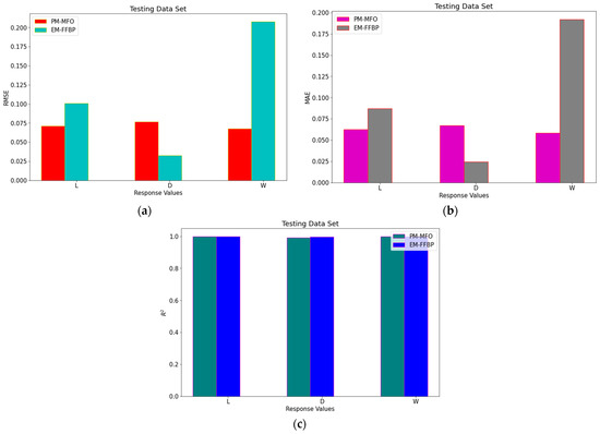
Figure 10. Comparison of performance measures (a) RMSE; (b) MAE (c) R².

4. Conclusions

In this work, SVR models have been developed to predict the length, depth, and width of the defect images using the given GLCM features extracted from MFL images. Five different parameters that decide the performance of SVR have been considered and three various performance measures, RMSE, MAE, and $R^2$ values, are taken into consideration to evaluate the performance of the SVR models. The MFO algorithm is implemented to find the best parameters of SVR models, and both DFO and PSO algorithms are used to compare the performance of the MFO algorithm. The normality test, probability, and residual plots have ensured that the results obtained using these algorithms are normally distributed and hence, accepted. The convergence, diversity, and spacing of performance measures are considered to evaluate the betterment of the functioning of the MFO with the DFO and PSO algorithms. Low convergence, a high value of diversity, and a low value of spacing reported at 34 iterations, 0.0685 and 0.0026, respectively, obtained with the MFO algorithm confirmed that it outperformed the DFO and PSO algorithms. The reported values of the three performance measures of SVR models, RMSE, MAE, and $R^2$ values of responses L, D, and W using the MFO algorithm, are 0.0527, 0.0613, and 0.9999. These lower values in both RMSE and MAE and high values in $R^2$ confirmed the performance of the MFO algorithm. Furthermore, in comparing the performance measures with the existing FFBP method, the proposed MFO–SVR method proved its effectiveness in responses L and W. The proposed SVR model is not suitable for a very large dataset, and all the features have been considered without finding the priority features. As a future work, this work can be extended further by adding the other additional features of GLSM extracted from the MFL image with data augmentation for different L, D, and W. Furthermore, features can be prioritized using the existing different algorithms, and based on that, the performance of the SVR models can be studied further.

References

- Daniel, J.; Abudhahir, A.; Paulin, J.J. Magnetic Flux Leakage (MFL) Based Defect Characterization of Steam Generator Tubes Using Artificial Neural Networks. J. Magn. 2017, 22, 34–42. [Google Scholar] [CrossRef]
- Raj, B.; Jayakumar, T.; Rao, B.P.C. Non-Destructive Testing and Evaluation for Structural Integrity. Sadhana 1995, 20, 5–38. [Google Scholar] [CrossRef]
- Dwivedi, S.K.; Vishwakarma, M.; Soni, A. Advances and Researches on Non Destructive Testing: A Review. Mater. Today Proc. 2018, 5, 3690–3698. [Google Scholar] [CrossRef]
- Göktepe, M. Non-Destructive Crack Detection by Capturing Local Flux Leakage Field. Sens. Actuators A Phys. 2001, 91, 70–72. [Google Scholar] [CrossRef]
- Ling, Z.W.; Cai, W.Y.; Li, S.H.; Li, C. A Practical Signal Progressing Method for Magnetic Flux Leakage Testing. Appl. Mech. Mater. 2014, 599–601, 782–785. [Google Scholar] [CrossRef]
- Wu, J.; Wu, W.; Li, E.; Kang, Y. Magnetic Flux Leakage Course of Inner Defects and Its Detectable Depth. Chin. J. Mech. Eng. 2021, 34, 63. [Google Scholar] [CrossRef]
- Ege, Y.; Coramik, M. A New Measurement System Using Magnetic Flux Leakage Method in Pipeline Inspection. Measurement 2018, 123, 163–174. [Google Scholar] [CrossRef]
- Shi, Y.; Zhang, C.; Li, R.; Cai, M.; Jia, G. Theory and Application of Magnetic Flux Leakage Pipeline Detection. Sensors 2015, 15, 31036–31055. [Google Scholar] [CrossRef]
- Suresh, V.; Abudhahir, A.; Daniel, J. Development of Magnetic Flux Leakage Measuring System for Detection of Defect in Small Diameter Steam Generator Tube. Measurement 2017, 95, 273–279. [Google Scholar] [CrossRef]
- Jin, C.; Kong, X.; Chang, J.; Cheng, H.; Liu, X. Internal Crack Detection of Castings: A Study Based on Relief Algorithm and Adaboost-SVM. Int. J. Adv. Manuf. Technol. 2020, 108, 3313–3322. [Google Scholar] [CrossRef]
- Zhang, J.; Teng, Y.-F.; Chen, W. Support Vector Regression with Modified Firefly Algorithm for Stock Price Forecasting. Appl. Intell. 2018, 49, 1658–1674. [Google Scholar] [CrossRef]
- Kari, T.; Gao, W.; Tuluhong, A.; Yaermaimaiti, Y.; Zhang, Z. Mixed Kernel Function Support Vector Regression with Genetic Algorithm for Forecasting Dissolved Gas Content in Power Transformers. Energies 2018, 11, 2437. [Google Scholar] [CrossRef]
- Houssein, E.H. Particle Swarm Optimization-Enhanced Twin Support Vector Regression for Wind Speed Forecasting. J. Intell. Syst. 2017, 28, 905–914. [Google Scholar] [CrossRef]
- Li, S.; Fang, H.; Liu, X. Parameter Optimization of Support Vector Regression Based on Sine Cosine Algorithm. Expert Syst. Appl. 2018, 91, 63–77. [Google Scholar] [CrossRef]
- Yuan, F.-C. Parameters Optimization Using Genetic Algorithms in Support Vector Regression for Sales Volume Forecasting. Appl. Math. 2012, 03, 1480–1486. [Google Scholar] [CrossRef]
- Papadimitriou, T.; Gogas, P.; Stathakis, E. Forecasting Energy Markets Using Support Vector Machines. Energy Econ. 2014, 44, 135–142. [Google Scholar] [CrossRef]
- Gayathri, R.; Rani, S.U.; Cepova, L.; Rajesh, M.; Kalita, K. A Comparative Analysis of Machine Learning Models in Prediction of Mortar Compressive Strength. Processes 2022, 10, 1387. [Google Scholar] [CrossRef]
- Gupta, K.K.; Kalita, K.; Ghadai, R.K.; Ramachandran, M.; Gao, X.Z. Machine Learning-Based Predictive Modelling of Biodiesel Production—A Comparative Perspective. Energies 2021, 14, 1122. [Google Scholar] [CrossRef]
- Ganesh, N.; Joshi, M.; Dutta, P.; Kalita, K. PSO-tuned Support Vector Machine Metamodels for Assessment of Turbulent Flows in Pipe Bends. Eng. Comput. 2019, 37, 981–1001. [Google Scholar] [CrossRef]
- Jayasudha, M.; Elangovan, M.; Mahdal, M.; Priyadarshini, J. Accurate Estimation of Tensile Strength of 3D Printed Parts Using Machine Learning Algorithms. Processes 2022, 10, 1158. [Google Scholar] [CrossRef]
- Priyadarshini, J.; Elangovan, M.; Mahdal, M.; Jayasudha, M. Machine-Learning-Assisted Prediction of Maximum Metal Recovery from Spent Zinc–Manganese Batteries. Processes 2022, 10, 1034. [Google Scholar] [CrossRef]
- Mirjalili, S. Moth-Flame Optimization Algorithm: A Novel Nature-Inspired Heuristic Paradigm. Knowl.-Based Syst. 2015, 89, 228–249. [Google Scholar] [CrossRef]
- Abdelazim, G.H.; Mohamed, A.; El Aziz, M.A. A comprehensive review of moth-flame optimisation: Variants, hybrids, and applications. J. Exp. Theor. Artif. Intell. 2020, 32, 705–725. [Google Scholar] [CrossRef]
- Karthick, M.; Anand, P.; Siva Kumar, M.; Meikandan, M. Exploration of MFOA in PAC Parameters on Machining Inconel 718. Mater. Manuf. Process. 2021, 37, 1433–1445. [Google Scholar] [CrossRef]
- Ananthakumar, K.; Rajamani, D.; Balasubramanian, E.; Paulo Davim, J. Measurement and Optimization of Multi-Response Characteristics in Plasma Arc Cutting of Monel 400TM Using RSM and TOPSIS. Measurement 2019, 135, 725–737. [Google Scholar] [CrossRef]
- Mirjalili, S. Dragonfly Algorithm: A New Meta-Heuristic Optimization Technique for Solving Single-Objective, Discrete, and Multi-Objective Problems. Neural Comput. Appl. 2015, 27, 1053–1073. [Google Scholar] [CrossRef]
- Kumar, M.S.; Rajamani, D.; Nasr, E.A.; Balasubramanian, E.; Mohamed, H.; Astarita, A. A Hybrid Approach of ANFIS—Artificial Bee Colony Algorithm for Intelligent Modeling and Optimization of Plasma Arc Cutting on Monel™ 400 Alloy. Materials 2021, 14, 6373. [Google Scholar] [CrossRef]
- Khalilpourazari, S.; Khalilpourazary, S. Optimization of Time, Cost and Surface Roughness in Grinding Process Using a Robust Multi-Objective Dragonfly Algorithm. Neural Comput. Appl. 2018, 32, 3987–3998. [Google Scholar] [CrossRef]
Publisher’s Note: MDPI stays neutral with regard to jurisdictional claims in published maps and institutional affiliations. |
© 2022 by the authors. Licensee MDPI, Basel, Switzerland. This article is an open access article distributed under the terms and conditions of the Creative Commons Attribution (CC BY) license (https://creativecommons.org/licenses/by/4.0/).