An Extreme Learning Machine for the Simulation of Different Hysteretic Behaviors

Abstract

Hysteresis is a non−unique phenomenon known as a multi−valued mapping in different fields of science and engineering. Accurate identification of the hysteretic systems is a crucial step in hysteresis compensation and control. This study proposes a novel approach for simulating hysteresis with various features that combines the extreme learning machine (ELM) and least−squares support vector machine (LS−SVM). First, the hysteresis is converted into a single−valued mapping by deteriorating stop operators, a combination of stop and play hysteresis operators. Then, the converted mapping is learned by a LS−SVM model. This approach facilitates the training steps and provides more accurate results in contrast to the previous experimental studies. The proposed model is evaluated for several hystereses with various properties. These properties include rate−independent or rate−dependent, congruent or non-congruent, and symmetric or asymmetric problems. The results indicate the efficiency of the newly developed technique in terms of accuracy, computational cost, and convergence rate.

1. Introduction

Hysteresis is a phenomenon that is observed in a variety of systems including ferromagnetic materials, mechanical, piezoelectric [1], and magnetostrictive actuators [2]. The behavior of the restoring force exhibits hysteretic behavior in dynamic response analyses of nonlinear structural systems [3]. The word hysteresis is derived from a prehistoric Greek word that meant backwardness. It was invented in around 1890 by Alfred Ewing [4] to classify the behavior of magnetic materials. Hysteresis, in general, is the dependence of a system’s situation on its past. This lagging in hysteretic systems relies on changing the internal system state or rate dependence. A hysteretic system’s output is influenced by both its past and present inputs. The conversion of the hysteretic into a one-to-one mapping and the training of the converted mapping play a key role in hysteresis simulation. In this regard, multiple mathematical models have been proposed to characterize hysteresis in recent decades. Among these methods, Preisach model [5], Prandtl−Ishlinskii model, Krasnosel’skii−Pokrovskii model, Bouc−Wen model [6,7], Masing model [8] and Bouc−Wen−Baber−Noori (BWBN) model [9,10], have been widely used in the literature for hysteresis. Each of the abovementioned models is capable of simulating hysteresis with certain behavior. For instance, the Masing model can only simulate hysteresis, which is symmetric and rate-independent. The Preisach model can be operated for symmetric and asymmetric congruent hysteresis, the Prandtl model can be used for symmetric and rate-independent hysteresis, and the BWBN model can simulate strength, stiffness, and shear pinching behavior as well as asymmetry. Based on the mentioned models, many research studies have been performed. Mathematical models use some free parameters for the simulation of the hysteretic behaviors tuned through the identification process. Unfortunately, no unique mathematical form can be fully adopted for different cases. Artificial intelligence systems such as neural networks have found a special place [11,12]. Multilayer feed−forward neural networks (MFFNNs) as general approximation tools [13] are utilized in the identification of hysteretic behavior as model-free systems [14,15]. One of the MFFNNs’ drawbacks is that they are static systems with no internal memory. Nonlinear autoregressive exogenous (NARX) neural networks [16] rectify this lack by putting a past state memory in the input layer of the MFFNNs. Serpico and Visone [17] have utilized an MFFNN as part of the Preisach model to evaluate the mapping. In other research studies, Farrokh and Dizagi [18] utilized an MFFNN to simulate the hysteresis converted into a single-valued static mapping by Madelung’s rules.

Recently inspired by the Preisach and Prandtl models, new Artificial Neural Networks (ANNs) have been proposed [19,20,21,22]. They use stop and play operators in their activation functions. These activation functions make them successful in hysteresis simulation. However, they have some major drawbacks in practical implementation. In the neural network method, this is important to determine the neural network’s architecture before training. Unfortunately, there is no common way to assign the ANN architecture in terms of the number of hidden layers and the number of hidden neurons in every layer. Additionally, ANN creates overfitting problems by reaching a local minimum during training [23]. Overfitting is not a serious issue in Support Vector Machines (SVMs) compared to neural networks.

Furthermore, as a version of the SVM, the least-squares support vector machine (LS−SVM) uses equality equations rather than inequality constraints. LS−SVM is less complicated than SVM and more efficient computationally [24]. Another benefit of LS−SVM is that there are less parameters that need to be adjusted in order to detect hysteretic behaviors [25]. How to transfer a multiple-valued hysteretic behavior to a single-valued mapping is the most difficult problem in hysteretic simulation using the LS−SVM model. The literature contains several solutions that have been suggested. For example, piezoelectric actuator hysteresis has been transformed into a single-valued mapping by the LS−SVM model by Xu [26] using a NARX−based memory. Although his simulation was effective, hysteresis without measurable states cannot be completely recalled by NARX systems. As a result of the required feedback, they are vulnerable to error accumulation. In another research study, Farrokh [23] proposed an intelligent hysteretic model that utilizes the LS−SVM. This model was influenced by the Preisach hysteresis model, which transformed a hysteretic system into a single-valued mapping using hysteresis operators. An LS−SVM then picks this up and learns it. Compared to neural networks, the model has fewer over−fitting issues. Additionally, unlike neural−based models, this model is not concerned with identifying a suitable architecture. Due to the use of the LS−SVM component as an intelligent tool, it can actually be operated much more easily than the Preisach model. Additionally, because it is theoretically equivalent to the Preisach model, which is only appropriate for congruent hysteresis behavior, this model can produce congruent hysteresis loops.

This paper proposes an intelligent hysteresis model based on a combination of ELM and LS−SVM. The proposed model uses several deteriorating stop operators by which a hysteretic system is converted into a single−valued mapping. Then, the one−to−one mapping is learned by an LS−SVM. The paper structure is as follows. Firstly, short reviews of the deteriorating stop operator, LS−SVM, and ELM are undertaken. Then, the ELM−SVM architecture and its training algorithm are proposed. Finally, the capabilities of the proposed ELM−SVM model are assessed on several hysteretic systems with different behaviors. In this regard, the ELM−SVM model achievement compared with other models is investigated.

2. Deteriorating Stop Operator

A deteriorating stop (DS) operator is a composition of stop and play operators that have been proposed by Farrokh et al. [22]. Generally, two types of degradation can simultaneously occur in the hysteresis loops: degradation of stiffness and strength. These types of degradation occurred during the DS operator’s body slip [22]. Cumulative body slip is considered an indicator to evaluate the extent of damage. The computation in a DS operator has been summarized in Figure 1.

The symbols ${\epsilon }_r[.]$ and $P_r[.]$ denote, respectively, stop and play operators that have been defined in Ref. [22]. The cumulative body slip can be calculated according to the play operator by induction as:

$$S_r\left(t_{i+1}\right)=\left|P_r\left[x\left(t_{i+1}\right)\right]-P_r\left[x\left(t_i\right)\right]\right|+S_r\left(t_i\right),$$

(1)

where $S_r\left(t_i\right)$ is the cumulative slip at time $t_i$ with initial condition $S_r\left(t_0\right)=0$, $x\left(t_i\right)$= displacement. The DS operator output is gained with a soundness indicator in terms of the accumulative body slip. The following equation for the DS operator takes into account the soundness index’s most basic function:

$$B{L}_{r\beta }\left(S_r\right)=\{\begin{array}{c}1-\frac{S_r}{r\beta } |S_r<r\beta \\ 0 |S_r\ge r\beta \end{array},$$

(2)

where $r$ is friction force and $\beta$ is an index that controls the deterioration rate of the DS operator. The deterioration process in the DS operators is sped up by a small value of $\beta$. Thus, the DS operator’s mathematical, $D{S}_{r\beta }$, can be represented as:

$$D{S}_{r\beta }\left[x\left(t\right)\right]={ℇ}_r\left[x\left(t\right)\right]\times B{L}_{r\beta }\left(S_r\right),$$

(3)

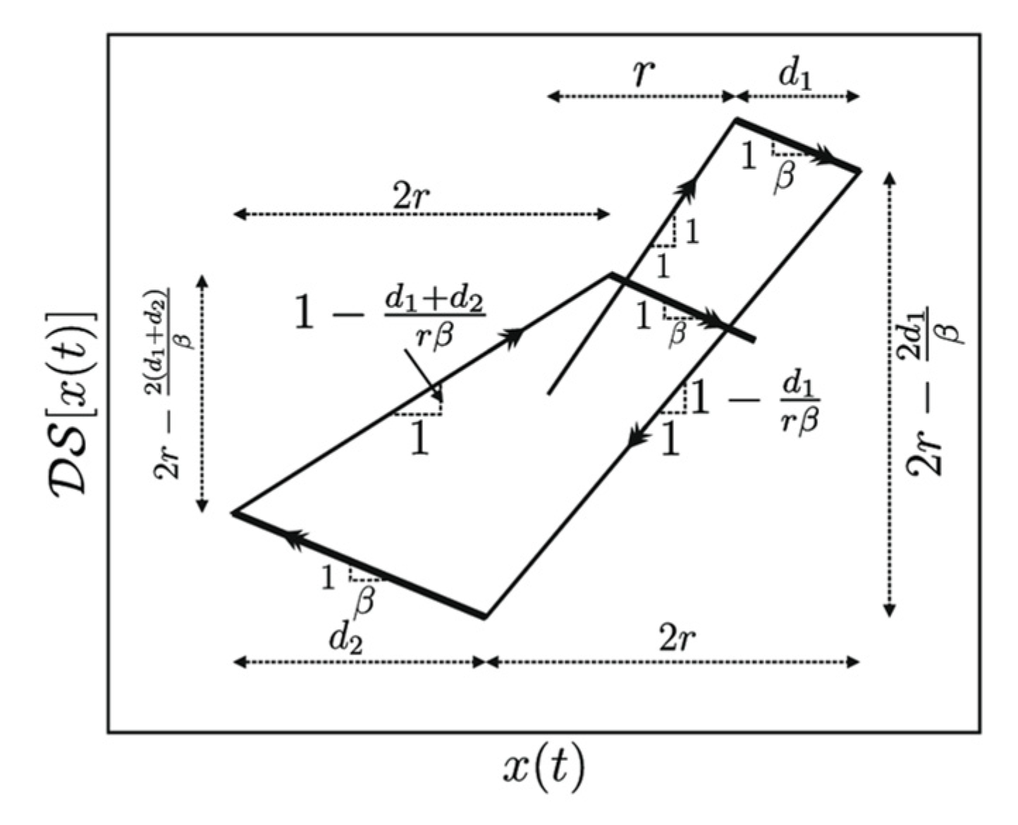
where ${ℇ}_r\left[x\left(t\right)\right]$ represents operator stop. The impacts of $r$ and $\beta$ on a DS operator hysteresis loop are shown in Figure 2. The rate of stiffness loss and strength deterioration are both governed by the $\beta$−value. Figure 2 shows that decreasing the $\beta$−value decreases both stiffness and strength.

The large value $\beta$ conduces to diminishing the degradation rate and transmutes a DS operator to a conventional stop operator.

3. Extreme Learning Machine

Extreme learning machines are special neural networks with a single hidden layer that are used for classification, regression, feature learning, and compression. The name of extreme learning machine (ELM) was given to such models by its main creator Guang-Bin Huang [27]. One of the salient features of ELM is that the connection between input and the first hidden layer neurons are randomly assigned and fixed during the training process. ELM can provide good generalization capacity with a faster learning speed, which can prevent much human interference [28]. The free parameters of the output layer are calculated by a least-squares method. Hence, the calculational cost is much less than any other neural networks [29].

4. Least−Squares Support Vector Machine

The least squares support vector machine is a development of the support vector machine that was suggested by Suykens and Vandewalle [24]. Instead of the inequality constraint in SVM, some equality constraints are used in LS−SVM. Hence, it obtains the final solution by dissolving a set of linear equations. This method has many advantages over the SVM method, which can increase computational efficiency, reduce complexity, and reduce training parameters. The following is a short overview of the LS−SVM’s concepts.

The LS−SVM uses a nonlinear function to transfer the input data $z$ into a high−dimensional feature space, where it subsequently uses a linear regressor to generate the predicted $\widehat{y}$. The regressor is described as:

$$\widehat{y}\left(z\right)=w^T\mathsf{\varphi }\left(z\right)+b$$

(4)

in which $w$ is the weights, $b$ is a scaler bias, and $\mathsf{\varphi }(·)$ represents an unknown nonlinear function. With the given the training dataset ${\left(z^k,y^k\right)}_{K=1}^N$, in which $N$ is the number of the training samples, its training can be conducted through an optimization problem in the primal weight space:

$$\min J_p\left(w,\mathit{e}\right)=\frac{1}{2}{w}^{T}w+\gamma \frac{1}{2}{\displaystyle \sum }_{k=1}^N{e}_k^2$$

(5)

where

$$y^k={\mathbf{w}}^T\mathsf{\varphi }\left({\mathbf{z}}^k\right)+b+e_k$$

(6)

Using the Lagrangian function

$$L\left(w,b,\mathit{e};\mathsf{\alpha }\right)=J_p\left(w,\mathit{e}\right)-{\displaystyle \sum }_{k=1}^N{\alpha }_k\left(w^T\mathsf{\varphi }\left(z^k\right)+b+e_k-y_k\right)$$

(7)

where ${\alpha }_k$ are Lagrange multipliers. The Karush–Kuhn–Tucker conditions can be used to transform the optimization problem from primal form to its dual form. The following linear set of equations can be used to obtain the parameters $\alpha$ and $b$ under these conditions and by omitting out the variables $w$ and $\mathit{e}$:

$$\left[\begin{array}{cc}0& 1_N^T\\ 1_N& \Omega +\frac{I}{\gamma }\end{array}\right]\left[\begin{array}{c}b\\ \mathsf{\alpha }\end{array}\right]=\left[\begin{array}{c}0\\ \mathbf{y}\end{array}\right]$$

(8)

where $y={\left[y^1,\dots ,y^N\right]}^T$, $1_N={\left[1,\dots ,1\right]}^T$, $\mathsf{\alpha }={\left[{\alpha }_1, \dots , {\alpha }_N\right]}^T$ is called the support vector and $I$ is an identity matrix. In addition, $\gamma$ is the regularization parameter. This parameter makes a balance between the squared error terms and weight decay in Equation (5). Additionally, the kernel trick is adopted to obtain the Gram matrix as follows:

$${\Omega }_{kl}=\mathsf{\varphi }{\left(z^k\right)}^T\mathsf{\varphi }\left(z^l\right)=K\left(z^k,z^l\right), k, l=1, 2, \dots , N$$

(9)

where $K\left(·,·\right)$ represents a predetermined kernel function. The kernel’s purpose is to prevent the calculation of the mapping $\mathsf{\varphi }(·)$, explicitly. The LS−SVM prediction is as:

$$\widehat{y}\left(z\right)={\displaystyle \sum }_{k=1}^N{\alpha }_k K\left(z,z^k\right)+b$$

(10)

where ${\alpha }_k$ and $b$ are the linear set’s solution of Equation (8) and $K\left(·,·\right)$is the kernel that is satisfying Mercer’s condition. The radial base function (RBF) that can be used as a kernel function for nonlinear mapping is defined as

$$K\left(z,z^k\right)=\exp \left(-\frac{{\left|\left|Z-Z^k\right|\right|}^2}{{\sigma }^2}\right)$$

(11)

where $\Vert ·\Vert$ is Euclidean distance and $\sigma$ is the width parameter. With the devoted regularization parameter $\gamma$ and kernel parameter $\sigma$, the goal of the training is to specify the support values ${\alpha }_k$ and the bias $b$ by using Equation (8). The LS−SVM model’s great generalization capacity depends on the two hyperparameters, $\gamma$ and $\sigma$, being appropriately adjusted. The hyperparameter values in this paper are determined using the $k$−fold cross−validation technique.

5. ELM−SVM Model

In hysteresis modeling, hysteresis operators such as stop and play operators play a significant role. However, these operators and models based on these operators, particularly the Preisach and Prandtl models, are suitable only for congruent hysteresis. This paper uses DS operators that enjoy deterioration in their hysteresis loops to propose a new intelligent model for congruent and non−congruent hysteresis. This new model is a composite of ELM and LS−SVM concepts, and it is called the ELM−SVM model in this paper. The ELM−SVM model is an extension of the Generalized Prandtl Neural Network (GPNN) previously proposed by Farrokh et al. [22]. Compared to the GPNN model in which the hidden DS neurons are directly connected to the output layer, in the ELM−SVM model, between the hidden layer containing DS neurons and the output layer is where the LS−SVM is situated. There are two adjustable parameters for each DS neuron in the first hidden layer ($r_i$, ${\beta }_i$).

Noteworthy is the fact that $\beta -$values adjust the ELM−SVM model’s overall deterioration rate so that if all the ${\beta }_i$ have high values, the deteriorating capability will diminish. The training process of this model consists of two stages. By inspiring ELM concept, the free parameters of DS, which are $r_i$ and ${\beta }_i$ for $i=1, 2,\dots ,n$are randomly set, in the first step:

$$0<r_i<r_{max}$$

(12)

$$0<{\beta }_i<{\beta }_{max}$$

(13)

where $r_{max}$ and ${\beta }_{max}$ are the maximum values for $r_i$ and ${\beta }_i$, respectively, and $i=1, 2, \dots , n$ in which $n$ is the number of DS neurons. Preassigning internal parameters of DS neurons facilitates the learning process and reduces the computational cost the same as in ELMs. Additionally, the existence of an LS−SVM as an additional hidden layer in this model improves the capabilities of GPNN since the used LS−SVM in the second hidden layer is a nonlinear mapping. In the second step, an LS−SVM has been selected to train one−to−one mapping caused by DS operators. Compared to the neural networks, LS−SVMs enjoy error functions with an unrivaled global minimum according to their parameters $\mathsf{\alpha }$ and b. The LS−SVM would be trained by using Equation (8) with the preassigned hyperparameters $\sigma$ and $\gamma$. The LS−SVM’s high generalization capability depends on properly tuning these hyperparameters. The Nelder−Mead simplex algorithm [30] is used for tuning the hyperparameters. In other to prevent overfitting, the cross−validation approach has been adopted in this paper. It is an evaluation method that determines to what extent statistical analysis results on a dataset can be generalized and independent of the training data. $k$−fold cross−validation error has been considered an objective function of the tuning process. This approach divides the shuffled training dataset into $k$ smaller datasets or folds. The model is trained on $k-1$ folds each time, and then the resulting model is evaluated on the remaining part of the dataset using a performance measure. The training and evaluation steps are repeated $k$ times, and the average performance measure is reported as cross−validation performance.

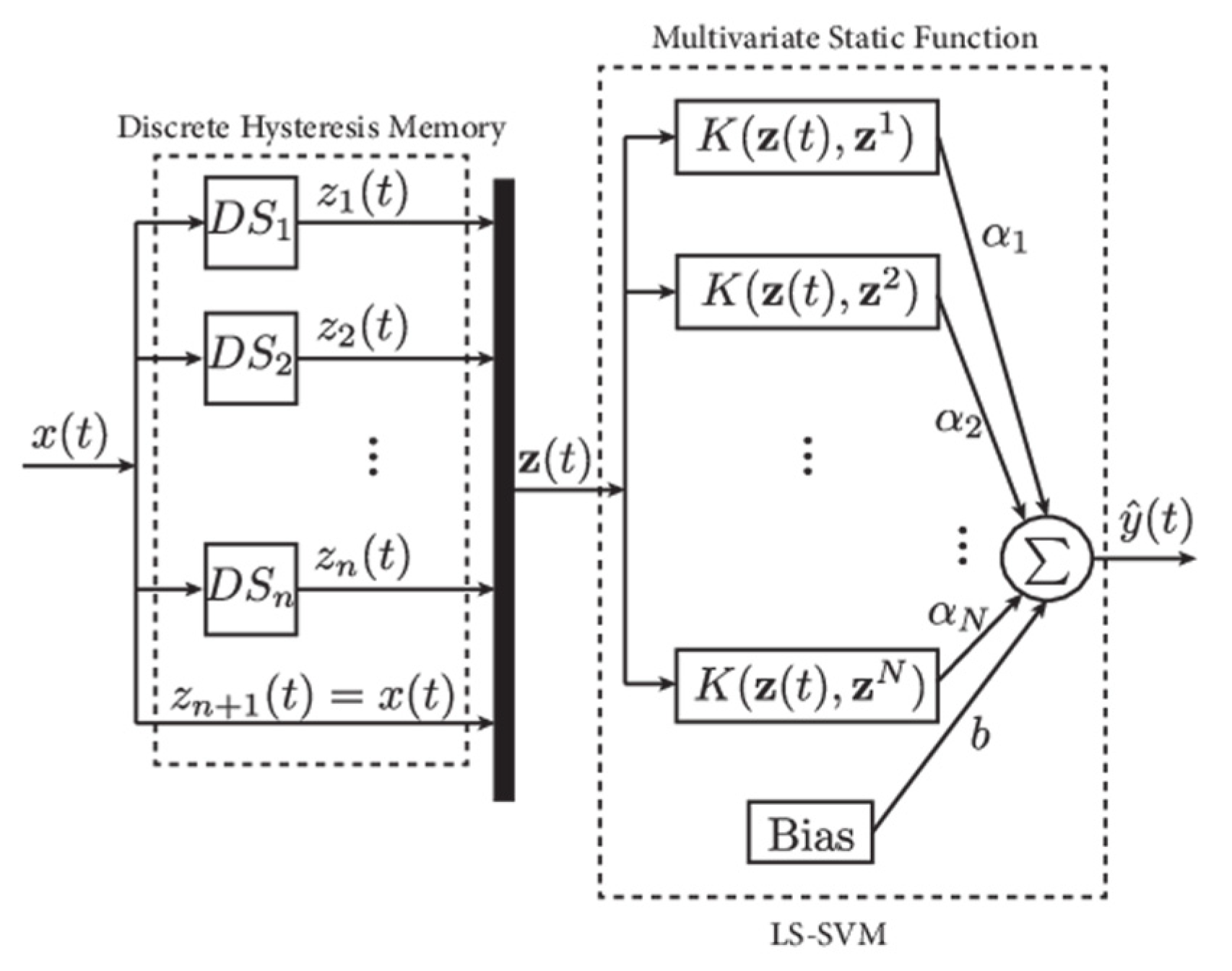
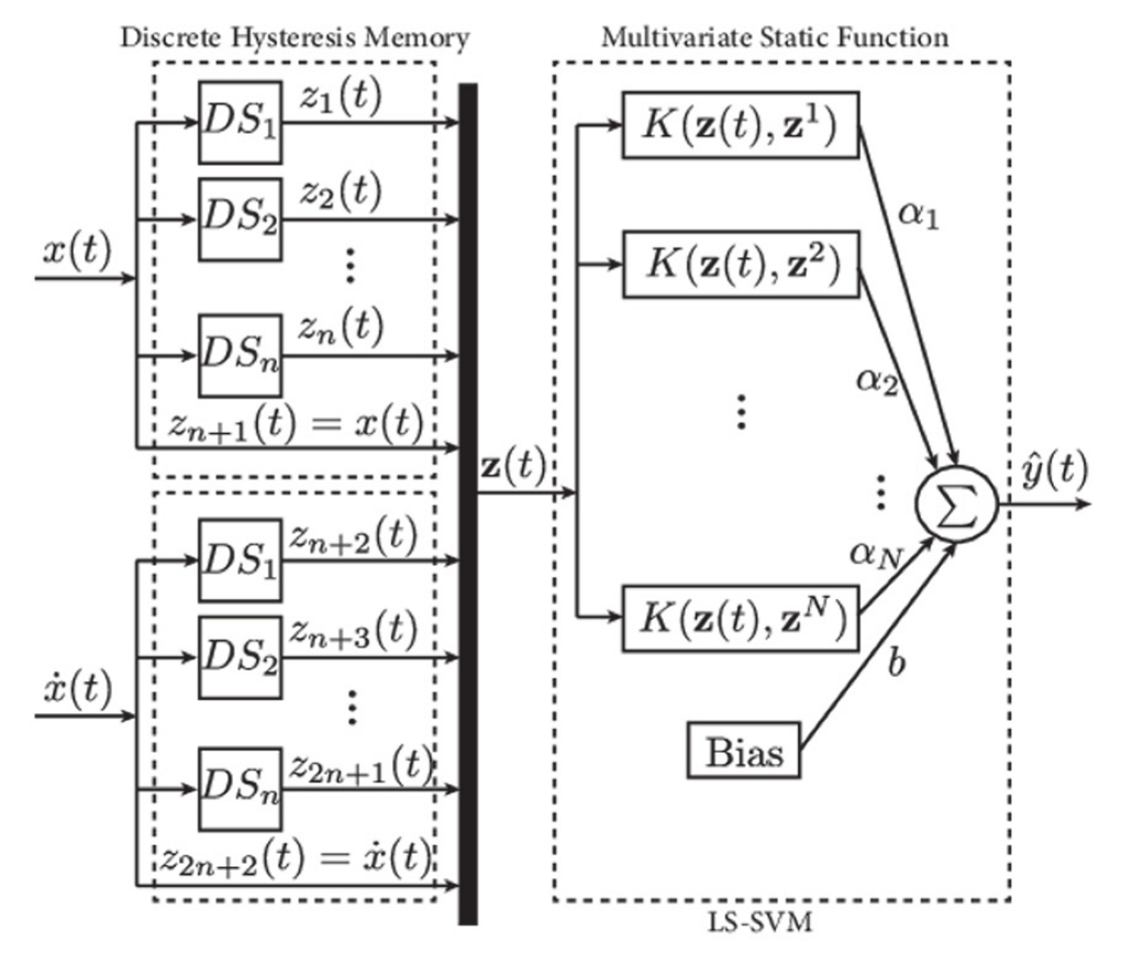
For the rate−dependent hystereses, an extra memory has been considered for the ELM−SVM model in this paper. It enhances the modeling accuracy of the presented model for rate−dependent hystereses. Details of the ELM−SVM model for both rate−independent and rate−dependent hystereses can be seen in Figure 3 and Figure 4, respectively.

The identification procedure of the ELM−SVM model is summarized as follows:

• Choose the appropriate number of DS neurons $n$ and the value of ${\beta }_{max}$;
• Set $r_{max}$ to ${\left|x\right|}_{max}$ and ${\dot{\left|x\right|}}_{max}$ for rate−independent and rate−dependent memories, respectively;
• Randomly set the internal DS neuron parameters $r_i$ and ${\beta }_{i }$considering Equations (12) and (13);
• The input vector of LS-SVM part of the model $z$ is calculated using the DS neurons as shown in Figure 3 or Figure 4;
• Using the Nelder−Mead method, the LS−SVM part’s hyperparameters are obtained based on the cross−validation approach. The internal parameters of LS−SVM, $\mathsf{\alpha }$ and $b$, are determined using Equation (8) during each iteration of the Nelder−Mead method.

6. Assessment of the ELM−SVM Model

In this section, a number of hystereses from diverse engineering domains have been examined in order to evaluate the capabilities of the ELM−SVM model. Experimental datasets have been adopted from several research studies in the field.

Although researchers applied different methods to identify these hysteretic behaviors, the proposed ELM−SVM model has been utilized in this paper. Additionally, in cases where they were available, the outcomes of other proposed models were compared with those of the ELM−SVM model.

6.1. Symmetric, Non−Congruent, and Rat−Independent Hysteresis

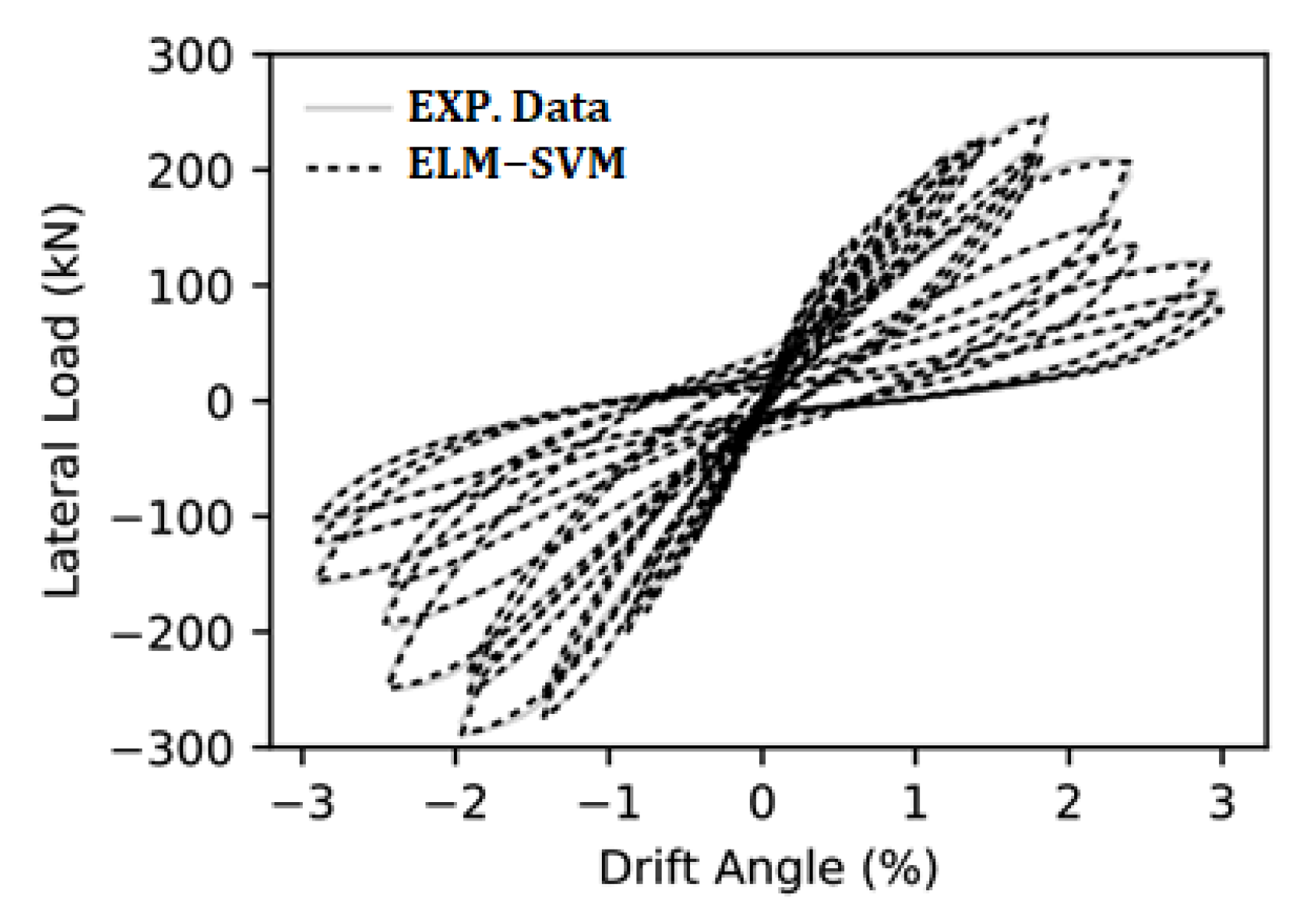
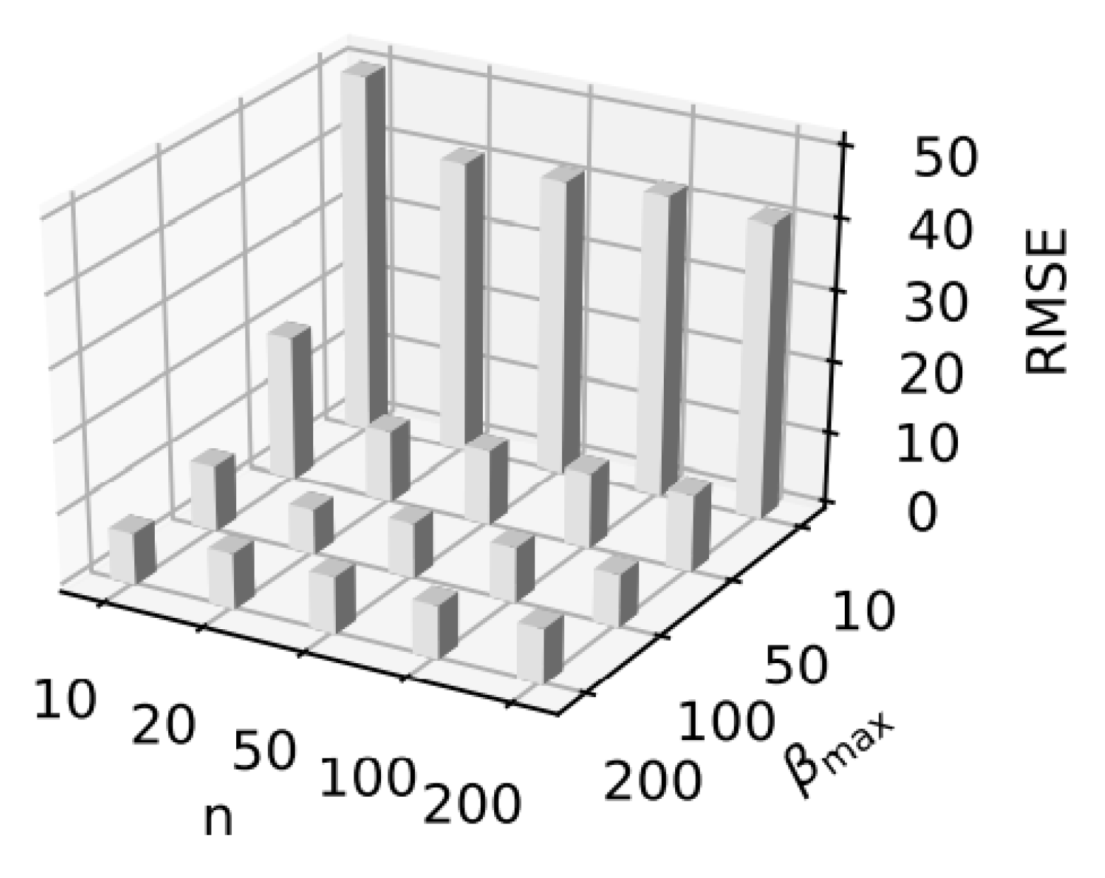
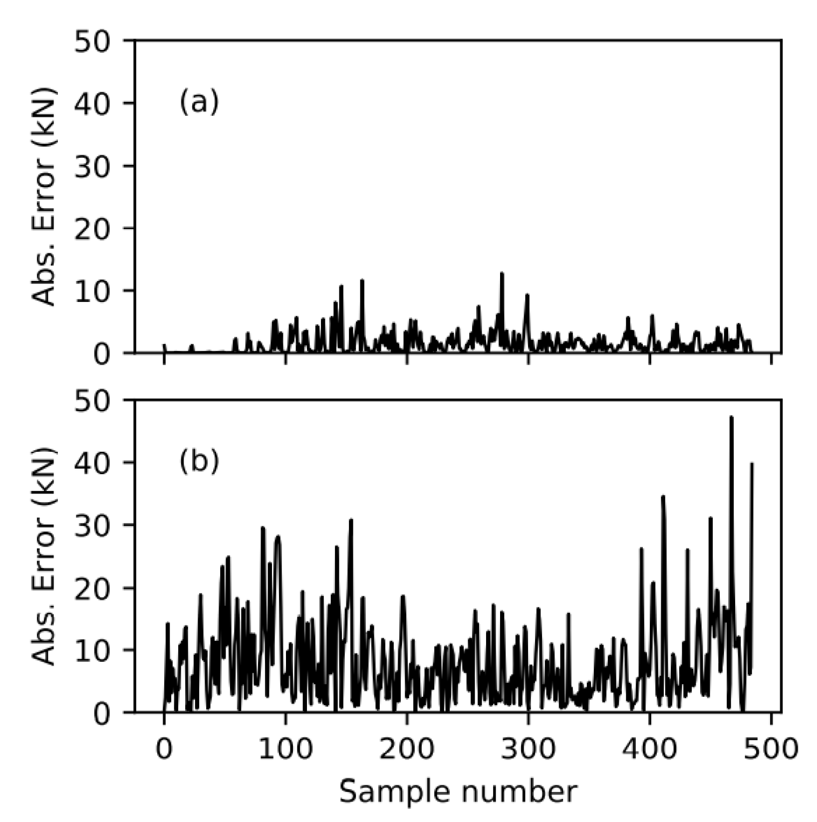
We make advantage of the findings from tests that Clyde et al. [31] carried out on an exterior beam−column joint of a multi−story concrete frame. They reported $x$ = drift ratio versus $y$ = the lateral load of the frame. As shown in Figure 5, the hysteretic behavior is non−congruent; thus, most Prandtl and Preisach−type models are not appropriate. Even if the hysteresis loops exhibit same extremum values as the damage index is increased, the loops become non−congruent. In addition, the hysteresis loops in this example are rate−independent and non−Masing. Since the PNN model can only learn congruent Masing hysteresis behaviors [22], they are not helpful in learning non-congruent hysteresis behaviors. The generalized Prandtl neural network (GPNN) was introduced by Farrokh et al. [22] to recognize deteriorating hysteretic behavior (GPNN). They also used their new proposal in this case. It is possible to train non−congruent and non−Masing hysteretic behavior using GPNN. However, it has no universal ability to precisely learn these behaviors because GPNN is a linear combination of different DS neurons. It lacks a nonlinear mapping between DS neurons in the hidden layer and output layer. Therefore, the ELM−SVM model is superior to GPNN as it uses LS−SVM for nonlinear mapping. The ELM−SVM model has been utilized to learn this hysteretic behavior. Figure 4 shows the architecture of the ELM−SVM model used in this example. As mentioned in the previous section, the number of the DS neurons $n$ and the value of ${\beta }_{max}$ should be appropriately chosen. For this purpose, the grid search method has been utilized, and its results have been depicted in Figure 6. Root mean square error (RMSE) has been considered as a performance measure for comparing different models. Figure 6 shows that the model with 20 DS neurons and ${\beta }_{max}$ = 100 outperforms the others. In Figure 5 hysteresis obtained from the ELM−SVM has been compared with experimental data, and it can be seen that there are in excellent agreement. For the purpose of showing the efficiency of the ELM−SVM model, the comparison between the ELM−SVM response and the other model is helpful. Figure 7a,b depict a comparison between the absolute error value of ELM−SVM model and GPNN model [22], respectively. It is obvious that ELM−SVM outperforms GPNN for this experimental data.

6.2. Asymmetric Non−Congruent Rate−Independent Hysteresis

In this illustration, we make use of the findings from tests conducted by Sinha et al. [32]. They investigated the cyclic uni−axial compression response of plain concrete. They investigated the stress−strain relationships for the cyclic loading-induced concrete hysteresis. They measured $x$ for strain and $y$ for stress in their studies. Given that the stress–strain relations for concrete under cyclic loading exhibit hysteresis behavior and are asymmetric, non−congruent, and non−Masing. Therefore, Preisach−type, PNN, and GPNN models cannot accurately learn this type of hysteresis behavior. For this case, the ELM−SVM model has also been taken into account. Figure 8 displays both the simulated and experimental hysteresis loops from the proposed model in this paper. Based on the available measured data, it was shown that the ELM−SVM is valid for predicting the asymmetric, non−Masing, and non−congruent hysteresis loops. This example has been trained with 5000 DS neurons, ${\beta }_{max}$ = 50 and 452 training data. Different values of $n$ and ${\beta }_{max}$ have been tried in this example to get the best result and the stated values (n = 5000 and ${\beta }_{max}$ = 50) are the optimized value. With these values, the training time is 15 s. It should be noted that the internal parameters of an LS−SVM do not depend on its input dimension. Hence, the increase in DS neuron number in ELM−SVM does not increase the risk of its overfitting. In LS−SVMs, the number of support vectors as adjustable parameters equals the number of cases in the training dataset. Thus, overfitting can be easily tackled in the ELM−SVM model by tuning the hyper−parameters $\gamma$ and σ. The learning curve of this example is shown in Figure 9. The training and cross−validation errors have more or less the same values in Figure 9 indicating that the trained ELM−SVM model has not overfitted the training data in this example.

6.3. Asymmetric Non−Masing Rate−Independent Hysteresis

Magnetostrictive property is the strong coupling phenomenon between some ferromagnetic materials’ magnetic and mechanical properties. Shape memory, magnetostrictive, and piezoelectric alloys are regarded as intelligent materials having in−built sensing and actuation capabilities. For this case, studies on a magnetostrictive actuator have been carried out by Tan and Baras [33,34]. When the input current of the actuator operated in a low−frequency region (typically below 5 Hz), the actuator’s response was remarkably rate-independent. In this phase, they have looked into the properties of the major and minor hysteresis loops [34]. The tested magnetostrictive actuator was subjected to rising triangular input currents with amplitudes between −0.7 and 1.2 A.

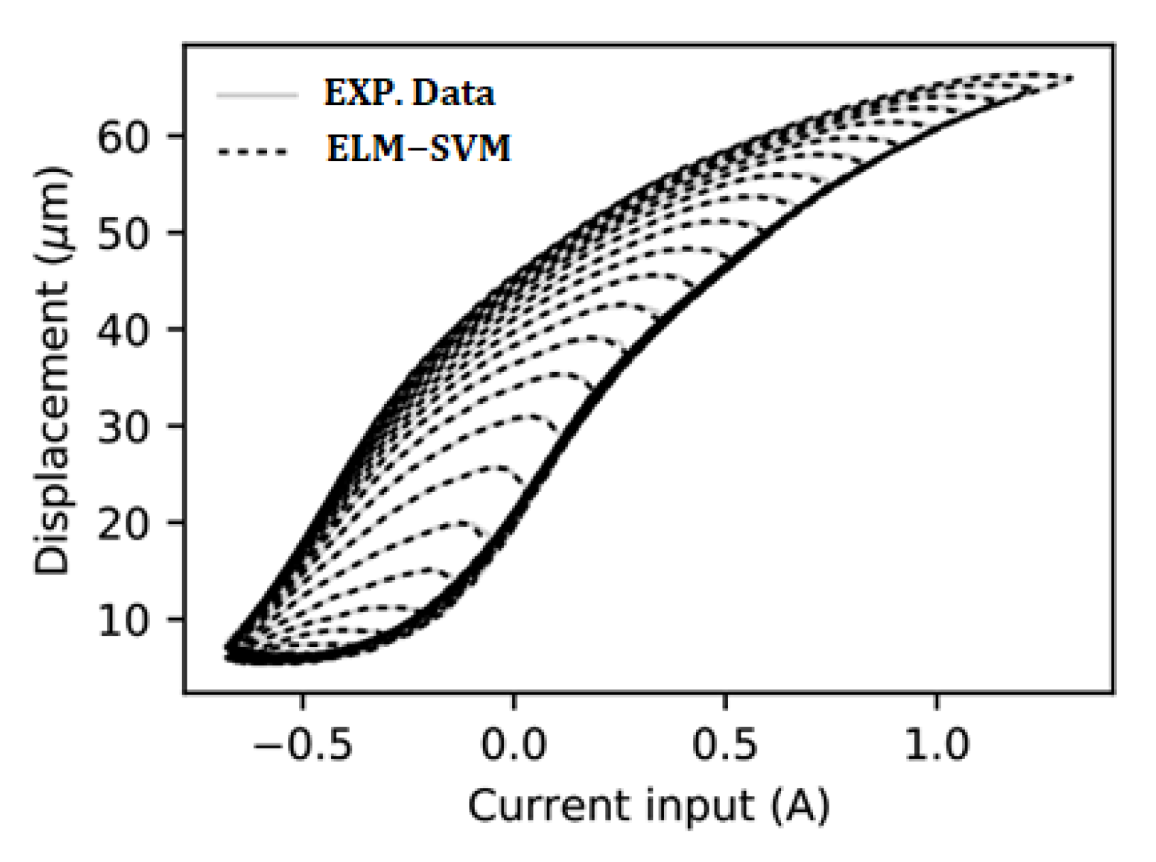
In Figure 10 solid gray curves represent the measured output displacement vs. input current relationships for the magnetostrictive actuator. This dataset has been used to evaluate the proposed model. The same as the previous example, an ELM−SVM model with $n=5000$ and ${\beta }_{max}=$50 has been considered for this hysteretic behavior. As in the previous example, these values are optimized values. The magnetostrictive actuator’s ELM−SVM response is contrasted with the measured data in Figure 10. The findings suggest that the ELM−SVM can accurately anticipate the magnetostrictive actuator’s asymmetric non-Masing hysteresis features. In order to verify the priority of the proposed model with other models, a comparison between the absolute error of the ELM−SVM and the Generalized Prandtl−Ishlinskii Model (GPIM) proposed by Al Janaideh et al. [35] has been conducted in Figure 11. It shows that the model presented in this paper is more accurate than GPIM.

6.4. Symmetric Rate−Dependent Hysteresis

Piezoelectric translator (PZT) actuators are frequently employed due to their high output force speed and accuracy, large bandwidth, and quick response time [36,37,38]. However, the PZT actuators’ hysteresis is a rate−dependent phenomenon that greatly depends on the amplitudes and frequencies of the control input. Therefore, high−speed input applications cannot be used with the Preisach and Prandtl−Ishlinskii models. Gu and Zhu [38] conducted a number of tests using designed sinusoidal excitations at various frequencies between 1 and 300 Hz to illustrate the effects of hysteresis. The provided results for the piezoelectric actuator reveals approximately rate−dependent symmetric major and minor hysteresis loops under varying excitation of different magnitudes and frequencies [18]. In this paper, the aforementioned experimental data is used to validate the rate−dependence capabilities of ELM−SVM. For this purpose, $\dot{x}$ has been considered in the input layer of the ELM−SVM as shown in Figure 4. Figure 12 shows the measured output displacement of the actuator versus input voltage for some frequencies by the proposed model as solid curves. A frequency has been tested to show the high performance of the ELM−SVM model. In Figure 12, all frequency responses contributed to training. However, in Figure 13, all frequency responses except the 10 Hz frequency contributed to training, and the 10 Hz frequency response was tested. The outcomes demonstrate the ELM−SVM’s learning capacity, both for training and test data. It should be noted that, in this example, $n$ and β_max have identical values of 2.

6.5. Asymmetric Rate-Dependent Non-Congruent Hysteresis

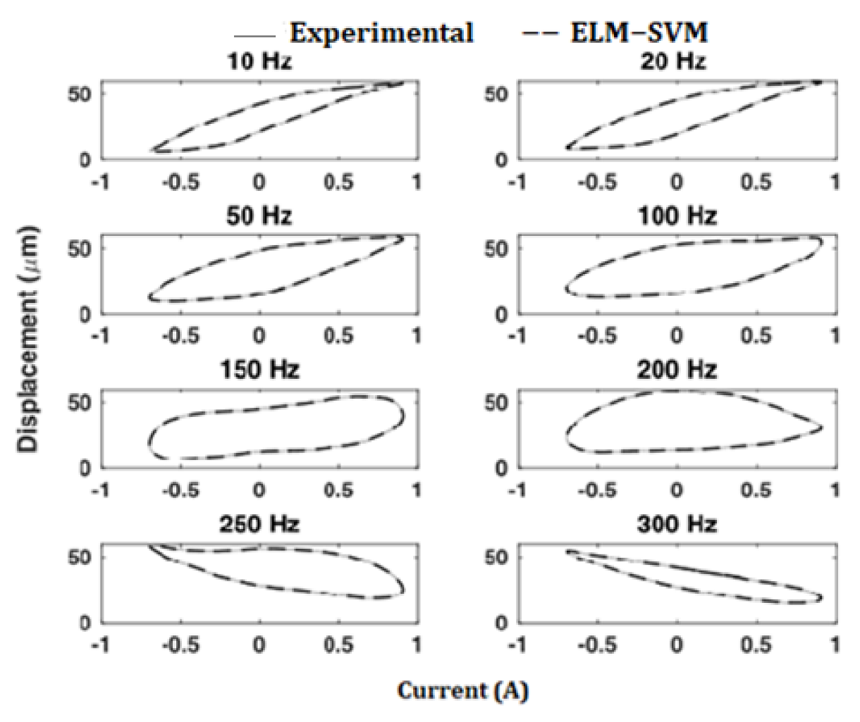
Magnetostrictive actuators are being used more frequently for vibration control and micro−positioning. In order to determine the magnetostrictive actuator’s hysteresis responses to sinusoidal input currents of constant amplitude (0.8 A) with a bias of 0.1 A over the frequency range of 10 to 300 Hz, Tan and Baras [33] performed laboratory testing. The results of this experiment demonstrate that the magnetostrictive actuator’s hysteresis loops between the input current and the output displacement are rate−dependent, non-congruent, and asymmetric, particularly for excitations above 10 Hz. The hysteresis characteristics of the magnetostrictive actuator at various stimulation frequencies are shown in Figure 14 as solid curves. The outputs under eight input frequencies, which vary from 10 to 300 HZ, show significant variances in the hysteresis loops. Magnetostrictive actuators have asymmetric, non-congruent, and extremely rate−dependent hysteresis loops. PNN, GPNN, and Preisach−type are hence unable to learn their behaviors. We used ELM−SVM to learn the rate-dependent behavior of magnetostrictive. The ELM−SVM model cannot only learn asymmetric and non-congruent hysteresis behavior, but it can also learn hysteresis loops with rate−dependency. Figure 14 shows dashed gray curves that are difficult to distinguish from solid gray curves to represent the hysteresis loops that the ELM−SVM model simulates (experimental data). For this case as well, it displays extremely low simulation errors. The ELM−SVM test has not been run in this instance because there is insufficient experimental data. Additionally, this example with $n=2$ and β_max = 2 has been trained on the prepared training dataset.

6.6. Hysteretic of Rate−Dependent

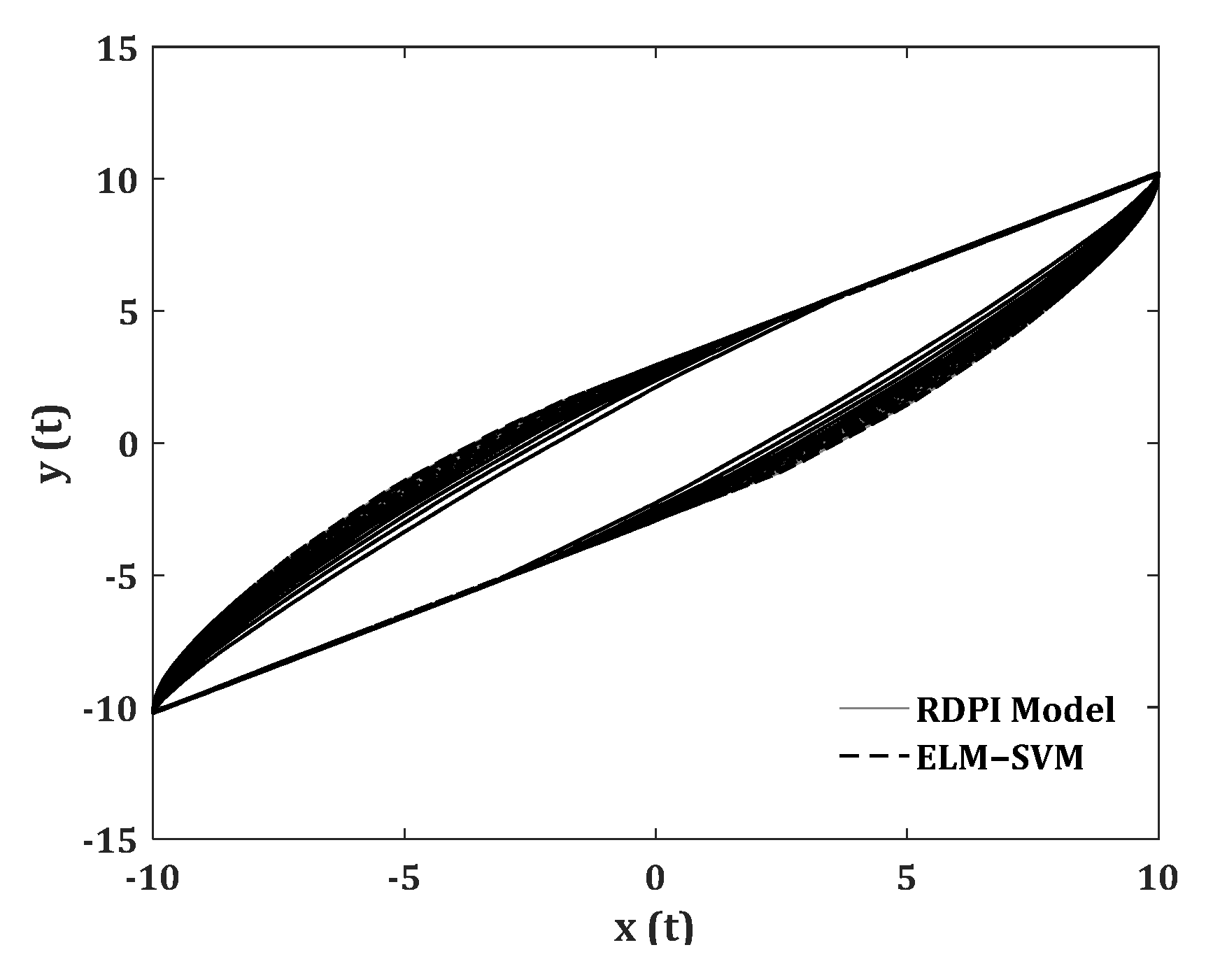
Recently, a rate−dependent Prandtl−Ishilinskii (RDPI) model was created in order to detect and manage rate−dependent hysteresis [39]. This model includes several play operators with various rate−dependent threshold values. More detailed information about the RDPI model can be discovered in [39]. In order to evaluate the proposed ELM−SVM hysteresis model, an RDPI model that generates rate-dependent hysteresis has been considered in this section. The hysteresis loops of the RDPI model under harmonic input signals with sweeping frequency are depicted in Figure 15. The input signal’s frequency affects the RDPI model’s output to some extent. The considered RDPI model was excited by a harmonic signal with a linear sweeping frequency from 10 to 40 Hz in order to produce the training samples for the ELM−SVM model. On the prepared training dataset and test, a rate-dependent ELM−SVM hysteresis model with $n=20$ and ${\beta }_{max}=2$ has been trained. It is worth mentioning that the test data has been attained for four distinct constant frequencies, 10 to 40 Hz, albeit the training data has had a continuous changeable frequency. Figure 16 shows the comparison of ELM−SVM responses and prepared test data. As can be seen, the errors in the test mode are negligible. The RMSE error values for the 10, 20, 30, and 40 Hz frequencies are 0.0930, 0.0157, 0.0247, and 0.0750, respectively. It indicates that the accuracy of the proposed model for this example is very high.

7. Conclusions

Based on the ELM and LS−SVM learning capabilities, the model for different hysteretic behaviors is proposed in this study as a novel approach. The suggested model employs a set of Deteriorating Stop neurons based on a special composition of the stop and play operators to first transform hysteresis, a multi−valued mapping, into a single−valued mapping. Free parameters for these DS neurons are chosen at random thanks to inspiration from an ELM.

Second, an LS−SVM is used to learn the mapping. The proposed hysteresis model is simpler to tune the adjustable parameters than the other Presiach−based model. Additionally, the Presiach model does not account for rate-dependent and non−congruent hysteresis. The use of the ELM−SVM model was discussed in light of the varied hysteresis features. Several hystereses from various disciplines were used to assess the proposed model.

The outcomes demonstrate that the ELM−SVM model performs excellently even for experimental data. The ELM−SVM hysteresis model demonstrated low generalization errors when its generalizability was tested. Furthermore, the results show that overfitting in the ELM−SVM model does not have significant effects because the training data size affects the model’s trainable parameter number. Finding the ideal architecture for the ELM−SVM model is less important than for neural−based models. This study used a fixed-architecture ELM−SVM to learn high-precision different adopted hystereses for training and test data.

The proposed ELM−SVM model has been assessed on different hysteretic behaviors from different fields of engineering in this paper. However, further assessments and application of this proposed model on hysteresis control and compensation remain open for future research.

References

1. Chen, Y.; Qiu, J.; Palacios, J.; Smith, E.C. Tracking control of piezoelectric stack actuator using modified Prandtl–Ishlinskii model. J. Intell. Mater. Syst. Struct. 2012, 24, 753–760. [Google Scholar] [CrossRef]
2. Liu, X.; Wu, Y.; Zhang, Y.; Wang, B.; Peng, H. Inverse model–based iterative learning control on hysteresis in giant magnetostrictive actuator. J. Intell. Mater. Syst. Struct. 2013, 25, 1233–1242. [Google Scholar] [CrossRef]
3. Baber, T.T.; Noori, M.N. Random vibration of degrading, pinching systems. J. Eng. Mech. 1985, 111, 1010–1026. [Google Scholar] [CrossRef]
4. Chatterjee, S. Parasuchus hislopi Lydekker, 1885 (Reptilia, Archosauria): Proposed replacement of the lectotype by a neotype. Bull. Zool. Nomencl. 2001, 58, 34–36. [Google Scholar]
5. Preisach, F. Über die magnetische Nachwirkung. Z. Für Phys. 1935, 94, 277–302. [Google Scholar] [CrossRef]
6. Wen, Y.-K. Method for random vibration of hysteretic systems. J. Eng. Mech. Div. 1976, 102, 249–263. [Google Scholar] [CrossRef]
7. Wen, Y. Methods of random vibration for inelastic structures. Appl. Mech. Rev. 1989, 42, 39–52. [Google Scholar] [CrossRef]
8. Masing, G. Eigenspannumyen und verfeshungung beim messing. Proc. Inter. Congr. Appl. Mech. 1926, 332–335. [Google Scholar]
9. Baber, T.T.; Noori, M.N. Modeling general hysteresis behavior and random vibration application. J. Vib. Acoust. 1986, 108, 411–420. [Google Scholar] [CrossRef]
10. Zhao, Y.; Noori, M.; Altabey, W.A.; Awad, T. A comparison of three different methods for the identification of hysterically degrading structures using BWBN model. Front. Built Environ. 2019, 4, 80. [Google Scholar] [CrossRef] [Green Version]
11. Noori, M.; Altabey, W.A. Hysteresis in Engineering Systems. Appl. Sci. 2022, 12, 9428. [Google Scholar] [CrossRef]
12. Wang, T.; Noori, M.; Altabey, W.A.; Farrokh, M.; Ghiasi, R. Parameter identification and dynamic response analysis of a modified Prandtl–Ishlinskii asymmetric hysteresis model via least-mean square algorithm and particle swarm optimization. Proc. Inst. Mech. Eng. Part L J. Mater. Des. Appl. 2021, 235, 2639–2653. [Google Scholar] [CrossRef]
13. Hornik, K. Approximation capabilities of multilayer feedforward networks. Neural Netw. 1991, 4, 251–257. [Google Scholar] [CrossRef]
14. Ghaboussi, J.; Garrett, J., Jr.; Wu, X. Knowledge-based modeling of material behavior with neural networks. J. Eng. Mech. 1991, 117, 132–153. [Google Scholar] [CrossRef]
15. Masri, S.F.; Chassiakos, A.G.; Caughey, T.K. Identification of nonlinear dynamic systems using neural networks. J. Appl. Mech. 1993, 60, 123–133. [Google Scholar] [CrossRef]
16. Siegelmann, H.T.; Horne, B.G.; Giles, C.L. Computational capabilities of recurrent NARX neural networks. IEEE Trans. Syst. Man Cybern. Part B (Cybern.) 1997, 27, 208–215. [Google Scholar] [CrossRef] [Green Version]
17. Serpico, C.; Visone, C. Magnetic hysteresis modeling via feed-forward neural networks. IEEE Trans. Magn. 1998, 34, 623–628. [Google Scholar] [CrossRef]
18. Farrokh, M.; Dizaji, M.S. Adaptive simulation of hysteresis using neuro-Madelung model. J. Intell. Mater. Syst. Struct. 2016, 27, 1713–1724. [Google Scholar] [CrossRef]
19. Farrokh, M.; Joghataie, A. Adaptive modeling of highly nonlinear hysteresis using preisach neural networks. J. Eng. Mech. 2014, 140, 06014002. [Google Scholar] [CrossRef]
20. Joghataie, A.; Farrokh, M. Dynamic analysis of nonlinear frames by Prandtl neural networks. J. Eng. Mech. 2008, 134, 961–969. [Google Scholar] [CrossRef]
21. Joghataie, A.; Farrokh, M. Matrix analysis of nonlinear trusses using prandtl-2 neural networks. J. Sound Vib. 2011, 330, 4813–4826. [Google Scholar] [CrossRef]
22. Farrokh, M.; Dizaji, M.S.; Joghataie, A. Modeling hysteretic deteriorating behavior using generalized Prandtl neural network. J. Eng. Mech. 2015, 141, 04015024. [Google Scholar] [CrossRef]
23. Farrokh, M. Hysteresis simulation using least-squares support vector machine. J. Eng. Mech. 2018, 144, 04018084. [Google Scholar] [CrossRef]
24. Suykens, J.A.K.; Vandewalle, J. Least squares support vector machine classifiers. Neural Process. Lett. 1999, 9, 293–300. [Google Scholar] [CrossRef]
25. Yang, J.; Bouzerdoum, A.; Phung, S.L. A training algorithm for sparse LS-SVM using compressive sampling. In Proceedings of the 2010 IEEE International Conference on Acoustics, Speech and Signal Processing, Dallas, TX, USA, 14–19 March 2010. [Google Scholar]
26. Xu, Q. Identification and compensation of piezoelectric hysteresis without modeling hysteresis inverse. IEEE Trans. Ind. Electron. 2012, 60, 3927–3937. [Google Scholar] [CrossRef]
27. Huang, G.-B.; Zhou, H.; Ding, X.; Zhang, R. Extreme learning machine for regression and multiclass classification. IEEE Trans. Syst. Man Cybern. Part B Cybern. 2012, 42, 513–529. [Google Scholar] [CrossRef] [Green Version]
28. Yu, Y.; Li, Y.; Li, J.; Gu, X.; Royel, S. Dynamic modeling of magnetorheological elastomer base isolator based on extreme learning machine. In Mechanics of Structures and Materials XXIV.; CRC Press: Boca Raton, FL, USA, 2019; pp. 732–737. [Google Scholar]
29. Li, W.; Chen, C.; Su, H.; Du, Q. Local binary patterns and extreme learning machine for hyperspectral imagery classification. IEEE Trans. Geosci. Remote. Sens. 2015, 53, 3681–3693. [Google Scholar] [CrossRef]
30. Nelder, J.A.; Mead, R. A simplex method for function minimization. Comput. J. 1965, 7, 308–313. [Google Scholar] [CrossRef]
31. Pantelides, C.P.; Clyde, C.; Reaveley, L.D. Performance-Based Evaluation of Exterior Reinforced Concrete Building Joints for Seismic Excitation; Pacific Earthquake Engineering Research Center, College of Engineering: Berkeley, CA, USA, 2000. [Google Scholar]
32. Sinha, B.; Gerstle, K.H.; Tulin, L.G. Stress-strain relations for concrete under cyclic loading. J. Proc. 1964, 61, 195–212. [Google Scholar]
33. Tan, X.; Baras, J.S. Modeling and control of hysteresis in magnetostrictive actuators. Automatica 2004, 40, 1469–1480. [Google Scholar] [CrossRef] [Green Version]
34. Tan, X.; Baras, J. Adaptive identification and control of hysteresis in smart materials. IEEE Trans. Autom. Control 2005, 50, 827–839. [Google Scholar]
35. Al Janaideh, M.; Rakheja, S.; Su, C.-Y. An analytical generalized Prandtl–Ishlinskii model inversion for hysteresis compensation in micropositioning control. IEEE/ASME Trans. Mechatron. 2011, 16, 734–744. [Google Scholar] [CrossRef]
36. Aphale, S.S.; Devasia, S.; Moheimani, S.O.R. High-bandwidth control of a piezoelectric nanopositioning stage in the presence of plant uncertainties. Nanotechnology 2008, 19, 125503. [Google Scholar] [CrossRef] [Green Version]
37. Tan, U.-X.; Latt, W.T.; Widjaja, F.; Shee, C.Y.; Riviere, C.N.; Ang, W.T. Tracking control of hysteretic piezoelectric actuator using adaptive rate-dependent controller. Sens. Actuators A Phys. 2009, 150, 116–123. [Google Scholar] [CrossRef] [PubMed]
38. Gu, G.; Zhu, L. Modeling of rate-dependent hysteresis in piezoelectric actuators using a family of ellipses. Sens. Actuators A Phys. 2011, 165, 303–309. [Google Scholar] [CrossRef]
39. Al Janaideh, M.; Krejčí, P. Inverse rate-dependent Prandtl–Ishlinskii model for feedforward compensation of hysteresis in a piezomicropositioning actuator. IEEE/ASME Trans. Mechatron. 2012, 18, 1498–1507. [Google Scholar] [CrossRef]
Figure 1. Box diagram for computation of DS operator [22].
Applsci 12 12424 g001
Figure 2. Schematic hysteresis loop of an DS operator [22].
Applsci 12 12424 g002
Figure 3. ELM−SVM hysteresis model architecture for rate−independent hysteresis.
Applsci 12 12424 g003
Figure 4. ELM−SVM hysteresis model architecture for rate−dependent hysteresis.
Applsci 12 12424 g004
Figure 5. Lateral loads against drift ratio of the outside concrete beam−column connection of the plane multi−story concrete and comparing the results of experimental [31] with the ELM−SVM method results.
Applsci 12 12424 g005
Figure 6. Sensitivity analysis using grid−search.
Applsci 12 12424 g006
Figure 7. Time histories absolute error of (a) ELM−SVM model and (b) GPNN model [22] for concrete beam−column connection.
Applsci 12 12424 g007
Figure 8. Experimental hysteresis loops [32] and the simulated loops by ELM−SVM model.
Applsci 12 12424 g008
Figure 9. Learning Curve.
Applsci 12 12424 g009
Figure 10. The measured output displacement against the input current of a magnetostrictive actuator and comparing the results of experimental [33] with the ELM−SVM method results.
Applsci 12 12424 g010
Figure 11. Absolute error of (a) the ELM−SVM model and (b) the GPIM model [35] for the magnetostrictive actuator.
Applsci 12 12424 g011
Figure 12. Comparison of PZT actuator results from ELM−SVM model with experimental data results for different frequency responses.
Applsci 12 12424 g012
Figure 13. The testing the PZT actuator on the 10 Hz input signal and comparing the results of experimental [38] with the ELM−SVM method results.
Applsci 12 12424 g013
Figure 14. Comparisons of the hysteresis loops between the results obtained by the ELM−SVM under sinusoidal excitations at various frequencies and the experimental results [33] for the magnetostrictive actuator.
Applsci 12 12424 g014
Figure 15. Simulation of hysteresis loops for the RDPI model [39] under harmonic input signals with variant frequencies by ELM−SVM model.
Applsci 12 12424 g015
Figure 16. Test of the trained ELM−SVM model for RDPI model [39] under harmonic input signals with variant frequencies.
Applsci 12 12424 g016
Publisher’s Note: MDPI stays neutral with regard to jurisdictional claims in published maps and institutional affiliations.