Article

Spatial Variability in Land Subsidence and Its Relation to Groundwater Withdrawals in the Choshui Delta

1
Department of Harbor and River Engineering, National Taiwan Ocean University, Keelung 20224, Taiwan
2
Department of Civil Engineering, National Central University, Taoyuan 320317, Taiwan
*
Authors to whom correspondence should be addressed.
Appl. Sci. 2022, 12(23), 12464; https://doi.org/10.3390/app122312464
Submission received: 20 October 2022 / Revised: 24 November 2022 / Accepted: 3 December 2022 / Published: 6 December 2022
(This article belongs to the Special Issue Leading Edge Technology on Land Subsidence)

Abstract

:
In this article, the characterization of land subsidence with the spatial variability of soil formation and groundwater withdrawals in Choshui delta, Taiwan, is presented. Levelling surveys, borehole logging, multi-layer compaction monitoring network, multi-layer groundwater level monitoring network, and the electricity consumption of wells in the study area are adopted. Various factors, including the percentage of coarse-grained soil, percentage of fine-grained soil, length of average maximum drainage path, percentage of agricultural land use, electricity consumption of wells, and accumulated depth of land subsidence, are applied. Thematic maps based on these factors are established using geographic information system spatial analysis. A principal component analysis (PCA) is then employed to obtain the dominant factors for land subsidence. The results indicate that the largest subsidence rate is observed in the region that has both a high electricity consumption of wells and a large percentage of fine-grained soil. The PCA results reveal that the electricity consumption of wells is highly correlated with the accumulated depth of land subsidence. The first principal component is the acquired factor causing land subsidence, such as the excessive withdrawal of groundwater. The second principal component is the congenital factor causing land subsidence, which corresponds to fine sand, silty and clayey soils.

1. Introduction

Due to overexploitation of groundwater resources, there is a worldwide land subsidence problem [1,2]. Recent climate anomalies have continued to disturb the equilibrium of water resources and to increase the frequency of flooding and droughts [3,4,5]. The consumption of water demand from the use of groundwater has continued to accelerate in the Choshui delta of central Taiwan [6,7,8]. The overexploitation of groundwater resources has led to the compaction of the aquifer systems, which may cause rapid land subsidence, and has taken place in countries such as Italy, United States, Mexico, Japan and Taiwan [9,10,11,12,13]. By the end of 2021, the maximum subsidence rate reached 7.8 cm/year in the Choshui delta of central Taiwan.
Previous research has summarized that the key to the land subsidence problem was the correct assessment of the aquitards’ behavior [14,15,16]. Consequently, the deformation of aquifers was frequently underestimated. According to the results of the predictive model, the behavior of sandy and clay layers obeys the elastic phenomena and the Terzaghi consolidation theory, respectively [17,18]. Land subsidence is strongly affected by seasonal variations with precipitation and declining groundwater levels [19]. The effect of groundwater level variations on land subsidence can be simulated based on a stress–strain relationship [20]. The modular three-dimensional groundwater flow mode (MODFLOW) model of groundwater flow and the IBS model of land subsidence were utilized to evaluate the stratum compaction coefficients and the groundwater safe yield [21]. The MODFLOW-2000, subsidence and aquifer-system compaction package (SUB) and a computer code for universal inverse modeling (UCODE) have also been used to model groundwater flow and land subsidence, and estimate the compaction coefficients in Antelope Valley, California [22]. Several artificial intelligence technologies have been applied for the analysis of land subsidence susceptibility. A new fuzzy-catastrophe scheme has been proposed to transform subsidence vulnerability indexing based on ALPRIFT into risk indexing [23]. To estimate the possible land subsidence time variations, the dynamic subsidence vulnerability index was developed by considering changes in groundwater level based on the ALPRIFT framework [24]. A two-level modeling strategy by combining multi-criteria decision-making and artificial intelligence techniques was conducted to map land subsidence risk [25]. Despite the success of the above artificial intelligence techniques as effective numerical tools for subsidence assessment, there is still growing interest in the development of a robust predictive model using artificial intelligence technologies.
To characterize the spatial variability in land subsidence and its relation to groundwater withdrawals in the Choshui delta, this study collects several data including in situ monitoring data, such as levelling surveys, borehole logging, multi-layer compaction monitoring network, multi-layer groundwater level monitoring network, and the electricity consumption of wells in the study area. Various factors, including the percentage of coarse-grained soil, percentage of fine-grained soil, length of average maximum drainage path, percentage of agricultural land use, electricity consumption of wells, and accumulated depth of land subsidence, are applied. Thematic maps based on these factors are established using geographic information system spatial analysis. A principal component analysis (PCA) is then employed to obtain the dominant factors for the land subsidence. This work is organized as follows. The materials and methods are introduced in Section 2. In Section 3, the results are analyzed. The discussion is conducted in Section 4, and the significant findings of this research are summarized in this section as well. Conclusions are presented in Section 5.

2. Materials and Methods

2.1. Study Area

The study area is Yunlin County in the Choshui alluvial fan, known for its agriculture and situated at the central-south part of western coast of Taiwan. Yunlin County covers 1290.84 km2 and is divided into 20 villages, as illustrated in Figure 1. The county is part of the Chianan Plain in which 90% of Yunlin County are plains with an annual average temperature of 23 °C and yearly rainfall of 1028.9 mm. According to Figure 1, high speed rail, highway (no. 1 and no. 3) and provincial highway (no. 61 and no. 78) pass through Yunlin County.
Due to the long-term groundwater exploitation for agriculture, industry, and public water supply, Yunlin County has 75% of Taiwan’s total land subsidence, over an area of 600 km2 in 2015. According to the Water Resources Agency (WRA), Ministry of Economic Affairs, Yunlin County currently is the most significant subsidence area. Additionally, Yunlin County has the maximum annual subsidence rate of 5.5 cm, ranking the highest in Taiwan in 2022 [26].

2.2. Data Preparation and Geospatial Layer

Levelling surveys, borehole logging, multi-layer compaction monitoring wells (MLCW), multi-layer groundwater monitoring wells, and the electricity consumption of wells in the study area were adopted [26,27,28]. Table 1 depicts the source data of the factors used in this study. The geomorphologic area of Yunlin County and the relevant factors are shown in Figure 2.
Factors, including the percentage of coarse-grained soil, percentage of fine-grained soil, and length of average maximum drainage path, were generated from the borehole data of the Central Geological Survey (CGS) and WRA of Taiwan. The survey results of the current state of land use from the National Land Surveying and Mapping Center (NLSC), Ministry of the Interior, were used to generate the percentage of agricultural land use. The electricity consumption of the managed wells and the accumulated subsidence depth from WRA was utilized. The description of each factor is presented in the following.

2.2.1. Percentage of Coarse-Grained Soil

Based on the unified soil classification system, coarse-grained soils are gravelly and sandy in nature with less than 50% passing through the No. 200 sieve [29]. As listed in Table 2, two groups, the coarse-grained soils and the fine-grained soils, were classified from the WRA [26]. The coarse-grained soils contain three types of soils, namely gravel, coarse sand, and medium sand. The percentage of coarse-grained soil is the ratio of the thickness of gravel, coarse sand, and medium sand to the total drilling depth.
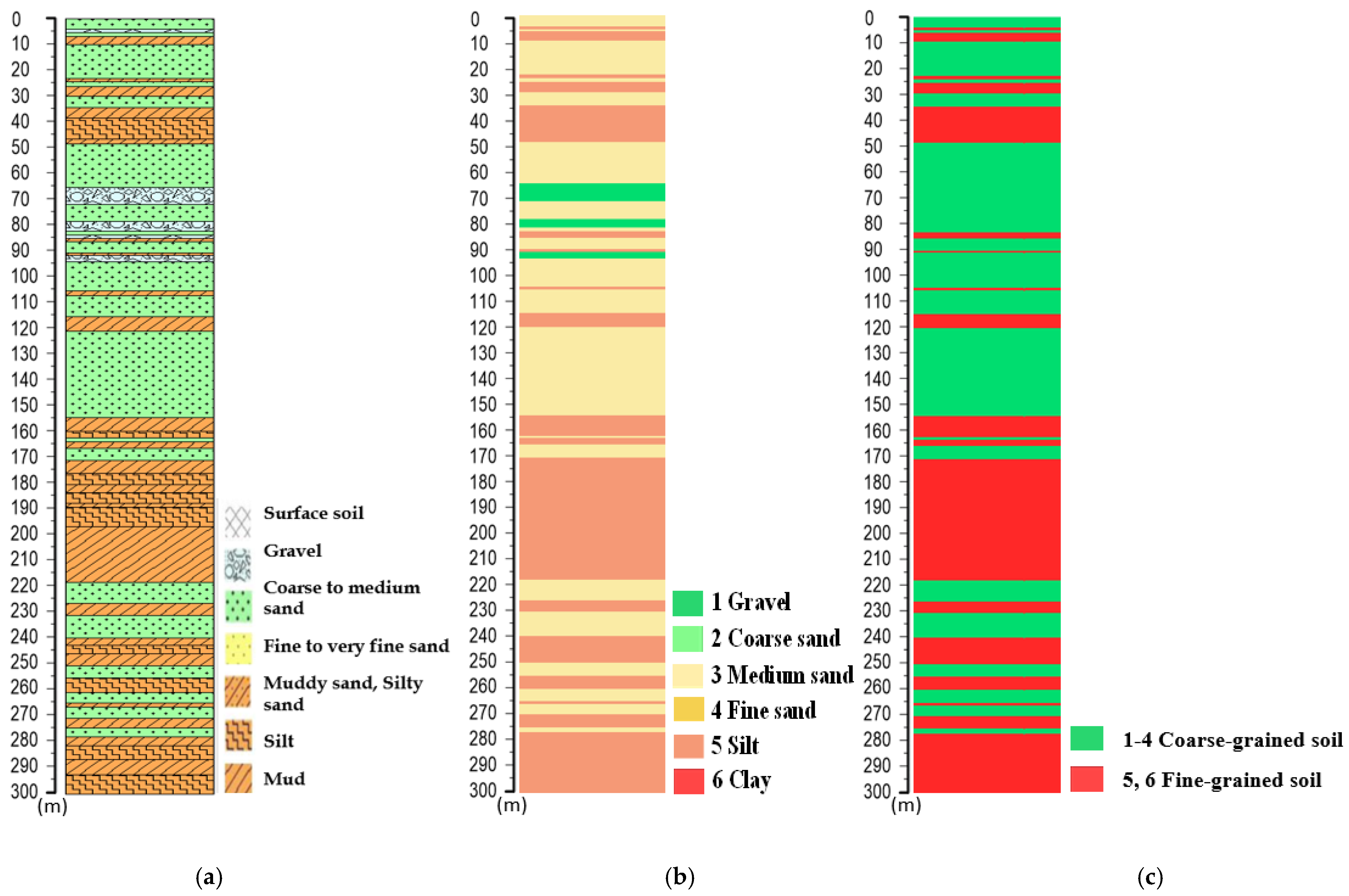
Using 75 borehole logging data from WRA and the CGS, we established the geological histogram, as demonstrated in Figure 3. Figure 3a illustrate examples of borehole logging data from WRA. Based on the soil classification as listed in Table 2, we classified the borehole logging data into six different soil type, as depicted in Figure 3b. The soil composition of the geological histogram was then used to classify and calculate the proportion of coarse-grained and fine-grained soils, as shown in Figure 3c. The coarse-grained soils were categorized as the aquifer. On the other hand, the fine-grained soils corresponded to the aquitard.
To evaluate the percentage of coarse-grained soil [29], we utilized the following equation.
S c = H c H t ,
where S c denotes the percentage of coarse-grained soil, H c denotes the soil thickness of coarse-grained soil, and H t denotes the total drilling depth.

2.2.2. Percentage of Fine-Grained Soil

According to the unified soil classification system, fine-grained soils are defined with 50% or more passing through the No. 200 sieve [30]. Particles of this size cannot usually be seen with the naked eye, even with the aid of a magnifying glass. Fine-grained soils contain three types of soils, including fine sand, silt, and clay, as listed in Table 2. The percentage of fine-grained soil is the ratio of the thickness of fine sand, silt, and clay to the total drilling depth.
Using same procedure as demonstrated in Figure 3, we evaluated the percentage of fine-grained soil using the following equation [31].
S f = H f H t ,
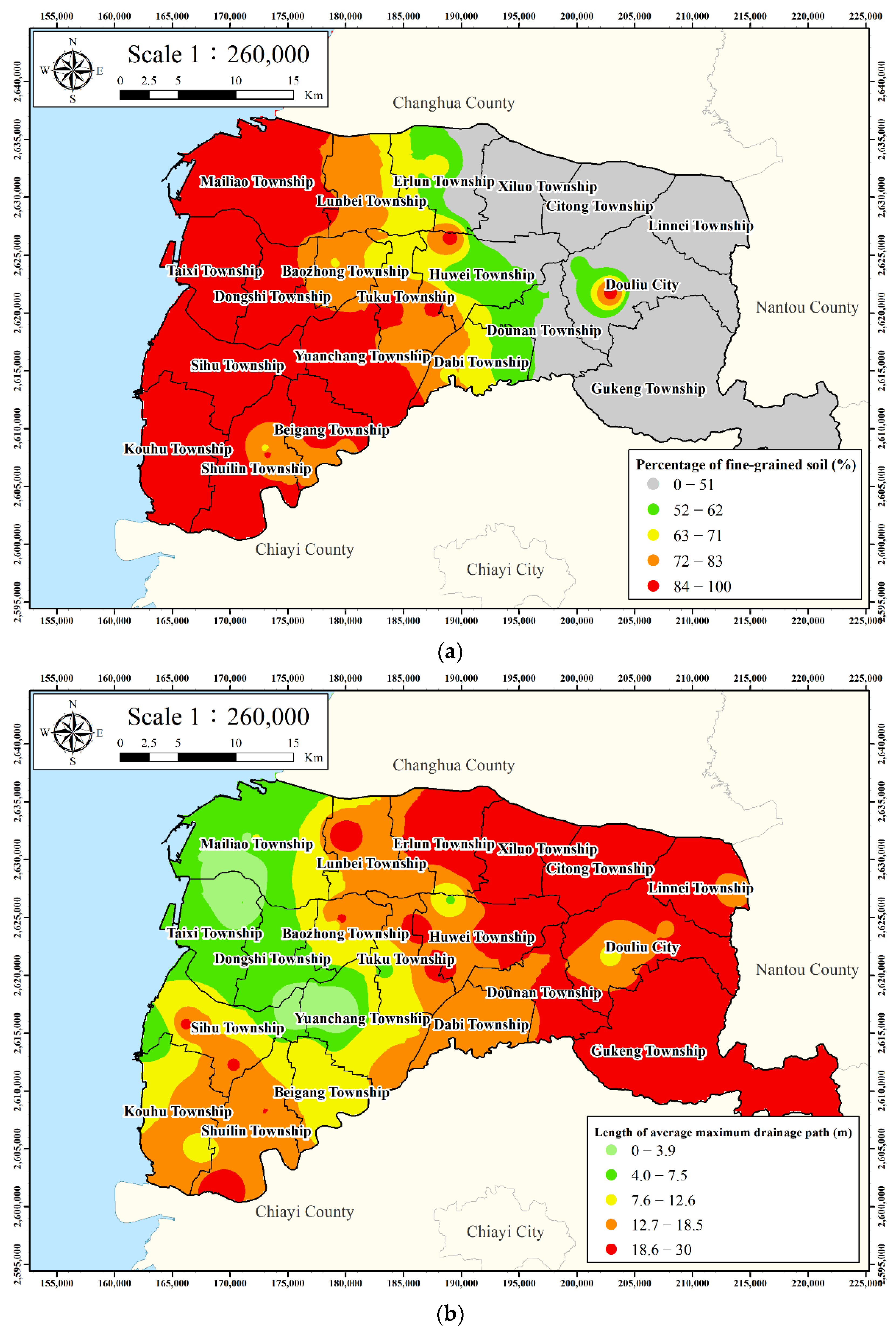
where S f denotes the percentage of fine-grained soil and H f denotes the soil thickness of fine-grained soil. Figure 2a shows the percentage of fine-grained soil of Yunlin County. According to Figure 2a, it is clear that the percentage of fine-grained soil in the near shore land zone of western Yunlin County is higher than that of the eastern Yunlin County.

2.2.3. Length of Average Maximum Drainage Path

When stress increases in a saturated soil layer, the pore water pressure suddenly increases. The reduction in the volume of the soil mass results in settlement. The settlement in clayey soil may be several times greater than the elastic settlement. The deformation of clayey soil can be described with the consideration of the length of the average maximum drainage path. Considering the top and bottom drainage conditions for the soil layer, the length of average maximum drainage path is defined as the average drainage path length, which can be expressed as follows [30].
H d r = 1 n i = 1 n ( H i f / 2 ) ,
where H d r denotes the length of the average maximum drainage path during compaction and H i f denotes the soil thickness of fine-grained soil. Figure 2b shows the length of the average maximum drainage path of Yunlin County. As demonstrated in Figure 2b, it is found that the length of average maximum drainage path in the near shore land zone of western Yunlin County is lower than that of the eastern Yunlin County.

2.2.4. Percentage of Agricultural Land Use

The thematic map of land use inventory of Yunlin County is illustrated in Figure 2c. The study area is classified into nine land use types, including agricultural land, forestry land, transportation land, hydrological land, construction land, public facility land, recreational land, mine industry land, and other regulation district [28], as depicted in Figure 2c. As demonstrated in Figure 2c, the land use in Yunlin County is mainly categorized as agriculture.
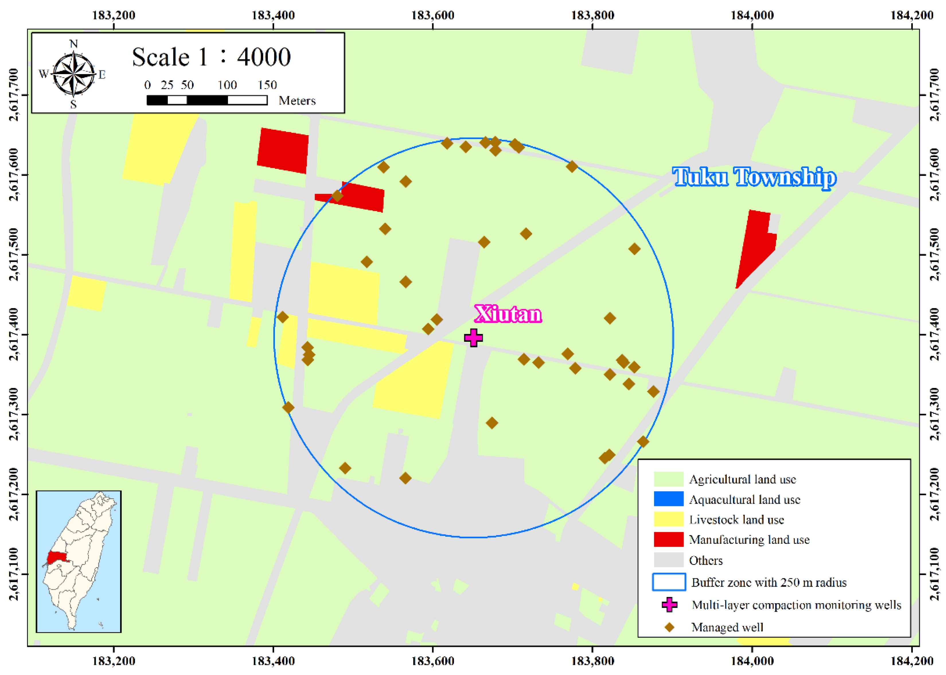
This study calculated the proportion of the agricultural land use within 250 m of each multi-layer compaction monitoring well (MLCW), as shown in Figure 4. The buffer analysis tool in ArcGIS creates buffer polygons around input features to a specified distance to adopt the spatial analysis and calculates the proportion of the agricultural land of the specified area. The percentage of agricultural land use is defined as follows.
L f = F a T a ,
where L f denotes percentage of agricultural land use, F a denotes area of agricultural land use in the division unit, and T a denotes total area of the unit.

2.2.5. Electricity Consumption of Wells

The electricity consumption of managed wells within a radius of 250 m for each MLCW was collected. Considering the agricultural use, the wells located at the depth of 0 to 60 m from 2015 to 2020 were filtered [26]. The point density tool in ArcGIS was adopted to calculate the density of features in a neighborhood around the features, to analyze the spatial electricity consumption of the managed wells of the area. The electricity consumption of the managed water wells per unit area was calculated as
W e = E T a ,
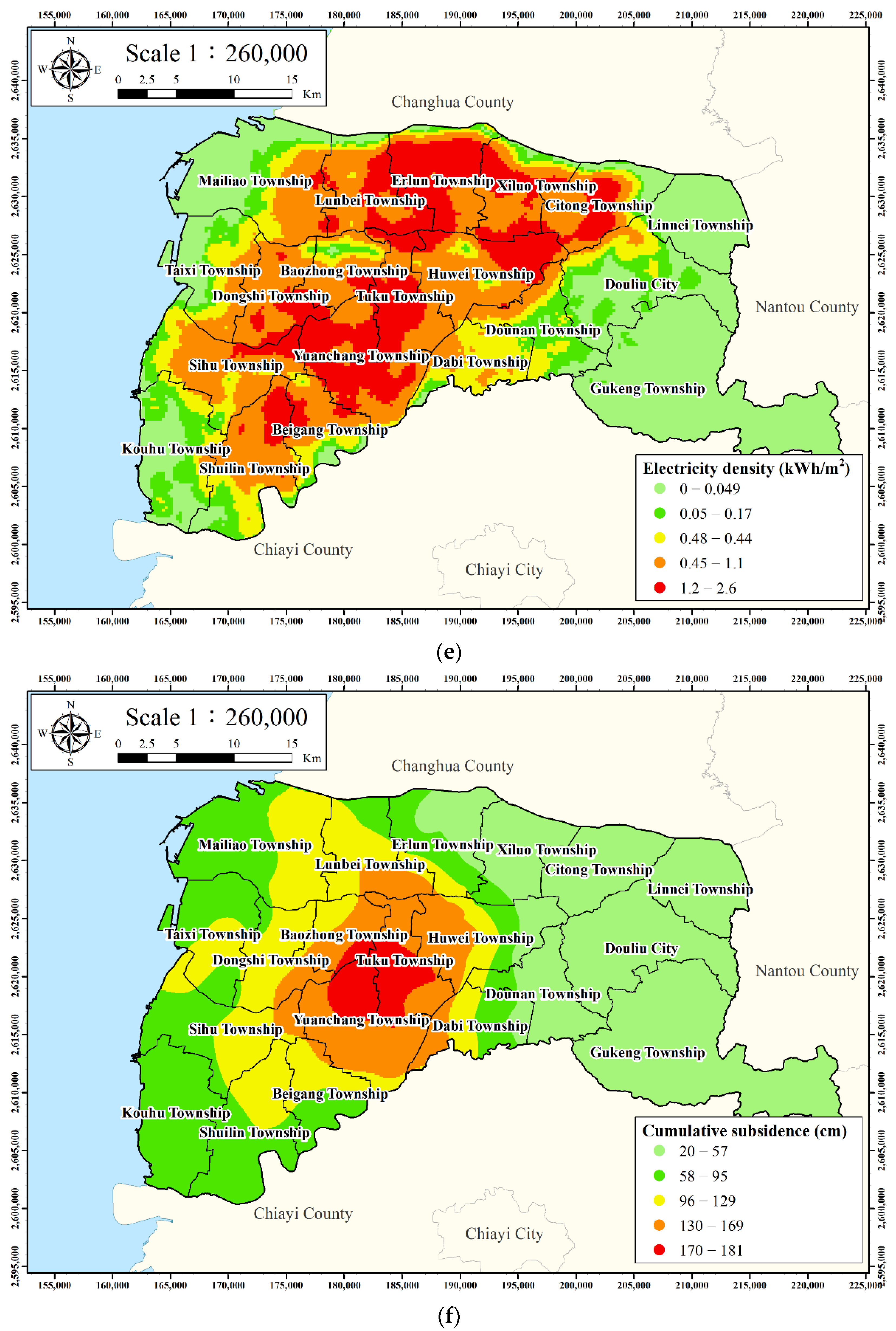
where W e denotes the electricity consumption of managed wells per unit area and E denotes the total electricity consumption of managed wells by division unit. Figure 2d,e illustrate the distribution of the managed wells and the electricity consumption of the managed wells of Yunlin County. According to Figure 2e, it is clear that the electricity consumption of the managed wells at the middle of Yunlin County is higher than that of the eastern and western Yunlin County.

2.2.6. Accumulated Subsidence Depth

The land subsidence in Yunlin County by levelling surveys ranging from 1992 to 2020 was used. The inverse distance weighting tool in ArcGIS was adopted to interpolate the land subsidence data to find the spatial and temporal subsidence characteristics in Yunlin County. According to Figure 2f, the most significant land subsidence area is situated in the Tuku Township and Yuanchang Township. The maximum accumulated subsidence depth reached 180 cm in the past thirty years from 1992 to 2020, as shown in Figure 2f.
However, the subsidence characteristics are significantly affected by the change in environmental impacts of groundwater in the inland and coastal areas. The characteristics and trends of land subsidence were slowed in the coastal areas, while the subsidence areas are mainly in inland areas in the past 10 years. The significant subsidence area is mainly located in the central area of the Choshui delta.

2.3. Principal Component Analysis

Since the data dimensionality can be evaluated by the independent variables, the PCA was used to observe a set of principal components that are linearly uncorrelated. The eigenvector satisfies
A x = x λ
where x denotes the input data, A denotes a matrix, and λ denotes a scalar. The left-hand side of Equation (6) transforms the input data x, and the right-hand side of Equation (6) scales the data by λ. The PCA for the dimensionality reduction can be carried out using the linear transformation as follows [32,33,34].
A w = w λ ,
y = w x ,
where w denotes the eigenvector (principal component), λ denotes the eigenvalues, and y denotes the transformed variable. The above equations [34,35] were rewritten as
A p × p w p × k = w p × k λ k × k ,
y k × n = w k × p x p × n ,
where n denotes the number of features. Utilizing Equations (9) and (10), the original data set were transformed from p to k dimensions, where kp. The features were reduced from p to k. Utilizing the principal components as the weights, the original input data x was transformed into y, as shown in Equation (10) [34,35,36]. Adopting the covariance matrix C, we can achieve
C p × p w p × k = w p × k λ k × k ,
y k × n = w k × p x p × n ,
where C is the covariance matrix, which is a symmetric square. The C matrix can be estimated as
C p × p = 1 n 1 x p × n x n × p .
If the dimensionality reduction is not required, Equations (11) and (12) can be rewritten as [36]:
C p × p w p × p = w p × p λ p × p ,
y p × n = w p × p x p × n .
The objective of the above equations is to deal with the eigenvector equations to estimate the eigenvectors and eigenvalues for a covariance matrix [36].

3. Results

This study utilized the PCA to investigate the dominant environmental factors affecting land subsidence [37,38,39]. In this study, five factors were considered as the dominant environmental factors for land subsidence as listed in Table 3. According to Table 3, the following factors include factor #1 (percentage of agricultural land use), factor #2 (electricity consumption of wells), factor #3 (percentage of fine-grained soil), factor #4 (length of maximum drainage path), and factor #5 (accumulation depth of land subsidence from 2015 to 2020).
Factor #1 was utilized by the survey results of the current state of land use from the NLSC, Ministry of the Interior. The proportion of the agricultural land use within 250 m of each MLCW was examined. Factor #2 was collected from the electricity consumption of the managed wells from the WRA. The electricity consumption of managed wells located at the depth of 0 to 60 m from 2015 to 2020 within a radius of 250 m centered on each MLCW was then calculated. Factors, including factor #3 and factor #4, were generated from the borehole data from the CGS and WRA of Taiwan. Factor #5 was collected from the WRA.
The PCA was used to analyze the environmental factors for land subsidence [37,38,39]. This study used the drilling data of 24 stratified subsidence monitoring wells (from the WRA) in Yunlin County, and the drilling data of 51 hydrogeological drilling wells (from the CGS) in Yunlin County. A total of 75 drilling wells were analyzed, where the average depth of the drilling wells was 200.75 m. This study calculated the environmental factors of each drilling well in the Yunlin County, and conducted a PCA to capture the relationship between each environmental factor and the land subsidence.
To examine the influence of different environmental factors on land subsidence, the correlation coefficient was first calculated. The results of the correlation coefficient matrix were then obtained to evaluate the correlation between the factors. Table 4 depicts the results of the correlation coefficient matrix. According to Table 4, factor #5 (accumulation depth of land subsidence from 2015 to 2020) is the cumulative subsidence factor, which is positively correlated with the factor #1 (percentage of agricultural land use), factor #2 (electricity consumption of wells), and factor #3 (percentage of fine-grained soil). The results obtained show that the correlation with factor #2 (electricity consumption of wells) is the highest, which is 0.46, indicating the high electricity consumption of the wells increase the accumulated land subsidence. Since the main diagonal is the correlation coefficient of the factor itself, the correlation coefficients were all 1, as listed in Table 4.
Table 5 shows the values of component loading in the PCA component matrix. According to Table 5, the loading of the factor in different principal components can be obtained to evaluate the correlation between the factor and the principal component (PC). Table 6 shows the eigenvalue and contribution table of the principal components. Each principal component has a certain degree of representativeness for the interpretation of the entire data, which is determined by the contribution rate. As depicted in Table 6, the eigenvalues and contribution rates of factors demonstrate that the cumulative contribution of the first two principal components is 64.06%. It was found that the first two principal components can explain 64% of the data, which is representative to a certain extent. The contribution is 93.31%, which means that the first four principal components can explain almost all the data.
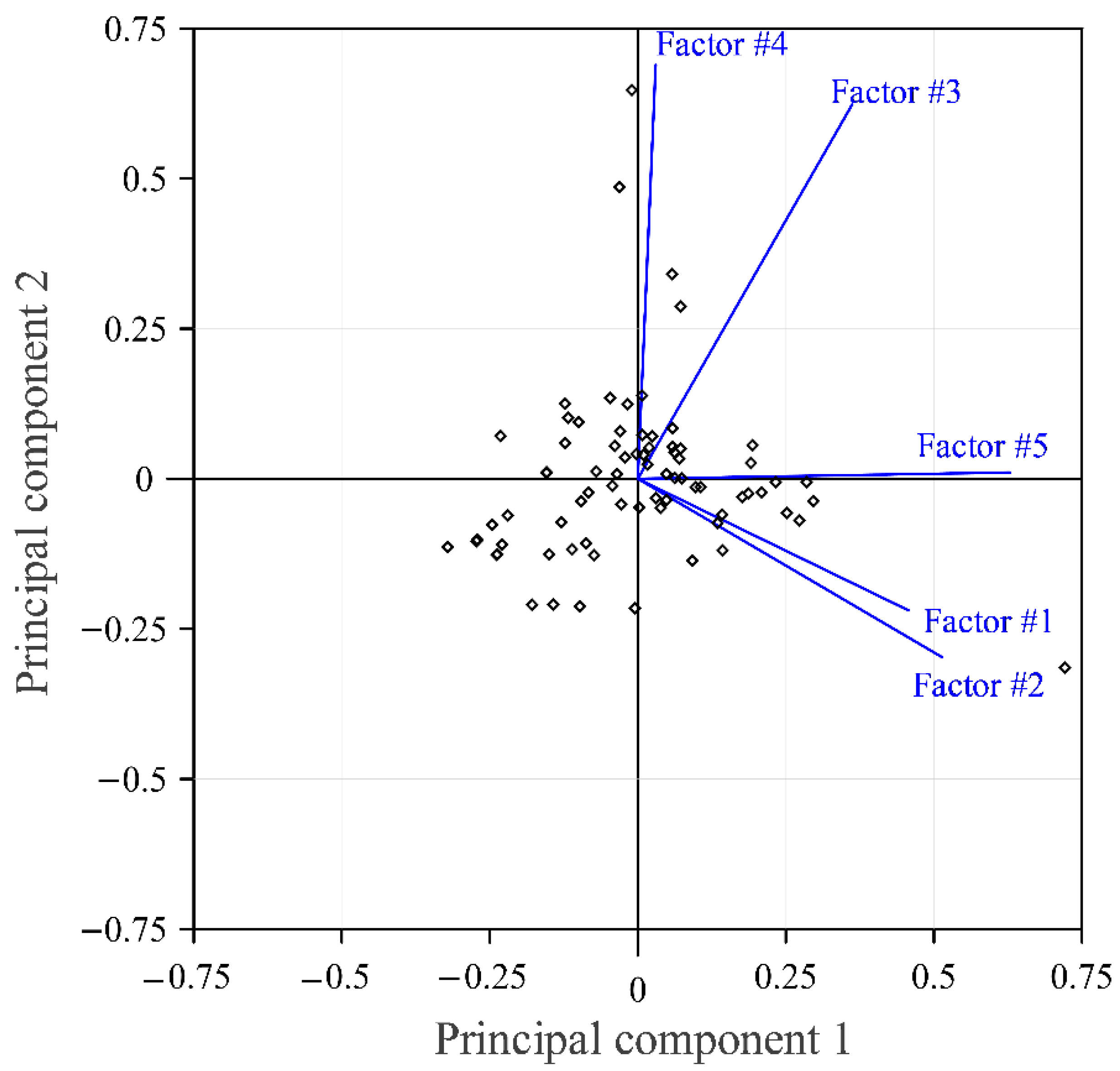
According to the loading of the first two principal components in Table 6, the distribution of principal components can then be analyzed. Figure 5 displays the distribution of the principal component. As shown in Figure 5, all factors utilized are positive on principal component 1. Among them, factor #1 (percentage of agricultural land use), factor #2 (electricity consumption of wells), and factor #5 (accumulation depth of land subsidence from 2015 to 2020) have higher loading in the first principal component. It appears that the first principal component is mainly based on the proportion of agricultural land use, electricity consumption of wells, and accumulated subsidence data, while other factors also show a positive correlation with the accumulated land subsidence. According to Figure 5, factor #3 (percentage of fine-grained soil) and factor #4 (length of average maximum drainage path) have a higher loading in the second principal component. It was found that the second principal component is more correlated with the length of average maximum drainage path in terms of fine aggregate content, which can also be obtained from Figure 5. The results obtained illustrate that the electricity consumption of the wells and the loading of the accumulated land subsidence on the first principal component are very similar, indicating that these two factors are highly correlated. The results of this example demonstrate that the electricity consumption of wells is highly correlated with the accumulated land subsidence. In addition, the first principal component can be explained as an acquired factor causing land subsidence, such as the excessive withdrawal of groundwater. In addition, the second principal component can be interpreted as the congenital factor causing land subsidence, that is, the data related to the characteristics of the soil layer. Since the electricity consumption of wells has the highest correlation with the accumulated subsidence, factor #5 (accumulation depth of land subsidence from 2015 to 2020) is closer to the first principal component in the distribution of the principal components, as shown in Figure 5.

4. Discussion

To investigate the dominant environmental factors affecting land subsidence in Yunlin County, this study used principal component analysis to analyze five factors, i.e., factor #1, factor #2, factor #3, factor #4, and factor #5. Based on the PCA results, the first principal component can be interpreted as the data related to the pumping behavior, and the second principal component can be interpreted as the soil layer. The cumulative subsidence has the highest correlation with electricity consumption, and is also distributed on the first principal component. Furthermore, the results indicate that the largest subsidence rate is observed within the region that has both a high electricity consumption of wells and a large percentage of fine-grained soil. The PCA results reveal that the electricity consumption of wells is highly correlated with the accumulated depth of land subsidence. The first principal component is the acquired factor causing land subsidence, such as the excessive withdrawal of groundwater. The second principal component is the congenital factor causing land subsidence, which corresponds to fine sand, silty, and clayey soils.
The proposed method, based on GIS spatial analysis and PCA, can characterize land subsidence with the spatial variability of soil formation and groundwater withdrawals and present results in a spatial environment in the Choshui delta, Taiwan. The main advantage of the GIS spatial analysis capability is integrated into the PCA. Accordingly, the proposed approach may represent spatial continuity and the investigation of the dominant environmental factors for characterizing of land subsidence. However, the purpose of the PCA adopted in this study may only limited to evaluate the inter-correlations among variables

5. Conclusions

This study presented the characterization of land subsidence with the spatial variability of soil formation and groundwater withdrawals in the Choshui delta, Taiwan. Various factors, including the percentage of coarse-grained soil, percentage of fine-grained soil, length of maximum drainage path, percentage of agricultural land use, electricity consumption of wells, and accumulated depth of land subsidence, were adopted. The thematic maps based on these factors were established utilizing the GIS spatial analysis. The fundamental concepts and construct of the proposed method were addressed in detail. The findings are as follows:
  • To examine the influence of different environmental factors on land subsidence, the correlation coefficient was calculated. The results obtained show that factor #5 (accumulation depth of land subsidence from 2015 to 2020) is the cumulative subsidence factor, which is positively correlated with factor #1 (percentage of agricultural land use), factor #2 (electricity consumption of wells), and factor #3 (percentage of fine-grained soil). Furthermore, it was found that the correlation with factor #2 (electricity consumption of wells) is the highest, which is 0.46, indicating the high electricity consumption of the wells increases the accumulated land subsidence.
  • The eigenvalues and contribution rates of factors demonstrate that the cumulative contribution of the first two principal components is 64.06%. It is found that the first two principal components can explain 64% of the data, which is representative to a certain extent. The contribution is 93.31%, which means that the first four principal components can explain almost all the data.
  • From the PCA results, the largest subsidence rate was observed within the region that has both a high electricity consumption of wells and a large percentage of fine-grained soil. It appears that the electricity consumption of wells is highly correlated with the accumulated depth of land subsidence. The first principal component is the acquired factor causing land subsidence, such as the excessive withdrawal of groundwater. The second principal component is the congenital factor causing land subsidence, which corresponds to fine sand, silty, and clayey soils. The findings observed in this study may provide authorities with more information for planning future mitigation measures in significant land subsidence areas.

Author Contributions

Conceptualization, C.-Y.K.; Performed the analysis, C.-Y.L.; Data collection, H.-C.L.; Writing, C.-Y.K. and C.-Y.L.; All authors have read and agreed to the published version of the manuscript.

Funding

This study was supported by the National Science Council, Taiwan, The Republic of China (MOST 111-MOEA-M-008-001).

Institutional Review Board Statement

Not applicable.

Informed Consent Statement

Not applicable.

Data Availability Statement

The datasets generated during the current study are available from the corresponding authors upon reasonable request.

Conflicts of Interest

The authors declare no conflict of interest.

References

  1. Faunt, C.C.; Sneed, M.; Traum, J.; Brandt, J.T. Water availability and land subsidence in the Central Valley, California, USA. Hydrogeol. J. 2016, 24, 675–684. [Google Scholar] [CrossRef] [Green Version]
  2. Sneed, M.; Galloway, D.L. Aquifer-System Compaction and Land Subsidence: Measurements, Analyses, and Simulations: The Holly Site, Edwards Air Force Base; (No. 4015); US Department of the Interior, US Geological Survey: Antelope Valley, CA, USA, 2000. [Google Scholar]
  3. Pang, S.C.; Yeh, T.K.; Hong, J.S.; Chen, C.H. Variability and climatology of precipitable water vapor from 12-year GPS observations in Taiwan. Adv. Space Res. 2021, 67, 2333–2346. [Google Scholar] [CrossRef]
  4. Ku, C.Y.; Liu, C.Y.; Su, Y.; Xiao, J.E.; Huang, C.C. Transient modeling of regional rainfall-triggered shallow landslides. Environ. Earth Sci. 2017, 76, 570. [Google Scholar] [CrossRef]
  5. Khoirunisa, N.; Ku, C.Y.; Liu, C.Y. A GIS-based artificial neural network model for flood susceptibility assessment. Int. J. Environ. Res. Public Health 2021, 18, 1072. [Google Scholar] [CrossRef]
  6. Liu, C.H.; Pan, Y.W.; Liao, J.J.; Huang, C.T.; Ouyang, S. Characterization of land subsidence in the Choshui River alluvial fan, Taiwan. Eng. Geol. 2004, 45, 1154–1166. [Google Scholar]
  7. Hung, W.C.; Hwang, C.; Chang, C.P.; Yen, J.Y.; Liu, C.H.; Yang, W.H. Monitoring severe aquifer-system compaction and land subsidence in Taiwan using multiple sensors: Yunlin, the southern Choushui River Alluvial Fan. Environ. Earth Sci. 2010, 59, 1535–1548. [Google Scholar] [CrossRef]
  8. Hung, W.C.; Hwang, C.; Liou, J.C.; Lin, Y.S.; Yang, H.L. Modeling aquifer-system compaction and predicting land subsidence in central Taiwan. Eng. Geol. 2012, 147, 78–90. [Google Scholar] [CrossRef]
  9. Castellazzi, P.; Arroyo-Domínguez, N.; Martel, R.; Calderhead, A.I.; Normand, J.C.; Gárfias, J.; Rivera, A. Land subsidence in major cities of Central Mexico: Interpreting InSAR-derived land subsidence mapping with hydrogeological data. Int. J. Appl. Earth Obs. Geoinf. 2016, 47, 102–111. [Google Scholar] [CrossRef]
  10. Qiao, X.; Chu, T.; Tissot, P.; Louis, J.; Ali, I. Land subsidence estimation with tide gauge and satellite radar altimetry measurements along the Texas Gulf Coast, USA. IEEE Geosci. Remote Sens. Lett. 2022, 19, 1–5. [Google Scholar] [CrossRef]
  11. Li, A.; Tsai, F.T.C.; Yuill, B.T.; Wu, C. A three-dimensional stratigraphic model of the Mississippi River Delta, USA: Implications for river deltaic hydrogeology. Hydrogeol. J. 2020, 28, 2341–2358. [Google Scholar] [CrossRef]
  12. Zhang, Y.; Gong, H.; Gu, Z.; Wang, R.; Li, X.; Zhao, W. Characterization of land subsidence induced by groundwater withdrawals in the plain of Beijing city, China. Hydrogeol. J. 2014, 22, 397–409. [Google Scholar] [CrossRef]
  13. Smith, R.G.; Majumdar, S. Groundwater storage loss associated with land subsidence in Western United States mapped using machine learning. Water Resour. Res. 2020, 56, e2019WR026621. [Google Scholar] [CrossRef]
  14. Liu, C.; Shi, B.; Gu, K.; Zhang, T.; Tang, C.; Wang, Y.; Liu, S. Negative pore water pressure in aquitard enhances land subsidence: Field, laboratory, and numerical evidence. Water Resour. Res. 2022, 58, e2021WR030085. [Google Scholar] [CrossRef]
  15. Budhu, M.; Adiyaman, I. The influence of clay zones on land subsidence from groundwater pumping. Groundwater 2013, 51, 51–57. [Google Scholar] [CrossRef] [PubMed]
  16. Zhou, G.; Esaki, T.; Mori, J. GIS-based spatial and temporal prediction system development for regional land subsidence hazard mitigation. Environ. Geol. 2003, 44, 665–678. [Google Scholar] [CrossRef]
  17. Antonellini, M.; Giambastiani, B.M.S.; Greggio, N.; Bonzi, L.; Calabrese, L.; Luciani, P.; Perini, L.; Severi, P. Processes governing natural land subsidence in the shallow coastal aquifer of the Ravenna coast, Italy. Catena 2019, 172, 76–86. [Google Scholar] [CrossRef]
  18. Chu, H.J.; Lin, C.W.; Burbey, T.J.; Ali, M.Z. Spatiotemporal analysis of extracted groundwater volumes estimated from electricity consumption. Groundwater 2020, 58, 962–972. [Google Scholar] [CrossRef]
  19. Peng, Y.; Dong, D.; Chen, W.; Zhang, C. Stable regional reference frame for reclaimed land subsidence study in East China. Remote Sens. 2022, 14, 3984. [Google Scholar] [CrossRef]
  20. Xiao, B.; Zhao, J.; Li, D.; Zhao, Z.; Xi, W.; Zhou, D. The monitoring and analysis of land subsidence in Kunming (China) supported by time series InSAR. Sustainability 2022, 14, 12387. [Google Scholar] [CrossRef]
  21. Larson, K.J.; Başaǧaoǧlu, H.; Marino, M.A. Prediction of optimal safe ground water yield and land subsidence in the Los Banos-Kettleman City area, California, using a calibrated numerical simulation model. J. Hydrol. 2001, 242, 79–102. [Google Scholar] [CrossRef]
  22. Leake, S.A.; Galloway, D.L. Use of the SUB-WT Package for MODFLOW to simulate aquifer-system compaction in Antelope Valley, California, USA. In Land Subsidence, Associated Hazards and the Role of Natural Resources Development, Proceedings of the Eighth International Symposium on Land Subsidence, Queretaro, Mexico, 17–22 October 2010; International Association of Hydraulic Sciences: Queretaro, Mexico, 2010; pp. 61–67. [Google Scholar]
  23. Nadiri, A.A.; Habibi, I.; Gharekhani, M.; Sadeghfam, S.; Barzegar, R.; Karimzadeh, S. Introducing dynamic land subsidence index based on the ALPRIFT framework using artificial intelligence techniques. Earth Sci. Inform. 2022, 15, 1007–1021. [Google Scholar] [CrossRef]
  24. Nadiri, A.A.; Moazamnia, M.; Sadeghfam, S.; Barzegar, R. Mapping Risk to Land Subsidence: Developing a Two-Level Modeling Strategy by Combining Multi-Criteria Decision-Making and Artificial Intelligence Techniques. Water 2021, 13, 2622. [Google Scholar] [CrossRef]
  25. Sadeghfam, S.; Nourbakhsh Khiyabani, F.; Khatibi, R.; Daneshfaraz, R. A study of land subsidence problems by ALPRIFT for vulnerability indexing and risk indexing and treating subjectivity by strategy at two levels. J. Hydroinform. 2020, 22, 1640–1662. [Google Scholar] [CrossRef]
  26. Water Resources Agency, Ministry of Economic Affairs. Available online: https://data.gov.tw/dataset/41572 (accessed on 1 June 2022). (In Chinese)
  27. Central Geological Survey. Available online: https://geotech.moeacgs.gov.tw/imoeagis/Home/Supply (accessed on 1 June 2022). (In Chinese)
  28. National Land Surveying and Mapping Center (NLSC), Ministry of the Interior. Available online: https://maps.nlsc.gov.tw/homePage.action?in_type=mobile (accessed on 1 June 2022). (In Chinese)
  29. Indrawan, I.G.B.; Rahardjo, H.; Leong, E.C. Effects of coarse-grained materials on properties of residual soil. Eng. Geol. 2006, 82, 154–164. [Google Scholar] [CrossRef]
  30. Das, B.M. Principles of Geotechnical Engineering; Cengage Learning: Boston, MA, USA, 2011. [Google Scholar]
  31. Sridharan, A.; Gurtug, Y. Swelling behaviour of compacted fine-grained soils. Eng. Geol. 2004, 72, 9–18. [Google Scholar] [CrossRef]
  32. Daffertshofer, A.; Lamoth, C.J.; Meijer, O.G.; Beek, P.J. PCA in studying coordination and variability: A tutorial. Clin. Biomech. 2004, 19, 415–428. [Google Scholar] [CrossRef] [PubMed]
  33. Linhai Jing, Q.C.; Panahi, A. Principal component analysis with optimum order sample correlation coefficient for image enhancement. Int. J. Remote Sens. 2006, 27, 3387–3401. [Google Scholar] [CrossRef]
  34. Schober, P.; Boer, C.; Schwarte, L.A. Correlation coefficients: Appropriate use and interpretation. Anesth. Analg. 2018, 126, 1763–1768. [Google Scholar] [CrossRef]
  35. Suthaharan, S. Machine learning models and algorithms for big data classification. Integr. Ser. Inf. Syst 2016, 36, 1–12. [Google Scholar]
  36. Kreyszig, E. Advanced Engineering Mathematics; John Wiley and Sons, Inc.: New York, NY, USA, 2008. [Google Scholar]
  37. Wang, Y.; Fan, Y.; Wang, Q.; Zhang, S.; Shi, Y.; Zheng, X. Response of Soil Fertility and Bacterial Community Composition to Vegetation Species in a Coal Mining Subsidence Area: A Survey After 20-Year Reclamation. Front. Environ. Sci. 2022, 10, 937688. [Google Scholar] [CrossRef]
  38. Shi, L.; Gong, H.; Chen, B.; Zhou, C. Land Subsidence Prediction Induced by Multiple Factors Using Machine Learning Method. Remote Sens. 2020, 12, 4044. [Google Scholar] [CrossRef]
  39. Hu, B.; Zhang, J.; Na, J.; Liu, D.; Xie, G. Temporal principal component analysis and synthetic aperture radar interference analysis of the spatial and temporal evolution of ground subsidence in the Los Angeles area. J. Appl. Remote Sens. 2022, 16, 044504. [Google Scholar] [CrossRef]
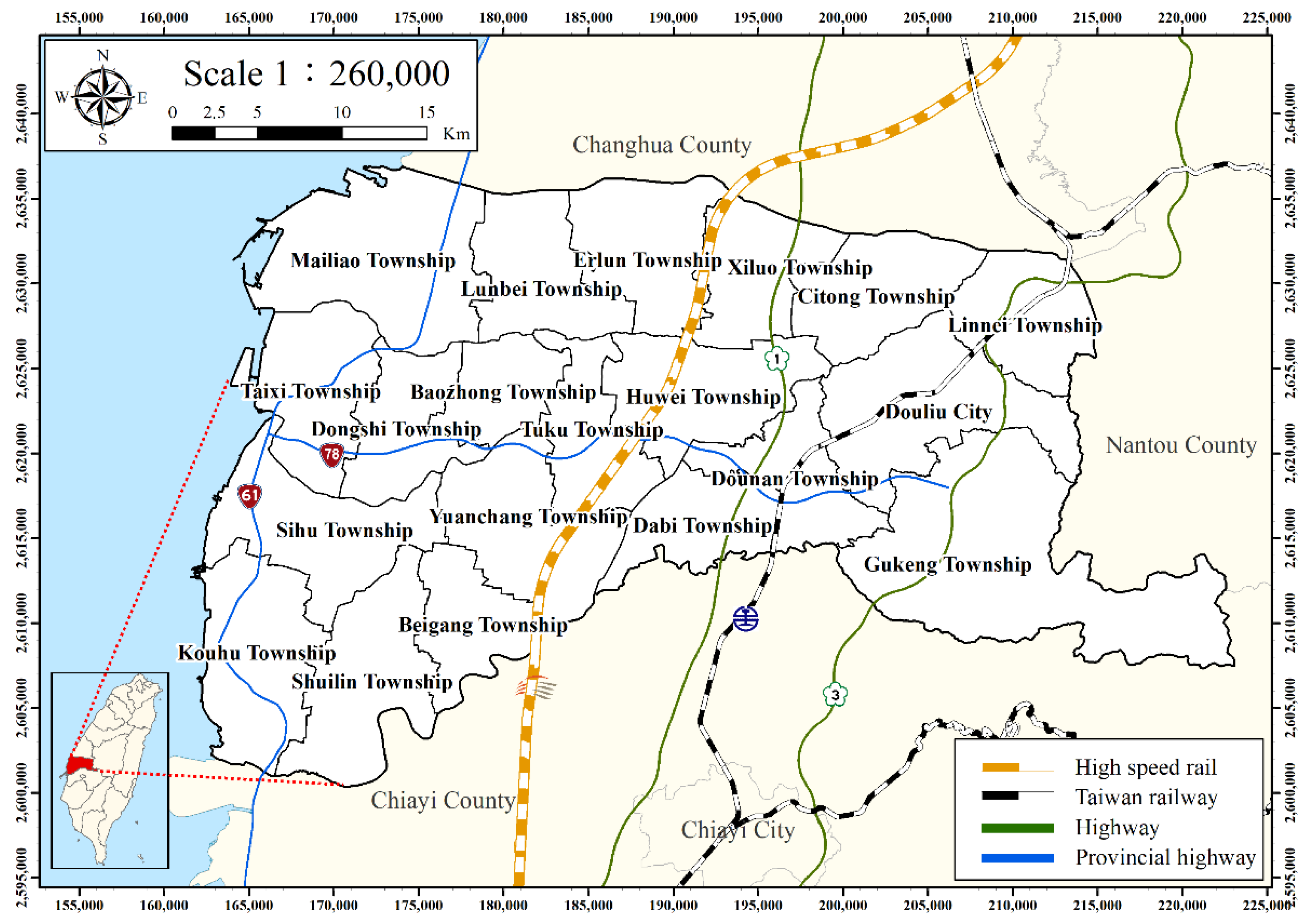
Figure 1. Administration map of Yunlin County, Taiwan.
Applsci 12 12464 g001
Figure 2. Thematic maps of Yunlin County, Taiwan, and relevant factors: (a) percentage of fine-grained soil; (b) length of average maximum drainage path; (c) percentage of agricultural land use; (d) distribution of the managed wells; (e) electricity consumption of wells; and (f) accumulated subsidence depth from 1992 to 2020.
Applsci 12 12464 g002aApplsci 12 12464 g002bApplsci 12 12464 g002c
Figure 3. Examples of borehole logging data: (a) Water Resources Agency; (b) this study (six soil type); (c) this study (two main type).
Applsci 12 12464 g003
Figure 4. The buffer analysis tool in ArcGIS.
Applsci 12 12464 g004
Figure 5. Plot of the factors in the principal components.
Applsci 12 12464 g005
Table 1. The source data used in this study [26,27,28].
No.FactorsSource Data
1Percentage of coarse-grained soilBorehole data from the CGS and WRA of Taiwan
2Percentage of fine-grained soil
3Length of average maximum drainage pathBorehole data from the CGS and WRA
4Percentage of agricultural land useLand use data from the NLSC
5Electricity consumption of wellsElectricity consumption data from the WRA
6Accumulated subsidence depthLand subsidence data from the WRA
Table 2. Soil classification from the Water Resources Agency [26].
Soil PropertiesSoil TypeClassificationMain Type
Gravel and coarse gravelGravel1Coarse-grained soil (Aquifer)
Grey coarse sand and coarse sandCoarse sand2
Coarse to medium sand and medium sandMedium sand3
Grey silty sand, grey fine sand, blue-gray silty sand, and fine to very fine sandFine sand4
Mud, muddy sand, sandy mud,
silty sand, surface soil, silt, backfill sand,
brown-gray sandy silt, and grey sandy silt
Silt5Fine-grained soil (Aquitard)
Grey silty clay, grey clay, and clayClay6
Table 3. The dominant environmental factors for land subsidence in this study.
No.FactorsData Source
1Percentage of agricultural land useLand use data from the NLSC
2Electricity consumption of wellsElectricity consumption data from the WRA
3Percentage of fine-grained soilBorehole data from the CGS and WRA
4Length of average maximum drainage pathBorehole data from the CGS and WRA
5Accumulation depth of land subsidence from 2015 to 2020Land subsidence data from the WRA
Table 4. The covariance matrix.
Factor
12345
Factor11.000.310.06−0.040.33
20.311.000.02−0.080.46
30.060.021.000.340.41
4−0.04−0.080.341.00−0.06
50.330.460.41−0.061.00
Table 5. The values of component loading in the PCA component matrix.
No.Factor DefinitionPC 1PC 2PC 3PC 4
Factor #1Percentage of agricultural land use0.46−0.220.67−0.54
Factor #2Electricity consumption of wells0.51−0.300.070.71
Factor #3Percentage of fine-grained soil0.360.62−0.33−0.26
Factor #4Length of average maximum drainage path0.030.690.540.37
Factor #5Accumulation depth of land subsidence from 2015 to 20200.630.01−0.38−0.06
Table 6. Rates of principal components.
EigenvalueRate of Contribution (%)Cumulative Contribution (%)
Principal component 11.8537.0037.00
Principal component 21.3527.0564.06
Principal component 30.7815.6779.73
Principal component 40.6813.5893.31
Publisher’s Note: MDPI stays neutral with regard to jurisdictional claims in published maps and institutional affiliations.