Article

Characteristics of Local Geomagnetic Field Variations and the Tectonic Stress Field Adjacent to the 21 May 2021, Ms 6.4 Yangbi Earthquake, Yunnan, China

1
Institute of Geophysics, China Earthquake Administration, Beijing 100081, China
2
Yunnan Earthquake Agency, Kunming 650224, China
3
Lanzhou Institute of Earthquake Research, China Earthquake Administration, Lanzhou 730000, China
4
Hebei Earthquake Agency, Shijiazhuang 050021, China
*
Authors to whom correspondence should be addressed.
Appl. Sci. 2022, 12(3), 1005; https://doi.org/10.3390/app12031005
Submission received: 24 November 2021 / Revised: 15 January 2022 / Accepted: 17 January 2022 / Published: 19 January 2022

Abstract

:

Featured Application

This work is mainly applied to the analysis of relevant geophysical field changes caused by earthquakes.

Abstract

The tectonic processes leading up to an earthquake and the occurrence of the earthquake itself will cause local changes in the geophysical field (geomagnetic field, stress field, etc.). In this paper, the variation characteristics of the tectonic stress field (TSF) and local geomagnetic field (LGF) before and after the Yangbi Ms 6.4 earthquake are studied. The regional stress tensor damping inversion method was used to invert the TSF using focal mechanism solutions (FMSs). The change characteristics of the TSF before and after the earthquake were analyzed. An annual variation model of the LGF was constructed, and the variation of the horizontal vector was analyzed. The azimuth and plunge of the maximum principal compressive stress axis of the TSF in the epicentral region before and after the earthquake were −4.4° and 2.7°, 172.7° and 6.6°, respectively. The variations in the declination, inclination and total intensity of the epicenter one year before and one month after the earthquake were −0.20′ (0.07′), 0.29′ (−0.12′), and −1.7 nT (−1.9 nT), respectively. The epicenter is located at the boundary of the “weak variation region” of the horizontal vector. This research is of great significance concerning the TSF background and incubation mechanism of earthquakes.

1. Introduction

The geomagnetic field and stress field are important geophysical fields. Changes in these fields caused by tectonic activities such as earthquakes have long been central issues in geophysical research [1,2]. Because these fields are associated with two different disciplines, little research on the relationship between the geomagnetic field and the stress field has been published [3,4].
Most earthquakes are processes of crustal stress release, which causes changes in the stress field on or around the fault, and has a great impact on the seismic activity in the area near the earthquake source [5]. The inversion of the tectonic stress field (TSF) based on the earthquake focal mechanism solution (FMS) is an effective method to study the process and mechanism of earthquake initiation and occurrence [6,7]. Although the FMS of a single earthquake cannot be used to define the actual direction of the tectonic stress applied underground, the characteristics of the TSF in the region can be inferred through many FMSs in a given area [8,9,10].
The lithospheric magnetic field, also known as the crustal magnetic field, is an important part of the geomagnetic field [11,12]. The spatial structure of lithospheric magnetic anomalies is extremely complex but very stable over time because the sources of the local geomagnetic field (LGF) are stable [13,14]. However, during strong tectonic activity, the LGF changes rapidly; examples of this include the magnetic field near earthquake buildup areas, volcanoes and faults [15,16,17]. Studies have shown that tectonic activities in the crust are related to changes in crustal stress [18,19]. The magnetic mineral composition of crustal rocks at temperatures below the Curie point shows the characteristics of induced magnetization and residual magnetization [20,21,22]. In the area of tectonic movement, these magnetic minerals produce local geomagnetic anomalies due to the piezomagnetic variations caused by stress [23,24,25]. How then does tectonic movement cause changes in the crustal stress, which, in turn, lead to variations in local geomagnetic anomalies [26,27]?
The corresponding relationship between the stress and the magnetic changes in rock samples has been established under laboratory conditions [28,29]. Based on laboratory results, many researchers have provided reasonable explanations for the magnetic anomalies caused by tectonic activity in the crust [18,30,31]. However, some researchers have also found that the magnetic anomalies observed during earthquakes are much smaller than expected. The expected magnetic changes are not observed in volcanic areas or near active faults, and even the magnetic changes observed during the storage of a reservoir are much larger than the calculated values based on the experimental conclusions [19,32]. The reason is that the results of magnetic experiments on rock samples have certain limitations. Due to the limitation of experimental conditions, the experimental environment of rock samples is often quite different from the underground physical environment in an area with geological tectonic movement, and the scale of rock samples is very different from that of a tectonic area [4,25]. The magnetic anomalies caused by general geological processes are difficult to explain based on conclusions from rock magnetic experiments.
There are no reports on the correlation between the TSF and LMF caused by earthquakes. On May 21, 2021, a magnitude 6.4 earthquake occurred in Yangbi County, Yunnan Province, China [33]. To better understand the tectonic stress background and the magnetic anomaly changes resulting from the earthquake, we used the fault sliding direction to reverse the TSF in the epicentral area and then analyzed the changes in the TSF before and after the Yangbi earthquake. At the same time, repeated observations of the geomagnetic field were used to analyze the changes in the LGF before and after the Yangbi earthquake. A “weak variation” pattern of the horizontal vector change in the epicentral area was revealed, and the evolution of the Yangbi earthquake was analyzed based on the experimental theory of meta-instability [34].

2. Data and Methods

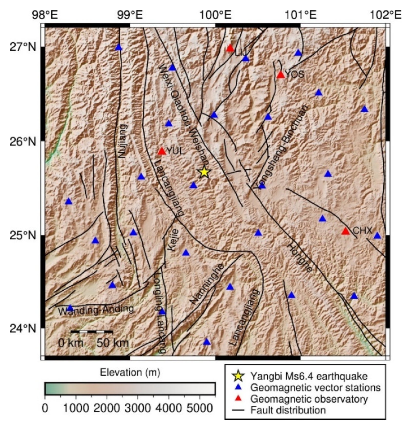
2.1. Yangbi Ms 6.4 Earthquake

The epicenter of the Ms 6.4 Yangbi earthquake was located at 99.87° E, 25.67° N, and the focal depth was 8 km (https://www.cea-igp.ac.cn/kydt/278248.html (accessed on 16 January 2022)), as shown in Figure 1. The earthquake sequence presents a typical foreshock-mainshock-aftershock pattern, which is roughly distributed in a NW strip along the western side of the Weixi-Qiaohou-Weishan fault [35]. The rupture featured a NW-SE high dip angle and right-handed strike-slip motion. The extreme slip zone was located southeast of the epicenter, and the main fracture length was approximately 12–15 km [33].

2.2. Inversion and Modeling Data

2.2.1. FMS Data

With the inversion of the TSF before the Yangbi earthquake, 40 FMSs with Mw > 4.8 from 1 January 1976 to 30 April 2021 were collected for the surrounding area (98° E−102° E, 23.7° N−27.2° N). These data were from the Global Centroid Moment Tensor Catalog (GCMT) of Harvard University. The focal mechanisms of these earthquakes show that the focal types in the study area are mainly strike-slip [37,38].
We used 13 earthquake events (Ms > 4.0) within 15 km of the epicentral area before and after the Yangbi earthquake to study the changes in the regional TSF. FMSs are shown in Table 1 [35].

2.2.2. Geomagnetic Measurement Data

There are four continuously recording geomagnetic observatories within 200 km of the mainshock. The nearest station (YUL) is only 55 km away from the epicenter, while the farthest (CHX)- is 180 km away. These stations are shown in the red triangles in Figure 1. These geomagnetic observatories provide reliable data for the correction of the daily variation and secular variation of the ground repeated magnetic survey data.
In addition, there are 27 repeated geomagnetic field vector measurement stations within 250 km of the epicenter, with a spacing of approximately 70 km (shown as blue triangles in Figure 1). The total intensity (F) of the geomagnetic field was measured using a proton precession magnetometer (GSM-19T) with an absolute accuracy of ± 0.2 nT and a resolution of 0.01 nT [4,25]. A DI magnetometer with an accuracy of 0.2′ and a resolution of 0.1′ was used to measure the magnetic inclination (I) [39]. GPS and DI magnetometer were combined to complete the measurement of the magnetic declination (D). These stations have recorded data from March to May every year since 2010.
In this paper, we use continuously recorded data from four observatories from 1 January 2018 to 30 June 2021, as well as a total of five ground magnetic vector observation data points during 2018–2021 and one month after the Yangbi earthquake.

2.3. Inversion and Modeling Methods

2.3.1. TSF Inversion Method

The regional stress tensor damping inversion method is adopted, and the damping coefficient is introduced based on the linear stress inversion method to control the mismatch between the theoretical and observed values and the relative weight of the model complexity [40]. First, the optimal damping coefficient in the inversion process is determined by an automatic program. Second, the FMSs are divided into many grids (each grid adopts at least one FMS), and stress inversion is carried out to obtain the optimal stress tensor for each grid point. Finally, the bootstrap method is used to resample the data of each grid to obtain the confidence interval of the stress tensor axis [41].
In this paper, the tectonic stress field near the epicenter is calculated by using the regional stress tensor damping inversion method and MSATSI program [42]. The number of earthquakes in every grid is set to 1, the number of automatic resamplings is 1000, and the confidence level is 95%.

2.3.2. LGF Modeling Method

According to the continuous absolute value data of the geomagnetic observatories (as shown in Figure 1), the diurnal variation of the observed data is corrected to eliminate the external field component of the geomagnetic field using the data processing method described by Wang et al. [25,43]. The secular variation of the geomagnetic field is eliminated by using the natural orthogonal component model in mainland China [4]. The 8th-order spherical cap harmonic model of the Chinese geomagnetic reference field is used to eliminate the main magnetic field component to obtain the lithospheric magnetic field change every year, and then the lithospheric magnetic field of the adjacent two years is used to obtain the annual change [39]. Finally, the surface spline fitting method is used to construct a high-precision model of the annual change in the lithospheric magnetic field in the study area.

3. Results

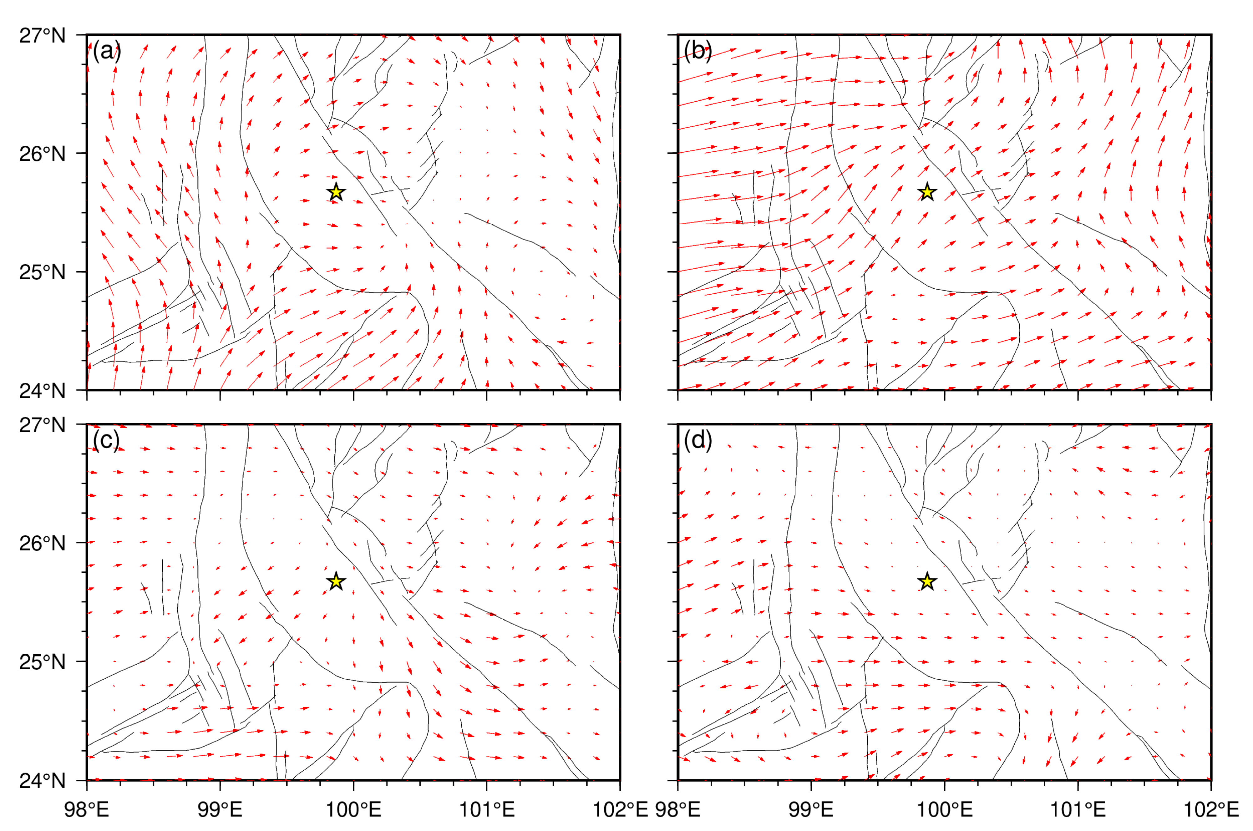
3.1. TSF Characteristics

Figure 2 and Table 2 display the inversion results of the TSF before the Ms 6.4 Yangbi earthquake. The compromise curve between the stress field inversion fitting error and the length of the model (or the complexity of the model) is shown in Figure 2a. The number marked on the right of the circle in the figure is the value of the damping coefficient, and the cross is the calculated optimal damping coefficient (inflection point). The best stress field inversion result can be obtained at the inflection point, that is, when the optimal damping coefficient is 1.2, as shown in Figure 2b. The azimuth of the maximum horizontal principal compressive stress rotates counterclockwise from west to east and rotates clockwise from north to south, which is consistent with the results of previous studies [33,44,45]. In the epicentral area (100° E, 26° N), the azimuths and plunges of the optimal solutions of σ1, σ2, and σ3 are −4.4° and 2.7°, −175.2°and 87.3°, 85.6°and 0.4°, respectively, and the corresponding 95% confidence intervals for azimuth of σ1, σ2, and σ3 are −183.1°~166.8°, −355.2°~4.3°, and 78.2°~91.5°, respectively.
The relative stress magnitude R is defined as [7]
R = σ 2 σ 1 σ 3 σ 1 .
The R value is the minimum at grid points (100° E, 27° N) and (101° E, 27° N), and the optimal solution is 0.07; the maximum is at (98° E, 25° N), and the optimal solution is 0.45; the optimal solution for the R value in the epicentral area (100° E, 26° N) is 0.13, and the 95% confidence interval is (0.00~0.30), as shown in Figure 2c.
We also inverted the TSF in the epicentral region of the Ms 6.4 Yangbi earthquake. The inversion parameters were the same as above, and the results are shown in Figure 2d. The optimal solution of the relative stress R value is 0.32. The azimuth of σ1 is 172.7° (150.8°~316.7°), and the plunge is 6.6° (−75.8°~88.3°). The azimuth of the minimum principal stress axis σ3 is 82.4° (73.6°~98.6°), and the plunge is 2.4° (−10.8°~15.0°).

3.2. Variations in Regional LGF

Figure 3a,d,g,j show the dynamic variation characteristics of D from 3 years before the earthquake to 1 month afterwards. The D near the epicenter continued to increase by 0.05′, as shown in Figure 3a,d. Before the earthquake (Figure 3g), D decreased slightly and then rebounded after the earthquake (Figure 3j). During this period, there were local anomalies with annual changes in D near the epicenter, and the epicenter was in the transition zone between two local anomalies. The positive anomaly areas are shown on the northern and southern sides and the negative anomaly areas on the eastern and western sides in Figure 3a; the large value areas of positive anomaly are present on the eastern and western sides of Figure 3d; the local isolated negative anomaly areas and their surrounding positive anomaly areas are illustrated in Figure 3g; and the positive anomaly areas on the southern side and negative anomalies on the northern side are shown in Figure 3j. Positive and negative anomalies coexisted in the area near the epicenter, and the epicenter was located near the “zero value” in annual D before (Figure 3g) and after (Figure 3j) the earthquake.
The dynamic changes in I are shown in Figure 3b,e,h,k. There are obvious abnormal areas at the epicenter, such as the positive anomaly on the northeastern side in Figure 3b, the large value areas of negative anomaly on the southwestern side in Figure 3e, the negative anomaly on the western side in Figure 3h, and the negative anomalies on the eastern and western sides in Figure 3k. Before (Figure 3h) and after the earthquake (Figure 3k), the epicenter was located near the “zero value” in annual I.
Figure 3c,f,i,l show the dynamic characteristics of F of the geomagnetic field. In Figure 3c, the negative anomaly area was located in the northeast of the epicenter, the positive anomaly area was located in the southwest, and the epicenter was located in the transition area from small to large of the positive anomaly area. The positive and negative anomalies areas in Figure 3f were opposite to those in Figure 3c. The northeast of the epicenter was a positive anomaly area, the southwest was a negative anomaly area, and the epicenter was located in the transition area from large to small of the negative anomaly. In subgraphs c and f, the areas of positive and negative anomalies were large and continuous. There was no obvious law of positive and negative anomalies in Figure 3i,l, the anomaly areas were relatively small and discontinuous, and the epicenter was located near the “zero value”.
According to the three components of D/I/F, we calculated the changes in the north component (X), east component (Y), horizontal component (H) and vertical component (Z) of the geomagnetic field. The annual changes in seven components of the geomagnetic field at different times within a radius of 50 km away from the epicenter of the Yangbi earthquake are reported, as shown in Table 3.

4. Discussion

4.1. Analysis of Geomagnetic Field Changes Based on the Meta-Instability Theory

Figure 4 gives the phase-by-phase variations in the horizontal vector of the LGF in the western Yunnan region before and after the Yangbi earthquake. The first three panels are all drawn based upon the observational data before the earthquake, while the last panel is the observational data before (one month) and after (one month) the earthquake.
Figure 4a shows the changes from 2018 to 2019. There are obvious low values in most areas from west to east of the Yongsheng-Binchuan fault and around the connection between the Weixi-Qiaohou-Weishan fault and the Honghe fault. The horizontal vector direction is divided into two different trends from west to east and from south to north at the intersection of the Longling-Lancang fault and the Wanding-Anding fault. With the direction of the trend distribution, the change in its value gradually decreases. When the fault is in the meta-instability stage after the peak stress intensity, it has entered an irreversible deformation stage, which indicates that the occurrence of earthquakes is inevitable [34]. According to the theory of meta-instability, there is a peak stress point around the Yongsheng-Binchuan fault zone before the meta-instability stage begins, and the magnitude in the surrounding area is relatively small. This indicates that the surrounding area is subjected to regional stress loading, which is a metastable state.
Figure 4b shows the variations from 2019 to 2020. The local area enclosed by the arc section of the Lancangjiang fault, the western branch of the Nanninghe fault, the Longling-Lancang fault and the Kejie fault is an area where the value of the horizontal vector is low. The horizontal vector direction is generally oriented from west to east from the Nujiang fault and Wanding-Anding fault and gradually becomes south to north after passing through the Honghe fault and Yongsheng-Binchuan fault. Compared with the vector in the previous period (2018 to 2019), the vector is roughly oriented in the same direction, but its magnitude is greater than that of the previous period. Compared with the change in Figure 4a, the “weakly variable area” migrates from northeast to southwest. According to the determination of the vector direction and magnitude, this area is still undergoing a stress loading process in the region, or it is in a metastable state.
Figure 4c shows the changes from 2020 to 2021. Compared with Figure 4b, the horizontal vector in the variation diagram in Figure 4c is generally small, and a “weak variation area” crosses the epicenter and appears on the northern and southern sides of the epicenter. Among them, the “weakly variable areas” on the northern side are distributed from west to east on the Weixi-Qiaohou-Weishan fault, Lancangjiang fault, and Nujiang fault. The magnitudes of local areas reach zero. In addition, the weak variation areas on the southern side are along the Lancangjiang fault and Kejie fault. The magnitude of the local area near the intersection also reaches zero. The horizontal vector directions spreading to the southeast and southwest from the epicenter show divergent trends from northwest to southeast and northeast to southwest, respectively, and the corresponding magnitudes also increase from small to large. The scope of the “weak variation area” is seen to have expanded compared with those of the previous two periods, and the northern and southern sides are around the epicenter. At the same time, the horizontal vector direction is completely reversed in the southwestern part of the Weixi-Qiaohou-Weishan fault compared with those of the previous two periods, and there is a clockwise rotation of nearly 90° in the vector direction around the Honghe fault. From the analysis of the above characteristics, a large-scale “weak variation region” appears in this period, accompanied by the change in vector direction and a gradual increase in magnitude in two local regions; these features indicate that the region with the change in vector direction has completely entered the metastable state, which implies that an earthquake will inevitably occur. The observation in western Yunnan was completed approximately 15 days before the earthquake, which shows that the observed anomalous characteristics of the metastable state occurred 15 days after the Yangbi MS 6.4 earthquake, and that its epicenter was located at the edge of the “weak variation area”.
Figure 4d shows the variation from May–June 2021. For the coseismic effect of the horizontal vector of the LGF associated with the Yangbi earthquake, the vector magnitude in the region from the Weixi-Qiaohou-Weishan fault to the Yongsheng-Binchuan fault reached a value of zero, which indicates that the stress loading in this area was still at the peak stage. From the Weixi-Qiaohou-Weishan fault to the west along the Lancangjiang fault and then to the Nujiang fault, the vector direction spread from west to east, and the magnitude gradually increased. There are two situations in this area: stress remains loaded, or strain is released. These results also show that the seismomagnetic effect does not subside rapidly in a short time after the earthquake.
The results of the TSF show that the azimuth of σ1 in the epicentral area was NNW, close to positive N, before the Yangbi earthquake, and changed to SSE, close to the positive S direction, after the earthquake [33]. The seismogenic structure is subjected to dextral strike-slip movement under the regional stress of near north-south compression and east-west tension. The formation of the structure may be associated with the SE slip of the Sichuan-Yunnan block and the clockwise rotation of the Southwest Yunnan block [35].

4.2. Seismomagnetic Mechanism

The performance and mechanisms of geomagnetic anomalies in the early stages of earthquakes are very complex, involving geomagnetic anomalies generated by the continuous changes of the source, regional stress fields, and other factors related to earthquakes [16,26,27]. It is necessary to separate earthquake-related anomalous signals from the collected geomagnetic anomaly signals, as these signals may be caused by earthquakes and other factors. Additionally, these measured geomagnetic signals mainly include the basic magnetic field and the changing magnetic field; the abnormal changes of the geomagnetism are also affected by these two parts. Therefore, it is necessary to filter out the geomagnetic anomaly caused by the changing magnetic field unrelated to the earthquake. Diurnal and secular variation corrections are made in observational data precisely to ensure the acquisition of reliable geomagnetic anomalies.
Tectonic activities such as earthquakes and volcanoes are very complex physical processes, often accompanied by subsurface thermal convection, causing changes in temperature, pressure, and fluid movement. The physical mechanisms leading to the magnetic anomalies caused by these tectonic activities are not unique. Besides the piezomagnetic effect related to the change of rock magnetization caused by stress, they also include the electrokinetic effect caused by the existence of electric double layer at the solid-liquid interface, the thermal demagnetization effect caused by temperature, etc. [15,20]. Song et al. calculated the piezomagnetic and electrokinetic effects probably produced by the Yangbi earthquake, and found that the changes at a distance of 20 km from the epicenter were −0.3 nT and −0.2 nT, respectively, which were much smaller than the actually observed change in the geomagnetic field [46]. Therefore, a single mechanism cannot effectively explain the geomagnetic field changes before and after the Yangbi earthquake, and it is necessary to synthesize a variety of data for quantitative analysis.

5. Conclusions

The TSFs near the epicenter before and after the Yangbi earthquake were inverted by using the FMS around the epicenter. Based on repeated observational data for 27 ground geomagnetic survey vectors within 250 km of the Yangbi earthquake epicenter, an annual variation model of the geomagnetic field around the epicenter from 3 years before the earthquake to 1 month afterwards was constructed. Based on the laboratory meta-instability theoretical model, the annual variation model of the horizontal vector of the geomagnetic field was used to analyze the buildup, occurrence and evolution of the Yangbi earthquake. We reached the following important conclusions:
(1)
The azimuth of the maximum principal compressive stress axis of the TSF in the epicentral area was deflected nearly 180 degrees from before to after the Yangbi earthquake.
(2)
The epicenter was not located in the area with large values of annual anomalous variations in the geomagnetic field but near the area with zero variation and its adjacent area.
(3)
The area was found to have entered the meta-instability stage one year before the earthquake.
In the meta-instability stage, the fault is in an irreversible deformation stage, which indicates that an earthquake will inevitably occur. However, the application of meta-instability research from the laboratory to the field is an extension from one-dimensional linear results to a two-dimensional plane. The phase-by-phase variation distribution of the horizontal vector of the geomagnetic field shows that the above four states coexist in the same region, and these four states can be transformed with time in a spatial region. During this transformation, the boundary zone of the “weak variation region” of the horizontal vector is the potential epicentral region and is the most easily recognized sign in the field before the area enters the meta-instability stage. The spatiotemporal evolution of the “weakly variable region” and the change in the surrounding vector direction are the basic conditions for analyzing whether the epicentral region will enter the meta-instability stage in the future.
The results are of great value for the study of the earthquake incubation environment and the source of local geomagnetic anomalies, and play a theoretical guiding role in the identification of magnetic field anomalies that are precursors to earthquakes.
This paper does not present a more in-depth analysis of the corresponding (or quantitative) relationship between the TSF and LGF before and after the earthquake, as this will be covered in future research.

Author Contributions

Data curation, S.C. and S.S.; Formal analysis, Z.W., Z.N. and S.S.; Funding acquisition, J.Y.; Investigation, Z.N. and S.C.; Methodology, Z.W. and Z.N.; Project administration, J.Y.; Resources, Z.W.; Software, Z.W.; Supervision, Z.N.; Validation, S.S. and J.Y.; Visualization, S.C.; Writing—original draft, Z.W. All authors have read and agreed to the published version of the manuscript.

Funding

This research was funded by the National Key Research and Development Program of China, grant number 2018YFC150330504.

Institutional Review Board Statement

Not applicable.

Informed Consent Statement

Not applicable.

Data Availability Statement

The data presented in this study are available on request from the corresponding author.

Acknowledgments

The authors used Generic Mapping Tools to make many of the figures in this article [47]. We thank the Geomagnetic Network of China for providing the geomagnetic field data for this study. We also thank the Harvard University for providing the Global CMT Catalog (http://www.globalcmt.org/ (accessed on 16 January 2022)).

Conflicts of Interest

The authors declare no conflict of interest.

References

  1. Mao, Z.; Chen, C.H.; Zhang, S.; Yisimayili, A.; Yu, H.; Yu, C.; Liu, J.Y. Locating Seismo-Conductivity Anomaly before the 2017 Mw 6.5 Jiuzhaigou Earthquake in China Using Far Magnetic Stations. Remote Sens. 2020, 12, 1777. [Google Scholar] [CrossRef]
  2. Sarlis, N.V. Statistical Significance of Earth’s Electric and Magnetic Field Variations Preceding Earthquakes in Greece and Japan Revisited. Entropy 2018, 20, 561. [Google Scholar] [CrossRef] [Green Version]
  3. Sasmal, S.; Chowdhury, S.; Kundu, S.; Politis, D.Z.; Potirakis, S.M.; Balasis, G.; Hayakawa, M.; Chakrabarti, S.K. Pre-Seismic Irregularities during the 2020 Samos (Greece) Earthquake (M = 6.9) as Investigated from Multi-Parameter Approach by Ground and Space-Based Techniques. Atmosphere 2021, 12, 1059. [Google Scholar] [CrossRef]
  4. Wang, Z.; Yuan, J.; Chen, B.; Chen, S.; Wang, C.; Mao, F. Local magnetic field changes during gas injection and extraction in an underground gas storage. Geophys. J. Int. 2019, 217, 271–279. [Google Scholar] [CrossRef]
  5. Lin, J.; Stein, R.S. Stress triggering in thrust and subduction earthquakes and stress interaction between the southern San Andreas and nearby thrust and strike-slip faults. J. Geophys. Res. Solid Earth 2004, 109, B02303. [Google Scholar] [CrossRef] [Green Version]
  6. Ellsworth, W.L.; Xu, Z.H. Determination of the stress tensor from focal mechanism data. EOS Trans. Am. Geophys. Union 1980, 61, 1117. [Google Scholar]
  7. Gephart, J.W.; Forsyth, D.W. An improved method for determining the regional stress tensor using earthquake focal mechanism data: Application to the San Fernando earthquake sequence. J. Geophys. Res. Solid Earth 1984, 89, 9305–9320. [Google Scholar] [CrossRef]
  8. Lund, B.; Townend, J. Calculating horizontal stress orientations with full or partial knowledge of the tectonic stress tensor. Geophys. J. Int. 2007, 170, 1328–1335. [Google Scholar] [CrossRef] [Green Version]
  9. Michael, A.J. Use of focal mechanisms to determine stress: A control study. J. Geophys. Res. 1987, 92, 357–368. [Google Scholar] [CrossRef]
  10. Sun, Y.; Zhao, X.; Huang, Y.; Yang, H.; Li, F. Characteristic of focal mechanisms and stress field of Yunnan area. Seismol. Geol. 2017, 39, 390–407. (In Chinese) [Google Scholar]
  11. Blakely, R.J. Geomagnetism and Paleomagnetism. Rev. Geophys. 1987, 25, 895–899. [Google Scholar] [CrossRef]
  12. Witze, A. Earth’s magnetic field is acting up and geologists don’t know why. Nature 2019, 565, 143–144. [Google Scholar] [CrossRef]
  13. Qiu, Y.; Wang, Z.; Jiang, W.; Zhang, B.; Li, F.; Guo, F. Combining CHAMP and Swarm Satellite Data to Invert the Lithospheric Magnetic Field in the Tibetan Plateau. Sensors 2017, 17, 238. [Google Scholar] [CrossRef] [Green Version]
  14. Thébault, E.; Purucker, M.; Whaler, K.A.; Langlais, B.; Sabaka, T.J. The Magnetic Field of the Earth’s Lithosphere. Space Sci. Rev. 2010, 155, 95–127. [Google Scholar] [CrossRef]
  15. Gao, Y.; Harris, J.M.; Wen, J.; Huang, Y.; Twardzik, C.; Chen, X.; Hu, H. Modeling of the coseismic electromagnetic fields observed during the 2004 Mw 6.0 Parkfield earthquake. Geophys. Res. Lett. 2016, 43, 620–627. [Google Scholar] [CrossRef] [Green Version]
  16. Liu, X.; Hattori, K.; Han, P.; Chen, H.; Chie, Y.; Zhao, X. Possible anomalous changes in solar quiet daily geomagnetic variation (Sq) related to the 2011 off the Pacific coast of Tohoku Earthquake (Mw 9.0). Pure Appl. Geophys. 2020, 177, 333–346. [Google Scholar] [CrossRef]
  17. Marchetti, D.; De Santis, A.; Campuzano, S.A.; Soldani, M.; Piscini, A.; Sabbagh, D.; Cianchini, G.; Perrone, L.; Orlando, M. Swarm Satellite Magnetic Field Data Analysis Prior to 2019 Mw = 7.1 Ridgecrest (California, USA) Earthquake. Geosciences 2020, 10, 502. [Google Scholar] [CrossRef]
  18. Johnston, M.J.S. Review of magnetic and electric field effects near active faults and volcanoes in the USA. Phys. Earth Planet. Inter. 1989, 57, 47–63. [Google Scholar] [CrossRef]
  19. McGarr, A.; Zoback, M.D.; Hanks, T.C. Implications of an elastic analysis of in situ stress measurements near the San Andreas fault. J. Geophys. Res. 1982, 87, 7797–7806. [Google Scholar] [CrossRef] [Green Version]
  20. Hao, J.; Hastie, L.M.; Stacey, F.D. Theory of the seismomagnetic effect a reassessment. Phys. Earth Planet. Inter. 1982, 28, 129–140. [Google Scholar] [CrossRef]
  21. Florio, G.; Fedi, M.; Rapolla, A.; Fountain, D.M.; Shive, P.N. Anisotropic magnetic susceptibility in the continental lower crust and its implications for the shape of magnetic anomalies. Geophys. Res. Lett. 1993, 20, 2623–2626. [Google Scholar] [CrossRef]
  22. Gorev, R.V.; Udalov, O.G. Micromagnetic simulation of the magnetoelastic effect in submicron structures. Phys. Solid State 2019, 61, 1563–1571. [Google Scholar] [CrossRef]
  23. Breiner, S. Piezomagnetic effect at the time of local earthquakes. Nature 1964, 202, 790–791. [Google Scholar] [CrossRef]
  24. Roskosz, M.; Rusin, A.; Bieniek, M. Analysis of relationships between residual magnetic field and residual stress. Meccanica 2013, 48, 45–55. [Google Scholar] [CrossRef] [Green Version]
  25. Wang, Z.; Chen, B.; Yuan, J.; Yang, F.; Jia, L.; Wang, C. Localized geomagnetic field anomalies in an underground gas storage. Phys. Earth Planet. Inter. 2018, 283, 92–97. [Google Scholar] [CrossRef]
  26. Chen, C.H.; Liu, J.Y.; Lin, P.Y.; Yen, H.Y.; Hattori, K.; Liang, W.T.; Chen, Y.I.; Yeh, Y.H.; Zeng, X. Pre-seismic geomagnetic anomaly and earthquake location. Tectonophysics 2010, 489, 240–247. [Google Scholar] [CrossRef]
  27. Han, P.; Zhuang, J.; Hattori, K.; Chen, C.-H.; Febriani, F.; Chen, H.; Yoshino, C.; Yoshida, S. Assessing the Potential Earthquake Precursory Information in ULF Magnetic Data Recorded in Kanto, Japan during 2000–2010: Distance and Magnitude Dependences. Entropy 2020, 22, 859. [Google Scholar] [CrossRef] [PubMed]
  28. Gilder, S.A.; LeGoff, M.; Peyronneau, J.; Chervin, J.C. Novel high pressure magnetic measurements with applications to magnetite. Geophys. Res. Lett. 2002, 29, 1392. [Google Scholar] [CrossRef] [Green Version]
  29. Nagata, T. Anisotropic magnetic susceptibility of rocks under mechanical stresses. Pure Appl. Geophys. 1970, 78, 110–122. [Google Scholar] [CrossRef]
  30. Stacey, F.D.; Johnston, M.J.S. Theory of the piezomagnetic effect in titanomagnetite-bearing. Pure Appl. Geophys. 1972, 97, 146–155. [Google Scholar] [CrossRef] [Green Version]
  31. Yamazaki, K. Temporal variations in magnetic signals generated by the piezomagnetic effect for dislocation sources in a uniform medium. Geophys. J. Int. 2016, 206, 130–141. [Google Scholar] [CrossRef]
  32. Zhan, Z. Investigations of tectonomagnetic phenomena in China. Phys. Earth Planet. Inter. 1989, 57, 11–22. [Google Scholar]
  33. Lei, X.L.; Wang, Z.W.; Ma, S.L.; He, C.R. A preliminary study on the characteristics and mechanism of the May 2021 MS6.4 Yangbi earthquake sequence, Yunnan, China. Acta Seismol. Sin. 2021, 43, 261–286. (In Chinese) [Google Scholar]
  34. Ma, J. On “whether earthquake precursors help for prediction do exist”. Chin. Sci. Bull. 2016, 61, 409–414. (In Chinese) [Google Scholar] [CrossRef] [Green Version]
  35. Long, F.; Qi, Y.; Yi, G.; Wu, W.; Wang, G.; Zhao, X.; Peng, G. Relocation of the Ms 6.4 Yangbi earthquake sequence on May 21, 2021 in Yunnan Province and its seismogenic structure analysis. Chin. J. Geophys. 2021, 64, 2631–2646. (In Chinese) [Google Scholar]
  36. Deng, Q.D.; Zhang, P.Z.; Ran, Y.K.; Yang, X.P.; Min, W.; Chen, L.C. Active tectonics and earthquake activities in China. Earth Sci. Front. 2003, 10, 66–73. (In Chinese) [Google Scholar]
  37. Dziewonski, A.M.; Chou, T.A.; Woodhouse, J.H. Determination of earthquake source parameters from waveform data for studies of global and regional seismicity. J. Geophys. Res. 1981, 86, 2825–2852. [Google Scholar] [CrossRef]
  38. Ekström, G.; Nettles, M.; Dziewonski, A.M. The global CMT project 2004-2010: Centroid-moment tensors for 13,017 earthquakes. Phys. Earth Planet. Inter. 2012, 200–201, 1–9. [Google Scholar] [CrossRef]
  39. Gu, Z.; Zhan, Z.; Gao, J.; Han, W.; An, Z.; Yao, T.; Chen, B. Geomagnetic survey and geomagnetic model research in China. Earth Planets Space 2006, 58, 741–750. [Google Scholar] [CrossRef] [Green Version]
  40. Menke, W. Nonlinear Inverse Problems. In Geophysical Data Analysis: Discrete Inverse Theory, 3rd ed.; Academic Press: San Diego, CA, USA, 2012; pp. 163–188. [Google Scholar]
  41. Hardebeck, J.L.; Michael, A.J. Damped regional-scale stress inversions: Methodology and examples for southern California and the Coalinga aftershock sequence. J. Geophys. Res. Solid Earth 2006, 111, B11310. [Google Scholar] [CrossRef]
  42. Martínez-Garzón, P.; Kwiatek, G.; Ickrath, M.; Bohnhoff, M. MSATSI: A MATLAB© package for stress inversion combining solid classic methodology, a new simplified user-handling and a visualization tool. Seismol. Res. Lett. 2014, 85, 896–904. [Google Scholar] [CrossRef] [Green Version]
  43. Gao, Q.; Cheng, D.; Wang, Y.; Li, S.; Wang, M.; Yue, L.; Zhao, J. Compensation method for diurnal variation in three-component magnetic survey. Appl. Sci. 2020, 10, 986. [Google Scholar] [CrossRef] [Green Version]
  44. Wang, M.; Shen, Z.K. Present-day crustal deformation of continental China derived from GPS and its tectonic implications. J. Geophys. Res. Solid Earth 2020, 125, e2019JB018774. [Google Scholar] [CrossRef] [Green Version]
  45. Xu, Y.; Koper, K.D.; Burlacu, R.; Herrmann, R.B.; Li, D.N. A New Uniform Moment Tensor Catalog for Yunnan, China, from January 2000 through December 2014. Seismol. Res. Lett. 2020, 91, 891–900. [Google Scholar] [CrossRef]
  46. Song, C.; Chen, Z.; Zhou, S.; Xu, Y.; Chen, B. Geomagnetic field change before and after 2021 Yangbi Ms 6.4 earthquake. Seismol. Geol. 2021, 43, 958–971. (In Chinese) [Google Scholar] [CrossRef]
  47. Wessel, P.; Luis, J.F.; Uieda, L.; Scharroo, R.; Wobbe, F.; Smith, W.H.F.; Tian, D. The Generic Mapping Tools version 6. Geochem. Geophys. Geosyst. 2019, 20, 5556–5564. [Google Scholar] [CrossRef] [Green Version]
Figure 1. The epicenter of the Yangbi Ms 6.4 earthquake and the research area. The yellow pentagram is the epicenter of the MS 6.4 mainshock, the black solid lines show the distribution of faults [36], the blue triangles represent the distribution of repeat measurement stations of the magnetic field vector, and the red triangles represent the continuously recording geomagnetic observatories.
Applsci 12 01005 g001
Figure 2. Results of stress field inversion. (a) Tradeoff between the length of the model and data misfit for different values of the damping parameters. The damping values are shown next to each point. The final selected damping parameter is represented by a cross. (b) Spatial distribution of the stress field orientation. The axes of the maximum compressive stress, intermediate principal stress and minimum compressive stress are represented as σ1, σ2, and σ3, respectively. The 95% confidence limits of σ1, σ2, and σ3 are marked with red, green and blue points, respectively. The best solutions are indicated by black crosses. (c) Confidence limits of the R value corresponding to (b). (d) Stress field direction and R value of the Yangbi earthquake using 13 FMSs.
Applsci 12 01005 g002
Figure 3. Contour map of the annual variations in the D/I/F components of the LGF in the epicentral and surrounding areas of the Yangbi earthquake. The three figures (ac) in the first row are the annual changes from May 2018 to May 2019, the second row (df) shows the annual changes from May 2019 to May 2020, the third row (gi) illustrates the changes from May 2020 to May 2021, and the fourth row (jl) shows the changes from May–June 2021. The four pictures in the first column are the D component (unit is ′), those in the second column are the I component (unit is ′), and those in the third column are the F component (unit is nT).
Applsci 12 01005 g003
Figure 4. Annual variations in the horizontal vector of the magnetic field in the epicentral and surrounding areas of the Yangbi earthquake. (a) The annual change from May 2018 to May 2019, (b) the change from May 2019 to May 2020, (c) the change from May 2020 to May 2021, and (d) the change from May–June 2021. The direction of the arrow represents the horizontal vector direction, and the size of the arrow is 1° = 50 nT.
Applsci 12 01005 g004
Table 1. FMSs of the typical Ms > 4.0 event of the Yangbi earthquake sequence.
Earthquake TimeEpicenter LocationMagnitudeFault-Plane IFault-Plane II
Longitude (°)Latitude (°)MsStrikeDipRakeStrikeDipRake
2021.5.18 21:3999.9325.654.24178830982168
2021.5.19 20:0599.9125.654.422990−1531975180
2021.5.21 20:5699.9325.644.215945−1151250−67
2021.5.21 21:2199.9325.655.621786−1230878−176
2021.5.21 21:4899.8825.696.413575−1684278−15
2021.5.21 21:5699.9525.644.9220842012870174
2021.5.21 22.1599.9725.604.0128801602227011
2021.5.21 22.2199.9825.605.214648−1614376−44
2021.5.21 23:2399.9825.604.512787177217873
2021.5.22 00:5199. 8725.694.03585−912681−175
2021.5.22 09:4899.8825.674.031384−17622386−6
2021.5.22 20:1499.9325.614.432544−14020463−54
2021.5.27 19:5299.9525.744.119490−528485180
Table 2. Results of stress field.
Locationσ1σ2σ3R Value
AzimuthPlungeAzimuthPlungeAzimuthPlungeR BestR MinR Max
(98° E, 25° N)−159.210.356.277.4−67.97.10.450.000.72
(99° E, 24° N)−169.74.221.285.7−79.60.80.350.010.67
(99° E, 25° N)−170.24.921.785.0−80.11.00.340.010.69
(99° E, 26° N)−177.11.3−8.788.792.90.30.220.000.35
(100° E, 25° N)1.02.5169.087.4−89.10.50.210.010.38
(100° E, 26° N)−4.42.7−175.287.385.60.40.130.000.30
(100° E, 27° N)−8.021.7174.168.382.30.70.070.000.23
(101° E, 25° N)174.31.445.687.7−95.71.80.210.000.42
(101° E, 26° N)170.56.2−16.883.780.40.80.240.010.49
(101° E, 27° N)−11.224.0176.265.880.02.80.070.010.27
(102° E, 26° N)−10.61.7−128.586.479.53.10.310.010.53
Table 3. The magnitude of the annual variation in each component of the magnetic field at the epicenter of the Yangbi earthquake and within a radius of 50 km. The upper row corresponding to each component is the amplitude of the epicenter position, and the lower row is the variation amplitude within a radius of 50 km around the epicenter.
ComponentsDifferent Annual Variation Cycles
May 2018 to May 2019May 2019 to May 2020May 2020 to May 2021May–June 2021
Declination
(′)
0.860.91−0.200.07
0.18~0.960.65~1.31−0.67~0.51−0.37~0.78
Inclination
(′)
0.54−1.730.29−0.12
−0.25~0.65−2.43~−1.03−0.26~0.67−0.18~0.27
Total intensity
(nT)
3.8−7.3−1.7−1.9
1.9~5.0−11.2~−4.7−7.6~1.1−3.0~1.5
North component
(nT)
−1.710.1−3.9−0.4
−2.4~4.74.3~14.2−5.8~−1.2−1.4~1.7
East component
(nT)
9.29.6−2.00.7
1.9~10.16.9~13.8−7.1~5.6−4.0~8.5
Horizontal intensity
(nT)
−1.99.9−3.8−0.4
−2.6~4.74.1~14.0−6.5~−0.5−1.5~1.8
Vertical intensity
(nT)
8.3−23.22.0−2.5
−1.4~9.6−15.5~−33.1−7.9~7.0−3.9~3.6
Publisher’s Note: MDPI stays neutral with regard to jurisdictional claims in published maps and institutional affiliations.

