Smartphone-Based Photogrammetry Assessment in Comparison with a Compact Camera for Construction Management Applications

Featured Application

This study aimed towards making close-range photogrammetry more accessible and affordable for on-site construction management applications that involve data modeling and measurements extractions by utilizing smartphones directly without a pre-calibration procedure. This article is expected to provide a thorough assessment of the quality and geometrical accuracy of smartphones’ photogrammetric results compared with a digital compact camera. This work is a part of ongoing research on adapting photogrammetry as a tracking and forecasting technique for earthmoving operations in heavy construction projects.

Abstract

Close-range photogrammetry (CRP) has proven to be a remarkable and affordable technique for data modeling and measurements extraction in construction management applications. Nevertheless, it is important to aim for making CRP more accessible by using smartphones on-site directly without a pre-calibration procedure. This study evaluated the potential of smartphones as data acquisition tools in comparison with compact cameras based on the quality and accuracy of their photogrammetric results in extracting geometrical measurements (i.e., surface area and volume). Two concrete specimens of regular shapes (i.e., beam and cylinder) along with an irregular-shaped sand pile were used to conduct this study. The datasets of both cameras were analyzed and compared based on lens distortions, image residuals, and projections multiplicity. Furthermore, the photogrammetric models were compared according to various quality criteria, processing time, and memory utilization. Though both cameras were not pre-calibrated, they both provided highly accurate geometrical estimations. The volumetric estimation error ranged from 0.37% to 2.33% for the compact camera and 0.67% to 3.19% for the smartphone. For surface area estimations, the error ranged from 0.44% to 0.91% for the compact camera and 0.50% to 1.89% for the smartphone. Additionally, the smartphone data required less processing time and memory usage with higher applicability compared with the compact camera. The implication of these findings is that they provide professionals in construction management with an assessment of a more direct and cost-effective 3D data acquisition tool with a good understanding of its reliability. Moreover, the assessment methodology and comparison criteria presented in this study can assist future research in conducting similar studies for different capturing devices in construction management applications. The findings of this study are limited to small quantification applications. Therefore, it is recommended to conduct further research that assesses smartphones as a photogrammetric data acquisition tool for larger construction elements or tracking ongoing construction activities that involve measurements estimation.

1. Introduction

The ability to provide accurate geometrical estimations (e.g., surface areas and materials volumes) is essential in the field of construction management since they are a key for generating accurate quantity take-off and cost estimation reports during tasks planning. They are also essential for progress tracking and forecasting during tasks’ implementation. Additionally, accurate progress measurements can be used as input data for simulating and optimizing construction tasks. For instance, a crew working on an earthmoving operation can be optimized based on its measured actual performance, thus resulting in an optimum crew configuration with the least cost [1]. In most construction projects, conventional methods of estimation, which are time-consuming, cost-ineffective, and error-prone, continue to be used. On the other hand, the technology of digital photogrammetry, both terrestrial and aerial, was established to be a remarkable data collection approach for 3D data modeling and measurements extraction in various construction applications, such as building modeling and documentation [2,3,4], progress tracking [5,6,7,8,9], and measurement extractions [10,11]. Although most of the research integrating photogrammetry with construction management is focused mainly on assessing and utilizing the aerial type using UAV platforms due to their higher efficiency to cover large areas [2,6,11], close-range photogrammetry can be suitable for scanning relatively smaller areas and tracking indoor tasks.

Close range photogrammetry (CRP) processes ground-based overlapping images via a structure from motion (SFM) pipeline. The processing starts by implementing the scale invariant feature transform (SIFT) algorithm [12,13,14] or similar algorithms (e.g., SURF and ORB). SIFT detects images’ features and matches those shared by overlapping images by comparing their descriptors. Through bundle block adjustment (BBA) [15,16,17,18], the camera calibration parameters (i.e., translating, rotation, focal lengths, the optical center, and lens distortions) are estimated and optimized. After estimating the camera poses, the matched features get reconstructed as 3D points by triangulating them from all overlapping images, resulting in a sparse point cloud. The sparse cloud can be densified by generating and merging depth maps of the overlapping images [19,20,21]. From the densified cloud, a polygonal mesh can be generated using mesh triangulation algorithms (e.g., Poisson reconstruction). For providing the polygonal mesh with a photorealistic appearance, a colored texture map is generated.

The accuracy and quality of these photogrammetric outputs depend significantly on the specification of the camera used for acquiring images. In most research, advanced compact cameras with high resolution and less distortion are used. Others used pre-calibrated cameras for which their calibration parameters were precisely determined before data capturing. For instance, one study [22] evaluated the accuracy of CRP as a measuring tool using a pre-calibrated digital compact camera. Nevertheless, it is important to aim for making CRP more accessible and feasible not only by utilizing inexpensive compact cameras but also by using smartphones directly without a pre-calibration procedure.

Nowadays, smartphones are associated with cameras that are of sufficient potential to provide reasonably high-quality images. Smartphones are highly accessible compared with compact cameras and can be utilized for acquiring photogrammetric images by any worker on a construction site. Additionally, smartphones excel compact cameras in their ability to send the collected images on-site to any processing device via Wi-Fi or Bluetooth, thus providing near real-time measurements. Therefore, it is essential to present a study that fully assesses the quality and accuracy of the 3D models generated from smartphone data and compares their results with those of a compact camera.

Most of the studies that evaluated CRP generally assessed its accuracy in extracting geometrical measurements. For instance, in the area of forestry, several studies [23,24,25,26] evaluated the accuracy of CRP in estimating tree attributes (e.g., tree radius, circumference, and height) extracted from point clouds generated from digital compact camera images. Similarly, in the area of engineering, some studies assessed CRP according to its accuracy in estimating models’ volumes [22,27,28] and deformation monitoring [29,30,31]. Other studies [32,33,34] in the area of cultural heritage evaluated CRP based on its quality for modeling and documenting architectural and archaeological structures.

Only a few studies aimed to investigate smartphone’s photogrammetric accuracy in general. For example, one study [27] evaluated CRP in estimating ground pile volume based on video frames captured by a digital camera and a smartphone. Their accuracy comparison was based only on the volumetric error. Another study [35] evaluated smartphones based on their potential and accuracy in modeling geomorphological structures. Another study [36] investigated the geometric accuracy of pre-calibrated smartphones’ cameras for which their internal parameters were determined. Even though pre-calibrated cameras in general result in more accurate results, calibrating a digital compact camera or a smartphone is a time-consuming step that requires a precise procedure and needs to be conducted for each camera intended to be used.

This study evaluated the potential of smartphones as an on-site data collection tool for data modeling and geometrical measurements extraction in comparison with a digital compact camera. The photogrammetric outputs (i.e., sparse cloud, dense cloud, polygonal, and textured models) of both cameras were compared based on their resulting parameters, processing time, and memory usage. Additionally, they were assessed and compared based on various quality criteria (e.g., sparse cloud noise, cloud density, points color, and texture representation). The accuracy of the 3D reconstruction for both data sets was examined based on the distortion parameters, RMS reprojection errors (i.e., image residuals), projections percentage, and tie multiplicity of the reconstructed points. These assessment criteria were selected based on previous studies [33,37,38,39] assessing digital photogrammetry and according to some photogrammetric software guides [40,41] in which various quality criteria and processing parameters were identified to impact the overall quality and reliability of the 3D reconstruction process and the different resulting outputs (e.g., tie points, dense clouds, and textured models). The study relied on the self-calibration approach conducted within the bundle adjustment algorithm based on the provided Exif data. Therefore, both cameras were not pre-calibrated, aiming to eliminate the camera calibration procedure required before capturing images; thus, any digital camera or smartphone can be utilized directly. Finally, both cameras were compared according to the estimation accuracy of the geometrical measurements (i.e., surface area and volume) extracted from the final textured 3D models of their data sets.

2. Materials and Methods

In this study, an average digital compact camera (Nikon-D 3300) and a smartphone (Huawei Mate 10 lite) were utilized to capture the photogrammetric data, Figure 1. The specifications of both cameras are provided in

Table 1. The specifications of the utilized cameras.

Specification	Digital Camera (Nikon-D 3300)	Smartphone (Huawei Mate 10 Lite)
Camera Model	D-3300	RNE-L21
Sensor Type	CMOS	BSI-CMOS
Sensor Size	APS-C (23.5 mm × 15.6 mm)	~1/2.9″ 4.8 × 3.6 mm
Camera Resolution	24 MP 6000 × 4000 (3:2)	Dual 16 MP + 2 MP 4608 × 3456 (4:3)
Pixel Size	4.04 μm	~1.06 μm
Focal Length (35 mm equivalent)	18–55 mm	27 mm
Crop Factor	1.43	6.75
Native ISO	100–12,800	50–3200
Aperture	f/3.5–f/5.6	f/1.6–f/2.2
Image Format	RAW (NEF), JPEG	JPG

.

It was important to start the assessment on construction elements with regular geometric shapes for which their volumes and surface areas can be easily measured so that measurement errors are eliminated, thus providing an accurate assessment. For this purpose, two specimens of casted concrete were made using standard molds of different shapes and sizes, i.e., a square beam (15.2 cm × 15.2 cm × 75.6 cm) and a cylinder (15 cm × 30 cm), Figure 2. In addition, a small sand pile (5490 cm³, Figure 2c) was formed to further assess the geometrical accuracy for irregular material.

Figure 3 presents the workflow followed by this study to assess and compare the quality of the photogrammetric outputs along with the geometrical accuracy of the final 3D models for both cameras’ data sets.

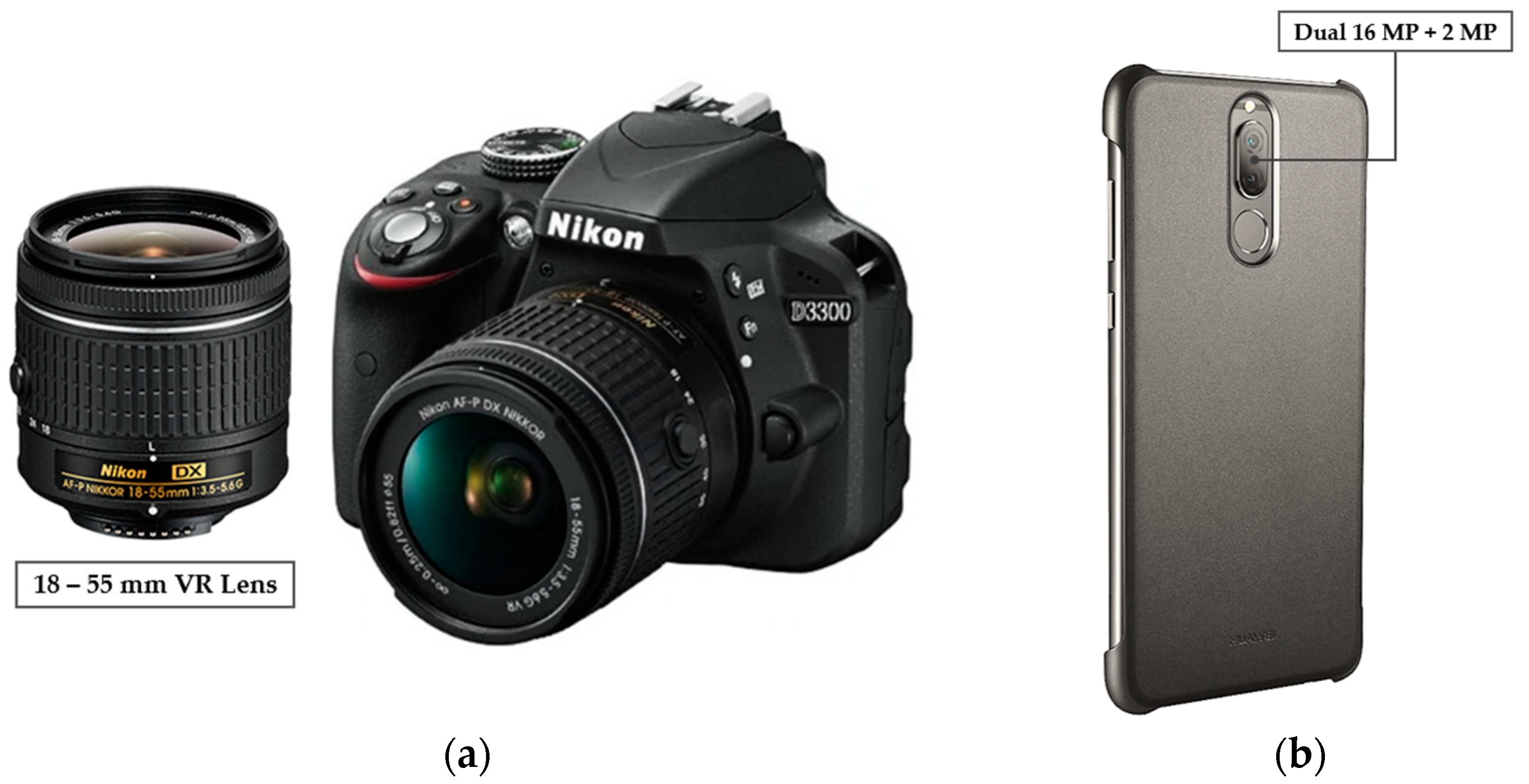
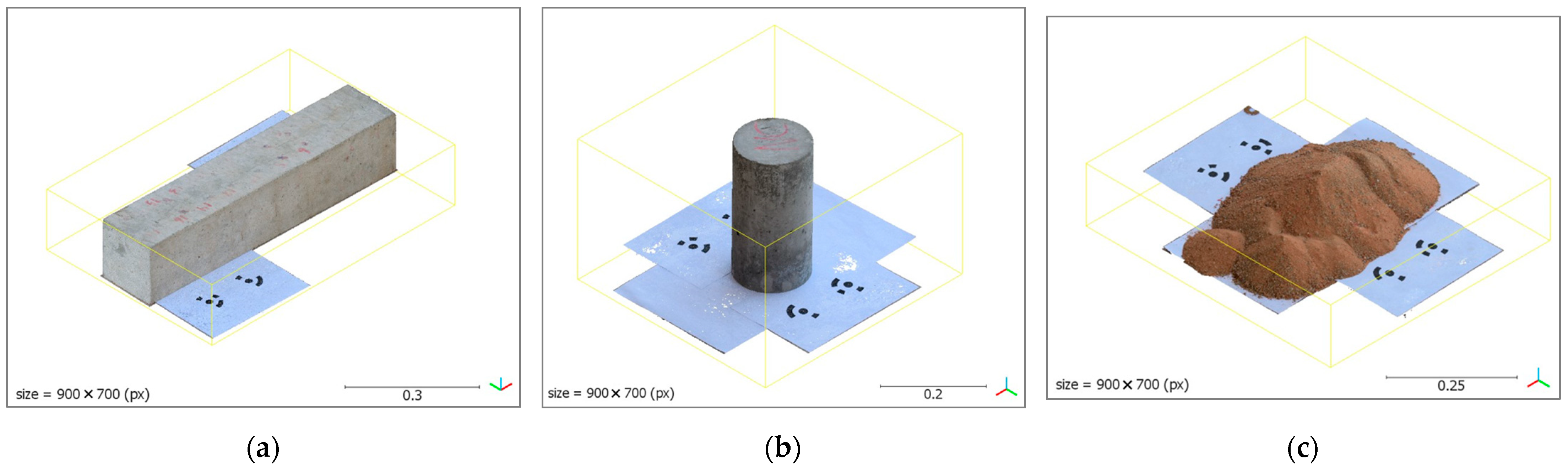
2.1. Data Acquisition

Before capturing images, a number of coded targets, at least two, had to be placed near the object of interest to be utilized as ground control points for scaling the generated 3D data. In this study, four coded targets were placed around each specimen.

Table 2. The capturing scenario parameters.

Specimen	Capturing Device	Number of Images	Image Quality	Covered Area (m2)
Square Beam	DC 1	43	0.842	0.337
	SP 2		0.894	0.474
Cylinder	DC	24	0.835	0.409
	SP		0.886	0.546
Sand Pile	DC	40	0.862	0.442
	SP		0.893	0.504

¹ Digital compact camera. ² Smartphone camera.

provides the number of images captured for each specimen. The same number of images was taken by both cameras for each specimen. Additionally, the images of each specimen were taken almost from the same positions, following the same track for both cameras. By doing so, the number of images, overlapping percentage, and camera movement were held the same for both cameras so that the accuracy and quality assessments would be entirely based on the camera specifications. The camera settings with which the images were captured are provided for both cameras in

Table 3. The cameras’ parameters with which the study images were captured.

Capturing Parameters	Digital Camera (Nikon-D 3300)	Smartphone (Huawei Mate 10 Lite)
Focal Length (35 mm equivalent)	35 (50)	4 (27)
ISO	400	50
F-stop	f/8	f/2.2
Shutter Speed	1/250	1/215
Image Format	RAW (NEF): TIFF-16bit	JPG

.

The image quality values provided in Table 2 present the average quality value ranging from 0 to 1 of all captured images in the same data set. This value was computed using a built-in function in Agisoft Metashape software [42]. It estimates the overall quality of a given image based on its level of sharpness relative to the other images in the same data set. It was shown that the average image quality of the smartphone images (SP) was slightly higher than those of the digital camera (DC). This was due to the image format; the compact camera images were taken with RAW (NEF) format, which prevents any auto adjustment to the image in terms of its brightness and sharpness. However, with the JPG format, the images’ level of brightness and sharpness were optimized automatically by a built-in feature in the smartphone camera (i.e., autofocus). Images with quality values less than 0.5 are recommended by Agisoft Metashape to be eliminated. In this study, all the images captured by both cameras had quality values greater than 0.7. Table 3 also shows that the area scanned with the smartphone camera was greater relative to the digital camera for all specimens. This is attributed mainly to the camera focal length. The shorter the focal length, the wider the angle of view, and the larger the captured area.

2.2. Image Processing

The collected images were transferred to a PC to be processed into the different photogrammetric models. The specifications of the utilized PC are given in

Table 4. The configuration of the PC system used for processing the images.

Operating System	Windows 64 bit
RAM	15.92 GB
CPU	Intel(R) Core (TM) i7-7700HQ CPU @ 2.80GHz
GPUs	GeForce GTX 1050 Intel(R) HD Graphics 630

. In this study, Agisoft Metashape Professional version 1.7.2 [42] was utilized as the image processing software. To provide a thorough comparison between both cameras’ data sets, it is important to examine each processing step in the photogrammetric pipeline, as presented in Figure 3.

2.2.1. Features Detection and Matching

Agisoft Metashape starts the image alignment process by executing the scale invariant feature transform (SIFT) algorithm [12,13,14]. The SIFT algorithm detects the features of each image and stores them as keypoints in a database. As the algorithm processes a new image, it recognizes its features and compares them to those already stored in the database using their descriptors. This results in finding common features that are considered as matching points (i.e., tie points) among the overlapping images. The limit for the number of points to be detected per image was set to 100,000 points for all data sets. Out of these detected features, only the matched ones in two or more images were reconstructed as 3D points. The limit of the matching points was set to 50,000, and the alignment accuracy was set to “high” for all data sets.

2.2.2. BBA and Camera Self-Calibration

The matched features were reconstructed by implementing the bundle block adjustment (BBA) algorithm that triangulates the tie points from all the overlapping images. However, the camera poses must be computed first by estimating the camera orientation parameters. The internal parameters can be estimated via an accurate standard camera calibration using a calibration grid (e.g., chessboard) before image processing and then uploaded to the software as external input data. Nevertheless, this study relied on the auto-calibration approach conducted algorithmically within the BBA. Agisoft Metashape exploits the Exif metadata associated with the images to extract the camera data (e.g., camera type, pixel size, and focal length) [43]. These data are used to extrapolate the initial values of the calibration parameters. Therefore, the Exif metadata must be ensured that they represent the actual settings with which the images were captured, especially in the case of using a smartphone camera. The more reliable the Exif metadata, the more accurate the 3D reconstruction results. The interior orientation parameters include the focal length (f) in pixels, the principal point ($c_x,c_y$) that is the x and y coordinates in pixels of lens optical axis interception with sensor plane. These parameters compose the intrinsic matrix ($𝒦$), Equation (1). The intrinsic matrix along with the extrinsic matrix, whose parameters (i.e., translation and orientation) are estimated via triangulation with BBA based on the collinearity equations [40], form the camera matrix ($𝒫$), Equation (1).

$$𝒫=\mathcal{K} \left[\begin{array}{cc}ℛ& \mathcal{T}\end{array}\right], \mathcal{K}=\left[\begin{array}{ccc}\frac{f}{p_x}& 0& c_x\\ 0& \frac{f}{p_y}& c_y\\ 0& 0& 1\end{array}\right]$$

(1)

where $𝒫$ is the camera matrix, $𝒦$ is the intrinsic matrix, $ℛ$ is the extrinsic rotation parameters (i.e., Euler rotation angles), $\mathcal{T}$ is the translation parameters, f is the focal length, and $p_x$ and $p_y$ are the pixel size in x and y directions.

Since the camera matrix ($𝒫$) applied for points projection and transformation was based on the pinhole camera model, the lens distortion had to be configured and considered to simulate a real camera. Agisoft Metashape uses Brown’s distortion model [44,45] to simulate lens distortions for frame cameras. The distortion parameters include the radial distortion coefficients ($K_1,K_2,\mathrm{and}{K}_3$), and the tangential distortion coefficients ($P_1\mathrm{and}{P}_2$). In cases of severe distortion, four coefficients of each distortion type are needed for a better simulation. The software applies Equations (2)–(6) [40] to model the combination of both distortions.

$$x^{\prime }=x\left(1+K_1{r}^2+K_2{r}^4+K_3{r}^6\right)+\left(P_1\left(r^2+2x^2\right)+2P_{2}xy\right)$$

(2)

$$y^{\prime }=y\left(1+K_1{r}^2+K_2{r}^4+K_3{r}^6 \right)+\left(P_2\left(r^2+2 y^2\right)+2 P_{1}x y\right)$$

(3)

$$r^2=x^2+y^2$$

(4)

$$u=0.5 w+c_x+x^{\prime }f+x^{\prime } B1+y^{\prime } B2$$

(5)

$$v=0.5h+c_y+y^{\prime }f$$

(6)

where x and y are the undistorted point location in the normalized image coordinates resulting from transforming a 3D point (X, Y, Z) in the real world space (${\Re }^3$) into the image plane (${\Re }^2$); $x^{\prime },y^{\prime }$ are the distorted point coordinates; w, h are the image width and height in pixels; $u, v$ are the projected point in the image coordinates on the sensor indexation system given in pixels; r is the radial distance; $B1,B2$ are the affinity and skew coefficients in pixels, both were estimated to be equal to 0 for the calibration data provided in

Table 5. The digital camera (Nikon D-3300, f = 35 mm) calibration parameters and their estimation errors for the beam data set (43 images) along with their correlation matrix. For highly correlated parameters (>0.5), their correlation values are in bold.

	Value	Error	$\mathit{f}$	${\mathit{c}}_{\mathit{x}}$	${\mathit{c}}_{\mathit{y}}$	${\mathit{K}}_{\mathbf{1}}$	${\mathit{K}}_{\mathbf{2}}$	${\mathit{K}}_{\mathbf{3}}$	${\mathit{P}}_{\mathbf{1}}$	${\mathit{P}}_{\mathbf{2}}$
$f$	$8963.51$	$0.346$	$1$	$-0.02$	$-\mathbf{0.76}$	$-0.07$	$0.1$	$-0.08$	$-0.01$	$-0.48$
$c_x$	$16.57$	$0.405$		$1$	$0.05$	$0$	$-0.01$	$0.01$	$\mathbf{0.97}$	$-0.02$
$c_y$	$-2.84$	$0.517$			$1$	$-0.04$	$0$	$-0.01$	$0.06$	$\mathbf{0.80}$
$K_1$	$-0.02206$	$2.38\times {10}^{-4}$				$1$	$-\mathbf{0.96}$	$\mathbf{0.90}$	$0.01$	$-0.04$
$K_2$	$-0.02286$	$3.63\times {10}^{-3}$					$1$	$-\mathbf{0.98}$	$-0.01$	$0$
$K_3$	$0.06284$	$1.68\times {10}^{-2}$						$1$	$0.02$	$-0.01$
$P_1$	$1.392\times {10}^{-4}$	$1.49\times {10}^{-5}$							$1$	$-0.02$
$P_2$	$-2.401\times {10}^{-6}$	$1.42\times {10}^{-5}$								1

and

Table 6. The smartphone (Huawei RNE-L21, f = 7 mm) calibration parameters and their estimation errors for the beam data set (43 images) along with their correlation matrix. For highly correlated parameters (>0.5), their correlation values are in bold.

	Value	Error	f	${\mathit{c}}_{\mathit{x}}$	${\mathit{c}}_{\mathit{y}}$	${\mathit{K}}_{\mathbf{1}}$	${\mathit{K}}_{\mathbf{2}}$	${\mathit{K}}_{\mathbf{3}}$	${\mathit{P}}_{\mathbf{1}}$	${\mathit{P}}_{\mathbf{2}}$
f	$3503.02$	$0.190$	$1$	$0.12$	$-0.27$	$-0.15$	$0.22$	$-0.18$	$0.1$	$-0.25$
$c_x$	$18.59$	$0.147$		$1$	$-0.02$	$0.02$	$0$	$0$	$\mathbf{0.89}$	$-0.02$
$c_y$	$-29.73$	$0.174$			$1$	$0.05$	$-0.03$	$0.02$	$0.01$	$\mathbf{0.68}$
$K_1$	$0.08767$	$2.14\times {10}^{-4}$				$1$	$-\mathbf{0.95}$	$\mathbf{0.90}$	$0.03$	$-0.01$
$K_2$	$-0.24273$	$6.66\times {10}^{-4}$					$1$	$-\mathbf{0.98}$	$-0.02$	$0.02$
$K_3$	$0.19971$	$6.71\times {10}^{-4}$						$1$	$0.02$	$-0.02$
$P_1$	$8.69\times {10}^{-4}$	$1.76\times {10}^{-5}$							$1$	$0.01$
$P_2$	$-1.12\times {10}^{-3}$	$1.56\times {10}^{-5}$								1

.

The calculated parameters for both cameras after optimization along with their standard deviation error are presented in Table 5 and Table 6. These parameters were estimated based on the square beam data set (43 images) as an example of the self-calibration approach. The tables also present the correlation matrix reflecting the degree of correlation among the calibration parameters. The correlation values for parameters that are highly correlated (>0.5) are presented in bold.

After the camera poses were estimated, the tie points were triangulated from the overlapping images and were reconstructed as 3D points (x, y, z) with assigned pixel colors (RGB) and an intensity value (I). This resulted in the first photogrammetric output (i.e., the sparse point cloud) along with the computed camera positions.

2.2.3. Multi-View Stereo (MVS)

The next step was to densify the generated sparse point cloud for an accurate geometrical details representation. This was accomplished by calculating pairwise depth maps for the overlapping image pairs using the stereo matching algorithm, taking into consideration their relative camera parameters computed in the previous step within the BBA. The generated pairwise depth maps were transformed into partial dense clouds which then were merged to form the final dense cloud. The quality of generating depth maps was set to “high” with aggressive filtering mode which resulted in sorting out outlier points (unwanted features) that were reconstructed due to image noise and badly focused images, thus resulting in clear and reliable 3D models.

2.2.4. Meshing and Texture Mapping Algorithms

After the dense point cloud of a given data set was generated, a polygonal mesh could be reconstructed based on the depth maps or the point cloud data. In this study, the dense cloud was selected as the data source for all data sets with the face count set to “high”.

The final step in the study workflow was to generate a colored texture map for each polygonal model, hence providing a photorealistic appearance for the final 3D model. The texture mapping algorithm obtained the texture data from all aligned images. It is worth noting that this step is not required to obtain geometric measurements since the polygonal mesh or even the point cloud data are enough to acquire any geometric measurements (e.g., distance, areas, or volumes). Nevertheless, providing a textured model that conveys a realistic appearance can be useful in many applications that require model visualization and presentation. The mapping mode was set to “generic” and the blending mode to “mosaic” with a texture size of 4096 pixels for all data sets.

2.3. Scaling 3D Data

When a 3D point gets reconstructed, its coordinates (x, y, z) are computed based on the local coordinate (u, v) of the overlapping images utilized to triangulate this point. Therefore, the size of the 3D data does not represent the actual object size. In order to extract any geometrical measurements, the 3D data must be scaled using ground control points (GCPs). In this study, four coded targets, 12-bit type with a center point radius of 10 mm, were used to scale the specimens’ models, Figure 4b. The actual distances between every two targets were measured and entered as scale bars to calibrate the 3D data. In this study, two scale bars were created for all data sets. The first bar, between targets 1 and 2, was used to scale the models. The second bar, between targets 3 and 4, was used to check the scaling distance and add further statistical confidence. The same four targets with the same scaling bars were used for all data sets.

It is important to use coded targets that can be automatically detected by the photogrammetric pipeline. For instance, Agisoft Metashape identifies its own targets’ configurations, precisely marks their exact center, and labels them with their associated numbers printed next to them, Figure 4a. Some studies, for instance [27], used control points that were manually marked. This can contribute to the overall geometrical estimation errors due to the imprecise manual selection of the scale bars’ starting and ending points.

2.4. Extracting Geometrical Measurements

After scaling and updating the 3D data, geometrical measurements can be extracted. In this study, the volumes and surface areas of the specimens were estimated from the final 3D models. These measurements were estimated by computing the volume and surface area of the closed polygonal mesh generated for each model. Therefore, it is crucial to ensure that the mesh is holes free. Any holes in the polygonal mesh should be closed, otherwise, the algorithm will fail to estimate the mesh parameters or result in a significant estimation error. The estimated measurements were compared with the actual values to determine the estimation errors associated with each model. Based on the estimation errors, the geometrical accuracy was evaluated and compared for both cameras’ data.

3. Results and Discussion

3.1. Lens Distortion

The camera lens distortion and how well it is being simulated impact the accuracy of the 3D reconstruction significantly. The estimated distortion coefficients used for adjusting for image distortion are provided for both cameras in Table 5 and Table 6. Figure 5 and Figure 6 show the profiles of the radial and tangential distortions associated with the captured images of both cameras in terms of the distance in pixels from their sensor center. The values of both distortions are zero at the sensor center of both cameras. These values start increasing as the distance from the image center increases until they reach their maximum at the edges. These inferences are further demonstrated in Figure 7, which presents the lens total distortion as discrete vectors across the entire sensor area for both cameras. Each vector is pointed out from the center of its corresponding sensor cell. The vector length represents the total distortion value, both radial and tangential, associated with its corresponding cell. As demonstrated in the distortion profiles and plots in Figure 5, Figure 6 and Figure 7, the distortion associated with the smartphone data is substantially higher compared with the data of the compact camera. This is mainly attributed to the smaller lens and sensor of the smartphone camera. Nevertheless, the distortions associated with the captured images can be modeled precisely within the bundle adjustment regardless of their magnitude as long as the provided Exif data are accurate. It is worth mentioning that a symmetrical and consistent distortion across the sensor area is an indicator of successful self-calibration and distortion modeling, Figure 7.

3.2. Images Alignment and 3D Reconstruction

All the images of each data set were successfully aligned. The quality of the reconstructed 3D points can be examined and compared for both cameras based on the resulting parameters presented in

Table 7. The 3D reconstruction parameters for both cameras’ data sets.

Specimen	Capturing Device	N° of Points Detected	N° of Points Matched	N° of Projections	Average Multiplicity	RMSE (pix)
Square Beam	DC	226,189	194,535	457,680	2.396	0.607
	SP	199,752	84,572	210,912	2.472	1.2
Cylinder	DC	107,530	91,634	229,964	2.531	0.79
	SP	129,469	82,189	232,109	2.768	1.4
Sand Pile	DC	132,618	115,289	273,129	2.466	0.656
	SP	143,124	78,321	211,129	2.561	1.17

. The number of features detected by the SIFT algorithm is not a reliable criterion based on which the data sets of both cameras can be compared. This is due to the difference in the cameras’ resolution and their covered area. For the digital camera, its higher resolution results in more detected features than the smartphone. However, the smartphone’s images were captured with a relatively shorter focal length, resulting in a larger captured area, which results in a higher number of features, Table 2. Nevertheless, the number of matched points can be used to compare the data sets since this number presents only the key points successfully reconstructed within the reconstruction bounding box. As indicated, the matched points are higher for the digital camera data. This is mainly due to the higher resolution associated with the digital camera.

Furthermore, the quality of the reconstruction process can be evaluated and compared for both cameras based on the following parameters:

• The number of projections, which represents the total number of projections projected from all overlapping images to compute and construct all the matched points. The number of projections is correlated to the number of points successfully matched and constructed. This correlation is given by the tie multiplicity parameter.
• Tie multiplicity (i.e., image redundancy)—that, is the average number of projections or images contribute to calculating a given 3D point. It can be estimated by the following ratio:

  $$m_{ave}=\frac{1}{S} {{\displaystyle \sum }}_{i=1}^S\left(P_i\right) \approx \frac{N° \mathrm{of}\mathrm{projections}}{N° \mathrm{of}\mathrm{matched}\mathrm{points}}$$

  (7)

  where $P_i$ is the number of projections used to reconstruct point (i), and $S$ is the total number of reconstructed points (i.e., sparse cloud size). An average tie multiplicity value of 2.396 indicates that an average of 2.396 images were used to compute and reconstruct a given 3D point in the bundle adjustment step by triangulating this point from those images into the 3D space. Higher multiplicity values propose greater reliability of the computed 3D points, given that the more images that contribute to constructing a 3D point minimizes its positional error. Nevertheless, if the reprojection error associated with a given image is higher relative to the other contributed images, it will result in a higher positional error. Therefore, the tie multiplicity value by itself is not sufficient to judge the reliability of the computed 3D points.
• RMS reprojection error—that is, the root mean square of normalized reprojection error (d), Figure 8. A tie point gets reconstructed as a 3D point by triangulating its corresponding 2D point from all the images sharing that point to compute its relative position. When the 3D point is reconstructed, it is reprojected back on each image that contributed to its reconstruction initially. The reprojected position on the corresponding image does not perfectly match the actual position of the original 2D point on the same image. The Euclidean distance between the two positions (i.e., actual and reprojected) in the image plane represents the reprojection error (d) in that image, Equation (8).

The reprojection error varies within the contributed images sharing the same matched point; therefore, the average error is expressed as the root mean square error in all those images. It is calculated as the following:

$$d_i=\sqrt{ {\left(x_i^{\prime }-x_i\right)}^2+{\left(y_i^{\prime }-y_i\right)}^2}$$

(8)

$$\mathrm{RMSE}=\sqrt{ \frac{1}{N} {\displaystyle \sum }_{i=1}^N[{\left(x_i^{\prime }-x_i\right)}^2+{\left(y_i^{\prime }-y_i\right)}^2]}$$

(9)

where $d_i$ is the reprojection error on image (i) (i.e., Euclidean distance between both positions), (x, y) is the actual position of the matched point on the corresponding image plane, (x′, y′) is the reprojected position of the reconstructed 3D point on the corresponding image plane, RMSE is the root mean square reprojection error, and N is the number of images sharing the detected point.

Based on the values provided in Table 7, the images captured with the digital camera result in almost half the RMSE associated with those of the smartphone camera. This can be further demonstrated by plotting the image residuals across the sensor area as valued vectors from each sensor cell for both cameras, Figure 9. The image residuals provided in the figure were generated based on the first data set (i.e., beam images) for both cameras. Both plots are presented with the same magnification factor of ×398 and have the same scale bar of 1 pixel. The image residuals associated with the smartphone data are significantly higher than those of the digital camera data. A higher RMSE value of the reconstructed point cloud indicates a higher error in the overall geometric estimation. This is not only because of the positional error associated with all the reconstructed 3D points in the cloud. However, it is mainly due to the error associated with reconstructing the target points used to scale the 3D data, Figure 8. The RMSE associated with the reconstructed targets’ points contributes significantly to the overall geometrical measurement error.

Out of all the reconstructed 3D points, the accuracy of reconstructing the targets’ center points is crucial since the RMSE of a target point represents a positional error that might cause inaccuracy in the scaling distance between every two targets. Therefore, they must be examined individually to evaluate their reliability in terms of their image redundancy and RMSE. Figure 10a provides the average projection percentage of the four targets for each specimen. The projection percentage indicates the percentage of images that contribute to computing a given target point out of the total input images. For instance, for the DC’s set of images of the square beam, an average of 47% of the 43 input images were utilized to compute each target point of the four targets.

As presented in the bar chart, the average projections percentage for the four targets is almost the same for both cameras in each data set, which is expected given that the same number of images were taken by both cameras from the same positions.

The projection percentage for both cameras is highest with the cylinder data, followed by the sand pile and lowest with the beam data. This is due to their difference in size; the cylinder has the smallest size, so the targets are visible in most of the captured images which results in a higher image redundancy and vice versa in the square beam data. The image redundancy of a given target affects the RMSE associated with that target. This effect is evident in the other bar chart, Figure 10b, in which the average RMSE for the four targets of the cylinder data is relatively smaller for both cameras compared with the other two specimens.

Furthermore, the bar chart shows the remarkable variation between both cameras in terms of the average RMSE of the four targets. The smartphone’s data sets are associated with almost 3–4 times the error associated with those of the digital camera. This significant difference in RMSE associated with the scaling target points reflects on the overall geometrical measurements’ accuracy.

3.3. Sparse Point Cloud

The analysis of the resulting sparse clouds is summarized in

Table 8. The sparse point clouds’ parameters of both cameras’ data sets.

Specimen	Capturing Device	Cloud Size (N° of 3D Points)	Point Size (pix)	Point Color	Processing Time (min)	Memory Usage (GB)
Beam	DC	194,535	4.57	3B, U16	5.62	2.01
	SP	84,572	4.54	3B, U8	6.03	1.33
Cylinder	DC	91,634	4.86	3B, U16	3.83	1.67
	SP	82,189	4.57	3B, U8	4.12	1.17
Sand Pile	DC	115,289	4.18	3B, U16	6.58	1.72
	SP	78,321	4.37	3B, U8	6.26	1.37

and Figure 11. The third column represents the size of each sparse point cloud—that is, the number of tie points successfully reconstructed in the alignment process. As indicated earlier, the higher number of cloud points of the DC’s clouds compared with the SP’s is attributed mainly to the higher resolution of the digital camera. The fourth column represents the averaged point size in pixels of all the 3D points in the sparse cloud. The size of a given point is the sigma value (σ) of the Gaussian blur of the scale level in the Gaussian pyramid at which this particular point was detected within the SIFT algorithm. The point size is approximately the same in both cameras’ data sets. The fifth column in the table provides information regarding the colors of the points in each cloud, which are represented in three bands (RGB). However, the depth of colors varies; with the digital camera, the depth is 16 bit, which gives a better representation of the real colors compared with the smartphone 8 bit. This difference is because of the image format with which the images were captured. For the digital camera, the images were taken in RAW format (.NEF), which prevents any auto adjustment or image compression. On the other hand, the JPG format compresses the smartphone images to minimize their size, resulting in losing color data.

To examine the difference in color representation, the histograms of the color bands (R, G, B) and their combination are generated for both cameras based on the beam sparse cloud, Figure 12 and Figure 13. The horizontal axis represents the corresponding color range from 0 to 255, whereas the vertical axis represents the number of points in the sparse cloud having the same color range. The points in the DC’s sparse cloud lies within a red channel range of 50–200 with a normal distribution mean value = 141, a green channel range of 30–210 with a normal distribution mean value = 135, and within a wider blue color range of 10–255 with a normal distribution mean value = 128. On the other hand, the color ranges of the smartphone’s sparse points are noticeably shifted to the right on the horizontal axis. The points are within a red channel range of 70–220 with a normal distribution mean value = 162, a green channel range of 40–230 with a normal distribution mean value = 148, and a blue channel range of 30–255 with a normal distribution mean value of 140. As indicated, there is a considerable shift to the right in the color values for the SP’s sparse cloud suggesting a higher intensity associated with its points compared with the DC’s. This higher intensity is attributed to the sensor sensitivity (i.e., ISO value) and the image format (JPG) that enables an auto adjustment to the level of brightness and sharpness of a captured image, thus making the SP’s images brighter than those of DC’s.

The last two columns in Table 8 show the processing time and memory usage required to conduct the alignment process. The processing time is almost the same for both cameras in each data set. Nevertheless, the memory usage is slightly higher with the digital camera data sets due to the larger image size compared with the compressed smartphone images.

In addition to the parameters provided in Table 8, the sparse point clouds can be analyzed and compared for both cameras based on the cloud noise. This can be achieved by computing the roughness of the sparse clouds using CloudCompare [46]. For each point in a sparse cloud, its shortest distance to the best fitting plane is calculated. The best-fitting plane is computed based on the neighbor points of the corresponding point. In this case, the neighbor points of a given point are those inside a sphere having a radius (r) = 5 cm, taking the sparse point cloud of the square beam as an example to estimate points roughness, Figure 14. An example of an outlier point that is considered as unwanted noise is demonstrated in both clouds having a roughness of 4 cm. Figure 14 also presents the points roughness histogram for both cameras. As indicated in the normal distribution fitting of the roughness histograms, the smartphone sparse cloud is associated with a slightly higher roughness (μ = 4 mm) relative to the digital camera sparse cloud (μ = 3 mm).

Although this approach provides a quantitative assessment of the cloud noise, it is not precise since the nearest fitting plane figured by the algorithm might be a group of outlier points by itself. Nevertheless, Figure 15 demonstrates a further qualitative noise comparison between the two sparse clouds.

Figure 15a,b presents the cross sections of the square beam sparse clouds of both cameras. As shown, the level of noise associated with the smartphone sparse cloud is considerably higher than the digital camera cloud. This can be attributed to the relatively smaller sensor size, lower resolution, and the image compression caused by the JPG format associated with the smartphone camera. Nevertheless, Agisoft Metashape performs a precise and powerful depth filtering to the sparse cloud when generating the depth maps for point cloud densification. Figure 15c,d provides the same cross sections of the clouds after densification. The smartphone densified cloud is noise-free and almost identical to the digital camera cloud. The filtering mode was set to “aggressive” for both clouds.

3.4. Dense Point Cloud

The parameters of the generated dense clouds are provided in

Table 9. Dense point clouds’ parameters of both cameras’ data sets.

Specimen	Capturing Device	Cloud Size (N° of Points)	N° of Depth Maps	Depth Maps		Dense Cloud
				Time (min)	Memory Usage (GB)	Time (min)	Memory Usage (GB)
Beam	DC	17,756,572	43	7.85	3.26	8.97	4
	SP	6,115,497	43	4.32	1.59	4.85	3.12
Cylinder	DC	14,542,288	24	4.18	3.01	2.83	3.55
	SP	5,197,385	24	3.35	1.42	2.05	2.62
Sand Pile	DC	3,600,957	33	3.08	3.12	4.23	3.34
	SP	1,246,089	35	2.32	1.49	3.18	2.58

and Figure 16. The size of the dense clouds associated with the digital camera data is almost 3 times the size of the smartphone dense clouds. This significant difference indicates that the DC’s clouds offer a better representation of the objects’ details, which results in a higher mesh quality with a precise geometry resulting in accurate geometrical measurements.

To quantify this difference, the cloud density can be estimated and analyzed using CloudCompare. Taking the sand pile as an example, the volume density of its dense clouds can be computed. The volume density is computed by dividing the number of points enclosed by a sphere of a given radius (in this case $r=5\mathrm{cm}$) by its volume, Equation (10). The given sphere radius and the estimated density are expressed with the same corresponding unit of the point cloud coordinates. In this study, all point clouds were scaled in meters.

$$D_v=\frac{N}{v=\left(4/3\times \pi \times r^3\right)}$$

(10)

where $D_v$ is the volume density, $N:$ the number of points inside a sphere of radius r, $v$ is the sphere volume.

The number of points and volume density of the sandpile dense clouds are demonstrated in Figure 17 and Figure 18 for both cameras, along with the volume density histograms and their normal distribution fitting. The mean density of the digital camera cloud is ${\mu }_{Dv}=75\times {10}^6\mathrm{pts}/{\mathrm{m}}^3$, whereas the smartphone cloud has a mean value of ${\mu }_{Dv}=24\times {10}^6 \mathrm{pts}/{\mathrm{m}}^3$. For the number of points ($N$), the mean value of the DC cloud is ${\mu }_N=\mathrm{39,224}\mathrm{pts}$, while the SP cloud has ${\mu }_N=\mathrm{12,604}\mathrm{pts}.$ By comparing these values, it can be confirmed that DC’s point cloud has a higher density that is 3 times the SP’s, which results in a higher mesh quality and a more reliable representation of object details—thus, accurate measurements estimations. This difference in points density is mainly caused by the higher resolution of the DC’s images that result in more detected and reconstructed features (i.e., points) compared with SP’s images.

3.5. Polygonal and Textured Models

The parameters for the resulting models are presented in

Table 10. Polygonal mesh parameters of both cameras’ data sets.

Specimen	Capturing Device	N° of Faces	N° of Vertices	Processing Time (min)	Memory Usage (GB)
Beam	DC	3,366,273	1,685,657	16.98	8.96
	SP	1,025,557	514,162	7.43	5.61
Cylinder	DC	2,762,640	1,383,752	9.97	8.48
	SP	1,039,477	521,347	3.18	3.06
Sand Pile	DC	240,062	121,109	6.64	7.24
	SP	78,999	40,619	2.56	2.57

. The number of faces of the digital camera’s polygonal meshes is almost 3 times the number of those of the smartphone camera. This is due to the higher density associated with its corresponding dense clouds. The output data regarding the generated textures are provided in

Table 11. Generated texture parameters of both cameras’ data sets.

Specimen	Capturing Device	Texture Size (pix)	Color	UV Mapping		Texture Blending
				Time (min)	Memory Usage (GB)	Time (min)	Memory Usage (GB)
Beam	DC	4096	4B, U16	6.48	3.11	6.73	7.89
	SP		4B, U8	5.14	2.57	0.7	1.55
Cylinder	DC		4B, U16	6.38	2.93	3.58	8.16
	SP		4B, U8	5.48	2.64	0.47	1.64
Sand Pile	DC		4B, U16	5.23	2.56	2.79	7.95
	SP		4B, U8	4.34	2.38	0.35	1.6

. Although the texture atlas size was set the same (4096 pixels) for all models with the same mapping and blending settings, the difference in texture quality is quite established in the images provided for the textured models in Figure 19. This difference in quality is mainly attributed to the higher resolution of the digital camera images compared with the smartphone images, as they are the texture data source.

By examining the processing time and memory usage parameters in Table 9, Table 10 and Table 11, it can be generally concluded that the DC’s data require a longer time and utilize more memory to generate the photogrammetric outputs compared with the SP’s data. This is ascribed to the DC’s larger files that were initially generated from larger-sized images. For instance, a smartphone image has an average size of 3.2 MB, whereas the average digital camera image size is 19 MB. This substantial difference is mainly due to the higher image resolution and the RAW format of the DC’s images compared with the JPG format that compresses images resulting in smaller image size. Figure 20 presents the processing time and memory utilization as cumulative bar charts for the whole photogrammetric workflow for easier visualization and interpretation. The processing steps can be easily compared with each other based on their processing time and memory utilization. For instance, building a polygonal mesh and generating a texture map are the most time and memory-consuming steps in all data sets.

3.6. Scale Bars

The 3D data were scaled using the created scale bars between the targets’ pairs. Two scale bars were created: scale bar 1 between targets 1 and 2, and scale bar 2 between targets 3 and 4, Figure 4. Both bars have the same scaling distance of 12.1 cm with the same accuracy of 1 mm in all data sets.

Table 12. Scaling distance errors associated with the created scale bars. The bar distance = 12.1 cm with a set accuracy = 1 mm for both bars in all data sets.

Specimen	Capturing Device	Scale Bar 1 Error (cm)	Scale Bar 2 Error (cm)
Beam	DC	0.0008	−0.0004
	SP	−0.0037	0.0037
Cylinder	DC	−0.0009	0.0012
	SP	−0.0053	0.0053
Sand Pile	DC	0.0011	−0.0003
	SP	0.0026	0.0026

provides the error in the scaling distances for both cameras’ data sets. Despite having the same scaling distance with the same accuracy, the error in both scaling bars is much higher in the case of the smartphone data. This huge gap is due to the RMS reprojection error and image redundancy associated with projecting the targets’ 3D points discussed earlier, Figure 8 and Figure 10.

3.7. Geometrical Measurements Extraction

Before extracting any geometrical measurements, it is important to compare the model pairs (i.e., DC and SP models of the same specimen) based on their scale to assess the difference in their size representation of the actual specimen’s size. This is achieved by registering and aligning the two models of the same specimen together. In this study, the four targets’ points were used as reference points to align the models’ pairs. After every two models were perfectly aligned, the absolute distance between them was computed using a CloudCompare plugin [47].

For each face in the compared model (i.e., smartphone’s model), its distance to the nearest face in the reference corresponding model (i.e., digital camera model) was calculated. For all specimens, the digital camera model was set as the reference model to which the smartphone model was compared. Figure 21 presents the absolute distance variation for each compared specimen, along with its color map indicating the absolute distance values. The figure also provides the histograms for each specimen, demonstrating the absolute distance ranges for the count of faces. All three histograms in Figure 21 have the same number of bins (16 bins). The mean absolute distances (μ) are 0.657422, 0.963073, and 0.610173 mm, with standard deviation (σ) values of 0.660495, 1.06704, and 0.677724 mm for the square beam, cylinder, and sandpile models, respectively. These readings report a slight variation between the two models of the same specimen in terms of their sizes. This difference is demonstrated in the geometrical estimations extracted from the two models of the same specimen.

Table 13. The geometrical estimations accuracy of both cameras’ models.

Specimen	Capturing Device	Surface Area (cm2)			Volume (cm3)
		Actual	Estimated	Error (%)	Actual	Estimated	Error (%)
Beam	DC	5058.56	5104.76	0.91	17466.62	17,723	1.47
	SP		5154.04	1.89		17,977	2.92
Cylinder	DC	1767.14	1774.97	0.44	5301.43	5282	0.37
	SP		1775.98	0.50		5337	0.67
Sand Pile	DC	_	3507.68	_	5490	5362	2.33
	SP		3558.57	_		5315	3.19

presents the specimens’ volumes and surface areas estimated from the final scaled 3D models of both cameras. The table provides the estimation errors calculated by comparing the estimated measurements with the actual measurements for each specimen. As the results indicate, the digital camera models present a better geometrical accuracy compared with the smartphone models. Nevertheless, the estimation errors associated with the smartphone models are insignificantly higher.

It can also be noticed that the volume estimation errors are highest with the sandpile models. This is mainly due to the unprecise measurement of the actual volume caused by the soil compaction and looseness factors. The soil actual volume was measured by placing the soil in a calibrated container, which causes the soil to be slightly compact. However, when the soil gets poured to form the irregularly shaped pile, it becomes loose, hence resulting in a slight volume increase. On the other hand, the estimation errors are lowest in the case of the cylinder models of both cameras, which is a result of its relatively smaller size compared with the other two specimens. Furthermore, it can be highlighted that the errors of surface area estimations are generally less than those of the volumetric estimations. This suggests higher reliability of CRP in estimating surface areas compared with volumetric estimations.

The accuracy of close-range photogrammetry in extracting geometrical measurements depends on several factors including the capturing scenario, the processing technique, the size of the object of interest, and the geometrical estimation approach; hence, the accuracy of CRP varies in different studies. Nevertheless, some studies were conducted with nearly similar settings to this study. For instance, one study [27] that utilized a pre-calibrated camera to estimate a small sand pile (v= 435 cm³) had a volumetric estimation error = 4.76%. Another study [22] that used video frames to estimate a volume of a sand pile (3000 cm³) stated that their models had a volumetric error between 0.7% and 2%. Despite the self-calibration approach utilized in our study, the models of both devices (i.e., DC and SP) provided accurate geometrical estimations compared with the results of the above studies. Furthermore, Moselhi et al. [48] stated—based on previous research studies in the area of construction—that digital photogrammetry, in general, can provide accurate estimations with 1% error for volumetric measurements. Although the volumetric estimations of our study have errors that are slightly higher than that value (specifically, the beam and sandpile models), they were obtained with a more accessible, cost-effective, and direct approach compared with more accurate approaches that require expensive, pre-calibrated digital handheld cameras or camera-mounted drones.

Generally, the error of a geometrical estimation extracted from a photogrammetric model is attributed to several sources. One source of error is that associated with the lens distortion of the camera utilized and not precisely modeled. Another source is the error associated with estimating the camera orientation parameters, especially when using a self-calibration approach based on unreliable Exif metadata. Additionally, there is the error associated with 3D points reconstruction, especially with reconstructing the target points used to scale the 3D data, which was described as RMSE. All these sources generally contribute to the overall estimation errors provided in Table 13, regardless of the camera used.

4. Conclusions

As the literature indicates, there is a shortage of studies in the area of construction management that assesses close-range photogrammetry, especially that associated with using smartphones as the data collection tool. Thus, this paper presented a study that assessed the potential of using a smartphone as a data capturing tool based on the quality and geometrical accuracy of its photogrammetric outputs compared with a compact camera. The quality and geometrical accuracy assessments were conducted based on various criteria that were selected according to previous assessment studies and photogrammetric software guides.

The results reveal that the smartphone data (SP) were associated with higher lens distortion compared with the digital camera data (DC). The RMSE of the 3D reconstruction associated with SP was found to be higher, almost twice that of the DC. On the quality level, the SP’s sparse clouds were associated with a higher noise level compared with the DC’s clouds. Additionally, the DC’s dense clouds had a higher points density, nearly 3 times the density of those of the SP. This difference resulted in a better geometrical detail representation and a higher mesh quality with the DC’s models. The DC’s final textured models had a higher quality and a better photorealistic appearance compared with the SP’s. However, the SP’s dense clouds and textured models were of acceptable quality. The processing time and memory utilization parameters of almost each processing step in the photogrammetric workflow were generally less with the SP.

The geometrical accuracy assessment revealed the higher accuracy of the DC’s models in estimating the specimens’ surface areas and volumes compared with the SP’s models. Nevertheless, the SP’s models resulted in surprisingly accurate geometrical estimations despite the relatively inferior specifications. The volumetric estimation error ranged from 0.37% to 2.33% for DC and 0.67% to 3.19% for SP. For surface area, the error ranged from 0.44% to 0.91% for DC and 0.50% to 1.89% for SP.

These findings confirm the reliability of the self-calibration approach employed in this study for both cameras. They also indicate that smartphones can be utilized directly for acquiring on-site photogrammetric data for 3D modeling and measurements extractions for construction management applications (e.g., materials quantity take-off and progress measurements). However, the findings of this study are limited to smaller quantification applications since it was conducted on relatively smaller construction elements/materials. Therefore, future research needs to be conducted for larger construction elements (e.g., façade, building structures, etc.) or for tracking ongoing construction activities (e.g., earthmoving operations, excavation tasks, etc.). Furthermore, the study only evaluated two types of cameras (i.e., Nikon-D 3300 and Huawei Mate 10 lite); therefore, the authors recommend conducting similar studies for different types of cameras (i.e., smartphones with different camera specifications and different compact camera brands), thus providing more comprehensive comparisons and full assessments. Additionally, future research can be conducted to quantitatively examine the relationship between the camera specifications of smartphones (megapixels, lens size and distortions, sensor size, and focal length) with the reliability of the resulting 3D data.

References

1. Alshibani, A.; Moselhi, O. Least cost optimization of scraper–pusher fleet operations. Can. J. Civ. Eng. 2012, 39, 313–322. [Google Scholar] [CrossRef]
2. Karachaliou, E.; Georgiou, E.; Psaltis, D.; Stylianidis, E. UAV for Mapping Historic Buildings: From 3D Modelling to BIM. Int. Arch. Photogramm. Remote Sens. Spat. Inf. Sci. 2019, XLII-2/W9, 397–402. [Google Scholar] [CrossRef] [Green Version]
3. Faltýnová, M.; Matoušková, E.; Šedina, J.; Pavelka, K. Building Facade Documentation Using Laser Scanning and Photogrammetry and Data Implementation into BIM. Int. Arch. Photogramm. Remote. Sens. Spat. Inf. Sci. 2016, XLI-B3, 215–220. [Google Scholar] [CrossRef] [Green Version]
4. Rocha, G.; Mateus, L.; Fernández, J.; Ferreira, V. A Scan-to-BIM Methodology Applied to Heritage Buildings. Heritage 2020, 3, 47–67. [Google Scholar] [CrossRef] [Green Version]
5. Mahami, H.; Nasirzadeh, F.; Ahmadabadian, A.H.; Nahavandi, S. Automated Progress Controlling and Monitoring Using Daily Site Images and Building Information Modelling. Buildings 2019, 9, 70. [Google Scholar] [CrossRef] [Green Version]
6. Li, Y.; Liu, C. Applications of multirotor drone technologies in construction management. Int. J. Constr. Manag. 2019, 19, 401–412. [Google Scholar] [CrossRef]
7. Congress, S.S.C.; Puppala, A.J. Novel Methodology of Using Aerial Close Range Photogrammetry Technology for Monitoring the Pavement Construction Projects. In Proceedings of the International Airfield and Highway Pavements Conference, Chicago, IL, USA, 21–24 July 2019. [Google Scholar] [CrossRef]
8. Omar, H.; Mahdjoubi, L.; Kheder, G. Towards an automated photogrammetry-based approach for monitoring and controlling construction site activities. Comput. Ind. 2018, 98, 172–182. [Google Scholar] [CrossRef]
9. Kim, C.; Son, H. The Effective Acquisition and Processing of 3D Photogrammetric Data from Digital Photogrammetry for Construction Progress Measurement. In Proceedings of the International Workshop on Computing in Civil Engineering, Miami, FL, USA, 19–22 June 2011. [Google Scholar] [CrossRef]
10. Dai, F.; Lu, M. Assessing the Accuracy of Applying Photogrammetry to Take Geometric Measurements on Building Products. J. Constr. Eng. Manag. 2010, 136, 242–250. [Google Scholar] [CrossRef]
11. Mora, O.E.; Chen, J.; Stoiber, P.; Koppanyi, Z.; Pluta, D.; Josenhans, R.; Okubo, M. Accuracy of stockpile estimates using low-cost sUAS photogrammetry. Int. J. Remote Sens. 2020, 41, 4512–4529. [Google Scholar] [CrossRef]
12. Lowe, D.G. Object recognition from local scale-invariant features. In Proceedings of the Seventh IEEE International Conference on Computer Vision, Kerkyra, Greece, 20–27 September 1999. [Google Scholar] [CrossRef]
13. Lowe, D. Local feature view clustering for 3D object recognition. In Proceedings of the 2001 IEEE Computer Society Conference on Computer Vision and Pattern Recognition, CVPR 2001, Kauai, HI, USA, 8–14 December 2001. [Google Scholar] [CrossRef] [Green Version]
14. Lowe, D.G. Distinctive Image Features from Scale-Invariant Keypoints. Int. J. Comput. Vis. 2004, 60, 91–110. [Google Scholar] [CrossRef]
15. Triggs, B.; Mclauchlan, P.F.; Hartley, R.I.; FitzGibbon, A.W. Bundle Adjustment—A Modern Synthesis. In International Workshop on Vision Algorithms; Springer: Berlin/Heidelberg, Germany, 2000. [Google Scholar] [CrossRef] [Green Version]
16. Nistér, D. An efficient solution to the five-point relative pose problem. IEEE Trans. Pattern Anal. Mach. Intell. 2004, 26, 756–770. [Google Scholar] [CrossRef]
17. Snavely, N.; Seitz, S.M.; Szeliski, R. Modeling the World from Internet Photo Collections. Int. J. Comput. Vis. 2008, 80, 189–210. [Google Scholar] [CrossRef] [Green Version]
18. Örnhag, M.; Wadenbäck, M. Planar Motion Bundle Adjustment. In Proceedings of the 8th International Conference on Pattern Recognition Applications and Methods, ICPRAM 2019, Prague, Czech Republic, 19–21 February 2019. [Google Scholar] [CrossRef]
19. Zefri, Y.; Sebari, I.; Hajji, H.; Aniba, G. In-depth investigation of applied digital photogrammetry to imagery-based RGB and thermal infrared aerial inspection of large-scale photovoltaic installations. Remote Sens. Appl. Soc. Environ. 2021, 23, 100576. [Google Scholar] [CrossRef]
20. Carrivick, J.L.; Smith, M.W.; Quincey, D.J. Structure from Motion in the Geosciences. In Structure from Motion in the Geosciences; Wiley: Hoboken, NJ, USA, 2016. [Google Scholar] [CrossRef]
21. Micusik, B.; Kosecka, J. Piecewise planar city 3D modeling from street view panoramic sequences. In Proceedings of the 2009 IEEE Conference on Computer Vision and Pattern Recognition, Miami, FL, USA, 20–25 June 2009. [Google Scholar] [CrossRef] [Green Version]
22. Fawzy, H.E.-D. Study the accuracy of digital close range photogrammetry technique software as a measuring tool. Alex. Eng. J. 2019, 58, 171–179. [Google Scholar] [CrossRef]
23. Mokroš, M.; Liang, X.; Surový, P.; Valent, P.; Čerňava, J.; Chudý, F.; Tunák, D.; Saloň, S.; Merganič, J. Evaluation of Close-Range Photogrammetry Image Collection Methods for Estimating Tree Diameters. ISPRS Int. J. Geo-Inf. 2018, 7, 93. [Google Scholar] [CrossRef] [Green Version]
24. Miller, J.; Morgenroth, J.; Gomez, C. 3D modelling of individual trees using a handheld camera: Accuracy of height, diameter and volume estimates. Urban For. Urban Green. 2015, 14, 932–940. [Google Scholar] [CrossRef]
25. Morgenroth, J.; Gomez, C. Assessment of tree structure using a 3D image analysis technique—A proof of concept. Urban For. Urban Green. 2014, 13, 198–203. [Google Scholar] [CrossRef]
26. Akpo, H.A.; Atindogbé, G.; Obiakara, M.C.; Gbedolo, M.A.; Laly, F.G.; Lejeune, P.; Fonton, N.H. Accuracy of tree stem circumference estimation using close range photogrammetry: Does point-based stem disk thickness matter? Trees For. People 2020, 2, 100019. [Google Scholar] [CrossRef]
27. Wróżyński, R.; Pyszny, K.; Sojka, M.; Przybyła, C.; Murat-Błażejewska, S. Ground volume assessment using ’Structure from Motion’ photogrammetry with a smartphone and a compact camera. Open Geosci. 2017, 9, 281–294. [Google Scholar] [CrossRef]
28. Li, L.; Li, P. Discussion of “Verification of an Internal Close-Range Photogrammetry Approach for Volume Determination during Triaxial Testing” by S. Salazar, L. Miramontes, A. Barnes, M. Bernhardt-Barry, and R. Coffman, published in Geotechnical Testing Journal. 42, no. 6 (2019): 1640–1662. Geotech. Test. J. 2020, 44, 222–228. [Google Scholar] [CrossRef]
29. Hu, J.; Liu, E.; Yu, J. Application of Structural Deformation Monitoring Based on Close-Range Photogrammetry Technology. Adv. Civ. Eng. 2021, 2021, 6621440. [Google Scholar] [CrossRef]
30. Di Stefano, F.; Cabrelles, M.; García-Asenjo, L.; Lerma, J.; Malinverni, E.; Baselga, S.; Garrigues, P.; Pierdicca, R. Evaluation of Long-Range Mobile Mapping System (MMS) and Close-Range Photogrammetry for Deformation Monitoring. A Case Study of Cortes de Pallás in Valencia (Spain). Appl. Sci. 2020, 10, 6831. [Google Scholar] [CrossRef]
31. Chu, X.; Zhou, Z.; Deng, G.; Duan, X.; Jiang, X. An Overall Deformation Monitoring Method of Structure Based on Tracking Deformation Contour. Appl. Sci. 2019, 9, 4532. [Google Scholar] [CrossRef] [Green Version]
32. Moyano, J.; Nieto-Julián, J.E.; Bienvenido-Huertas, D.; Marín-García, D. Validation of Close-Range Photogrammetry for Architectural and Archaeological Heritage: Analysis of Point Density and 3d Mesh Geometry. Remote Sens. 2020, 12, 3571. [Google Scholar] [CrossRef]
33. Kingsland, K. Comparative analysis of digital photogrammetry software for cultural heritage. Digit. Appl. Archaeol. Cult. Herit. 2020, 18, e00157. [Google Scholar] [CrossRef]
34. Marín-Buzón, C.; Pérez-Romero, A.; López-Castro, J.; Ben Jerbania, I.; Manzano-Agugliaro, F. Photogrammetry as a New Scientific Tool in Archaeology: Worldwide Research Trends. Sustainability 2021, 13, 5319. [Google Scholar] [CrossRef]
35. Dabove, P.; Grasso, N.; Piras, M. Smartphone-Based Photogrammetry for the 3D Modeling of a Geomorphological Structure. Appl. Sci. 2019, 9, 3884. [Google Scholar] [CrossRef] [Green Version]
36. Yilmazturk, F.; Gurbak, A.E. Geometric Evaluation of Mobile-Phone Camera Images for 3D Information. Int. J. Opt. 2019, 2019, 1–10. [Google Scholar] [CrossRef]
37. Burdziakowski, P.; Bobkowska, K. UAV Photogrammetry under Poor Lighting Conditions—Accuracy Considerations. Sensors 2021, 21, 3531. [Google Scholar] [CrossRef]
38. Sanz-Ablanedo, E.; Chandler, J.H.; Rodríguez-Pérez, J.R.; Ordóñez, C. Accuracy of unmanned aerial vehicle (UAV) and SfM photogrammetry survey as a function of the number and location of ground control points used. Remote Sens. 2018, 10, 1606. [Google Scholar] [CrossRef] [Green Version]
39. Farella, E.; Torresani, A.; Remondino, F. Refining the Joint 3D Processing of Terrestrial and UAV Images Using Quality Measures. Remote Sens. 2020, 12, 2873. [Google Scholar] [CrossRef]
40. Agisoft Metashape. Agisoft Metashape User Manual Version 1.5. Agisoft Metashape. No. September, 2019. p. 160. Available online: https://www.agisoft.com/pdf/metashape-pro_1_5_en.pdf (accessed on 20 July 2021).
41. Girardeau-Montaut, D. CloudCompare Version 2.6.1. User Manual. 2015, p. 181. Available online: http://www.danielgm.net/cc/ (accessed on 3 August 2021).
42. AgiSoft PhotoScan Professional. Agisoft Metasape. Available online: https://www.agisoft.com (accessed on 20 July 2021).
43. Romero, N.L.; Giménez-Chornet, V.; Cobos, J.S.; Carot, A.A.S.; Centellas, F.C.; Mendez, M.C. Recovery of descriptive information in images from digital libraries by means of EXIF metadata. Libr. Hi Tech 2008, 26, 302–315. [Google Scholar] [CrossRef]
44. Brown, D.C. Decentering Distortion of Lenses. Photom. Eng. 1966, 32, 444–462. [Google Scholar]
45. Brown, D.C. Close-range camera calibration. Photogramm. Eng. 1971, 37, 855–866. [Google Scholar]
46. CloudCompare (Version 2.11.3). 2020. Available online: http://www.cloudcompare.org/ (accessed on 3 August 2021).
47. Girardeau-Montaut, D. Cloud-to-Mesh Distance. Available online: http://www.cloudcompare.org/doc/wiki/index.php?title=Cloud-to-Mesh_Distance (accessed on 3 August 2021).
48. Moselhi, O.; Bardareh, H.; Zhu, Z. Automated Data Acquisition in Construction with Remote Sensing Technologies. Appl. Sci. 2020, 10, 2846. [Google Scholar] [CrossRef] [Green Version]
Figure 1. The capturing devices used in this study: (a) the compact camera (Nikon-D 3300) with the utilized lens (18–55 mm); (b) the smartphone (Huawei Mate 10 lite).
Applsci 12 01053 g001
Figure 2. The specimens used to conduct the study: (a) standard casted concrete square beam (15.2 cm × 15.2 cm × 75.6 cm); (b) standard casted concrete cylinder (15 cm × 30 cm); (c) sandpile (5490 cm3).
Applsci 12 01053 g002
Figure 3. The study workflow.
Applsci 12 01053 g003
Figure 4. The automatically detected targets utilized to scale the specimens’ 3D data: (a) an example of the algorithmically detected targets on an image in the sandpile data set; (b) the four targets (12-bit, center point radius = 10 mm) utilized in this study with their associated coded numbers.
Applsci 12 01053 g004
Figure 5. Radial distortion profiles as a function of the distance in pixels from the image center for: (a) the digital camera; (b) the smartphone camera. The pixel size of the digital camera is 4.04 μm and 1.06 μm for the smartphone.
Applsci 12 01053 g005
Figure 6. Decentering distortion profiles as a function of the distance in pixels from the image center for: (a) the digital camera; (b) the smartphone camera. The pixel size of the digital camera is 4.04 μm and 1.06 μm for the smartphone.
Applsci 12 01053 g006
Figure 7. Image total distortion across the area of: (a) the digital camera sensor; (b) the smartphone camera sensor. The scale bar represents 50 pixels. The pixel size is 4.04 μm for the digital camera and 1.06 μm for the smartphone camera. The magnification factor is ×11 in both plots.
Applsci 12 01053 g007
Figure 8. Reprojection error (d) associated with a target point, as an illustrating example.
Applsci 12 01053 g008
Figure 9. Image residuals across the area of: (a) the digital camera sensor; (b) the smartphone camera sensor. The scale bar represents 1 pixel. The pixel size is 4.04 μm for the digital camera and 1.06 μm for the smartphone camera. The magnification factor is ×398 in both plots.
Applsci 12 01053 g009
Figure 10. Bar charts represent the four targets reconstruction parameters. (a) The average percentage of projections contributed to reconstructing the four target points for both cameras in all data sets; (b) the average RMS reprojection error of the four targets for each data set for both cameras. DC, digital compact camera; SP, smartphone camera.
Applsci 12 01053 g010
Figure 11. Sparse point clouds of the three specimens (square beam, cylinder, sandpile) reconstructed from: (ac) the digital camera data; (df) the smartphone data. All clouds are scaled in meters, and the provided scale bar is in meters.
Applsci 12 01053 g011
Figure 12. An example of the R, G, B channels associated with the 3D points of the beam sparse cloud generated from the digital camera images.
Applsci 12 01053 g012
Figure 13. An example of the R, G, B channels associated with the 3D points of the beam sparse cloud generated from the smartphone images.
Applsci 12 01053 g013
Figure 14. Computed points roughness with an outlier example of the beam sparse cloud generated from: (a) the digital camera data; (c) the smartphone data; along with the roughness histogram with a normal distribution fitting of (b) the digital camera data (μ = 3 mm, σ = 4 mm); (d) the smartphone data (μ= 4 mm, σ = 5 mm).
Applsci 12 01053 g014
Figure 15. Cross sections from the square beam point clouds for a qualitative noise assessment: (a) digital camera sparse cloud; (b) smartphone sparse cloud; (c) digital camera densified cloud; (d) smartphone densified cloud. All clouds are scaled in meters, and the provided scale bar is in meters.
Applsci 12 01053 g015
Figure 16. Dense point clouds of the three specimens (square beam, cylinder, sandpile) reconstructed from: (ac) the digital camera data; (df) the smartphone data. All clouds are scaled in meters, and the provided scale bar is in meters.
Applsci 12 01053 g016aApplsci 12 01053 g016b
Figure 17. The density of the sandpile densified point cloud generated from the digital camera data: (a) number of points enclosed by a sphere (r = 5 cm) and its volume density distribution; (b) the volume density histogram of the same dense cloud with its normal distribution fitting (μ = 74,912,696 pts/m3, σ = 15,519,577 pts/m3). The cloud is scaled in meters.
Applsci 12 01053 g017
Figure 18. The density of the sandpile densified point cloud generated from the smartphone data: (a) number of points enclosed by a sphere (r = 5 cm) and its volume density distribution; (b) the volume density histogram of the same dense cloud with its normal distribution fitting (μ = 24,072,578 pts/m3, σ = 4,679,245 pts/m3). The cloud is scaled in meters.
Applsci 12 01053 g018
Figure 19. Textured models of the three specimens (square beam, cylinder, sandpile) reconstructed from: (ac) the digital camera data; (df) the smartphone data. All clouds are scaled in meters, and the provided scale bar is in meters.
Applsci 12 01053 g019aApplsci 12 01053 g019b
Figure 20. Cumulative bar charts of the workflow processing steps for all data sets of both cameras: (a) processing time in minutes; (b) memory usage in gigabyte.
Applsci 12 01053 g020
Figure 21. The absolute distance variation across the compared models of: (a) the square beam specimen; (b) the cylinder specimen; (c) sand pile; along with the absolute distances histograms of the three specimens: (d) square beam specimen (μ = 0.000657422, σ = 0.000660495); (e) the cylinder specimen (μ = 0.000963073, σ = 0.00106704); (f) sand pile (μ = 0.000610173, σ = 0.000677724). The data and scale bars provided are in meters.
Applsci 12 01053 g021