Abstract
The sub-tropical broadleaved forests in Pakistan are the main constituents of the ecosystem services playing a vital role in the global carbon cycle. Monotheca buxifolia (Falc.) A. DC. is an important constituent of these forests, encompassing a variety of ecological and commercial uses. To our best knowledge, no quantitative studies have been conducted in these forests across the landscape to establish a baseline for future monitoring. We investigated the forest structural attributes, growing stock characteristics and total biomass carbon stock and established relationships among them in the phytocoenosis of Monotheca forests along an altitudinal gradient in Pakistan to expand an eco-systemic model for assessment of the originally-implemented conservation strategies. A floristic survey recorded 4986 individuals of 27 species in overstory and 59 species in the understory stratum. Species richness (ANOVA; F = 3.239; p = 0.045) and Simpson’s diversity (ANOVA; F = 2.802; p = 0.043) differed significantly in three altitudinal zones, with a maximum value for lower elevations, followed by middle and higher elevations. Based on the importance values, Acacia modesta and Olea ferruginea are strong companions of M. buxifolia at lower and higher altitudes, whereas forests at mid elevation represent pure crop of M. buxifolia (IVI = ≥85.85%). A similar pattern in stem density, volume and Basal area were also recorded. The carbon stock in trees stratum (51.81 T ha−1) and understory vegetation (0.148 T ha−1) contributes high values in the lower elevation forests. In contrast, soil carbon had maximum values at higher elevation (36.21 T ha−1) and minimum at lower elevation (16.69 T ha−1) zones. Aboveground biomass carbon stock (AGB BMC) of woody trees, understory vegetation and soil organic carbon (SOC) were estimated higher (77.72 T ha−1) at higher and lower (68.65 T ha−1) elevations. Likewise, the AGB BMC exhibited a significant (p < 0.05) negative correlation with elevation and positive correlation with soil carbon. We concluded that lower elevation forests are more diverse and floristically rich in comparison to higher altitudinal forests. Similarly, the biomass carbon of Monotheca forests were recorded maximum at low altitudes followed by high and middle ranges, respectively.
1. Introduction
Climatic change is a burning issue across the globe as the earth temperature raises up to 4 °C due to greenhouse gases [1]. Carbon is the major component of greenhouse gases that can be reduced by the terrestrial ecosystem budget [2]. The terrestrial ecosystem is considered one of the best and most vital constituents for the storage of carbon [3]. In comparison with other ecosystems, forest ecosystems have the ability to store and sink a high amount of atmospheric carbon because of their longevity and woody nature [4], which makes them a useful and smart choice in the moderation of global climate alteration [5]. Apart from carbon mitigation, forests also provide a variety of services and act as a habitat for different biota [6,7,8]. However, during the last few decades, both natural and man-made hazards resulted in the decrease of forest cover, which significantly reduced its role in mitigating the effect of climate change [9]. Due to the unavailability of basic facilities, the deforestation rate is more visible in underdeveloped and developing countries [10]. In this background, it is more important to calculate the exact valuations of the carbon budget of the forests. Therefore, different programs like REDD+ (Reducing Emissions from Deforestation and Forest Degradation) are planned to award underdeveloped and developing countries that shrink their carbon release [9,11]. The Kyoto Protocol (KP) of UNFCCC and the Paris Agreement also highlight the importance of forests in the mediation of the high level of CO2 and to alleviate global climate change [12,13]. KP designed a clean development mechanism (CDM), which draws the attention of investors and environment-friendly technologies for ecological development in the developing countries [14,15]. Establishment of afforestation and reforestation projects is also one of the foremost aims of CDM that would lower the release of greenhouse gases [16].
Biomass carbon estimation is important to know about the changes in carbon density and to make assessments about carbon management [17]. The woody nature of the forest ecosystem gives a leading role to forests, as it can store and sink 20 to 50 times more carbon in comparison to other lands [18]. Forests can store carbon in living biomass, soil, and litter, of which, the living biomass exhibits greater ability to sequester more carbon and counts as a major carbon pool [19]. Likewise, soil of the forest ecosystem is the subsequent category after living biomass storing high amount of carbon [20]. The estimated carbon stock in the forest ecosystem is about 861 GT, of which 363 GT was shared by above-ground biomass (AGB) and 383 GT of carbon was calculated for soils with a depth up to 1 m [21]. In the climate change perspective and growing temperature, it is an urgent need to manage forests with prior attention to increase their carbon storage capacity [22]. In this sense, important instructions and guidelines were provided by IPCC and KP to member countries for proper management of carbon in forests because deforestation leads to the release of stored carbon [23].
The carbon storage capacity of vegetation and soil in forest ecosystems reflects a long-term balance among carbon sink release [24]. The magnitude of vegetation and soil carbon in forests is closely linked with different factors including forest age, floral species richness, climate variation, topography, management policy, anthropogenic, and natural hazards [25]. Among the topographic variables, the altitudinal gradient is a visible contributing factor effecting different aspects of the forest ecosystem (for example, species structure and composition, biomass, and carbon, etc.), attracting environmentalists across the globe to understand the essential causes [26]. Along with altitude, both soil fertility and prevailing disturbances including deforestation, grazing, climatic condition etc. could significantly alter the biomass of forests [16,27]. These disturbances in the forests are also highly influenced by the altitudinal gradient, as it is a way for the local communities to access high mountain forests [28,29]. Hence, to study the effect of elevation on biomass and carbon stocks is reported as the most attractive and useful tool across the globe for analysing the conservational and biological responses to environmental changes [30]. However, there are views explaining impacts of altitude on species richness, diversity, and biomass [4]. The effect of altitude on soil organic carbon (SOC) is also an important concern for climatologists and environmentalists, as it has the potential to help mitigate atmospheric carbon emissions. Furthermore, increase in species may have a positive impact on SOC and varies significantly with altitude and disturbance regime [31]. Different natural and anthropogenic activities in the forest floor promote SOC accumulation by exposing it to higher levels of microbial activity [32]. Counting all these points, elevational gradients could become the most powerful “natural triggers” for monitoring the ecological and evolutionary responses of biota to environmental changes [33,34,35].
The forest cover in Pakistan is less than 6%; however, due to rough terrain, diverse climatic condition, and edaphic variables, it is a hub having about 6000 known vascular plant species [36]. Both conifers and broadleaved trees are the major components of these forests distributed throughout the country [37]. Monotheca buxifolia, a broadleaved evergreen tree species, is one of the highly exploited tree species in the studied area, due to its valuable services to the local community and climate change as well [38,39]. These forests can store a significant amount of carbon and can play a visible role to moderate the warming temperature by altering the carbon cycling of the ecosystem [40]. In Pakistan, few studies have been carried out on the carbon sequestration capacity of broadleaved tree species, including Olea ferruginea by Ali et al. [37], Abbas et al. [41], and Oak by Ahmad et al. [42]. M. buxifolia forests are under a huge pressure of climate change and human interference [37,40,41]. Still, the effect of altitude on species diversity, richness, and carbon sequestration potential remain unexplored. To bridge the gap, the current study was designed (1) to estimate the species richness and diversity in these forests along the altitudinal gradient, (2) to know how much carbon is stored in Monotheca phytocoenosis and in its soil, and (3) to expose the effect of altitudinal gradients on biomass carbon allocation-based stand indices. This first attempt will provide a baseline for forest management in the region, including forest resource utilization and carbon management.
2. Materials and Methods
2.1. Study Area
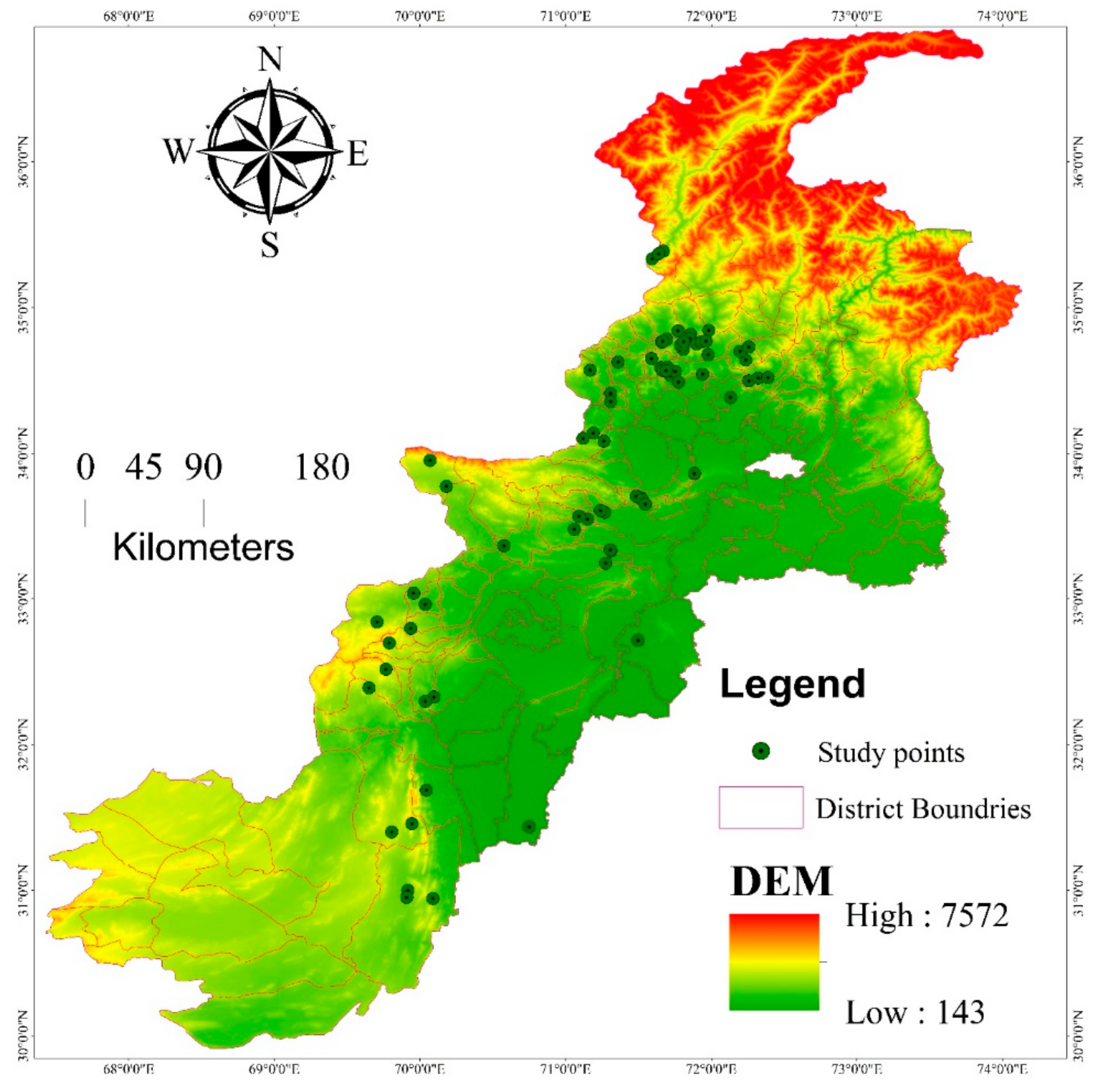
The vegetation diversity and carbon sequestration potential of M. buxifolia-dominated forests in its native region were studied at different localities across Pakistan during the period from 2018 to 2019 (Figure 1). Pakistan is a south Asian country spread on 80,943 km2 area, spinning between 60°55′ to 75°30′ of east longitude and 23°45′ to 36°50′ of north latitude [37]. Rough terrain, different valleys, steep slopes, large mountains, plains, deserts, and water tributaries linking rivers are the key characteristics of the studied area. Pakistan has a diverse climate and biodiversity due to the large altitudinal gradient ranging from sea level to 8611 m [43]. Pakistan has four distinct seasons, and the temperature varies both seasonally and regionally; the southern part has a hot and dry climate; the northwest has a temperate climate; the northern part is arctic [44]. Temperatures range from −22 °C in winter in the north to 50 °C in summer in the south. The precipitation is 1500–2000 mm and 100–200 mm across the north and south of Pakistan, respectively [45]. Pakistan is also going to face the brunt of climate change due to its hydrological reserve’s shrinkage, rapid glacier melting floods, and droughts [43]. The hotspot flora of the studied area is distributed in thirteen natural regions, i.e., Alpine pastures to Mangroves, where the endangered flora is >10% [46]. Phyto-geographically, Pakistan is divided into four regions (Indian region, Saharo-Indian region, Sino-Himalayan region and Irano-Turanian region) with the lowest diversity of plants in the Saharo-Sindian region covering a maximum portion of the country by area [43]. M. buxifolia populations are generally distributed at diverse elevation ranges and are often found to the west of the country.

Figure 1.
Map display 74 sampling locations of M. buxifolia dominated forests in different elevation ranges across Pakistan.
2.2. Data Collection and Field Inventory
In the study area, the major species of broadleaved forests are O. ferruginea, Quercus baloot, Acacia modesta, M. buxifolia, Punica granatum, etc. After going through a review of the literature and general survey, 74 least disturbed M. buxifolia-dominated forests spreads on more than 1 hectare area were selected for sampling following Phillips et al. [47]. The sampled forests were located on diverse altitudes with elevation ranging from 600 m to 1800 m asl. The sampled area was then divided into 3 elevation zones, i.e., Zone-I (600–999 m), Zone-II (1000–1399 m) and, Zone-III (1400–1799 m). In Zone-I and II, 26 sites were selected, while, in Zone-III, 22 sites were selected for sampling. In each sample site, 10 sample plots, each 15 m × 15 m and 5 m × 5 m were established for overstory and understory vegetation, respectively [36,37]. Within each plot, the diameters of all woody tree species were measured at breast height (DBH) following the protocol of Khan et al. [48]. In the case of multi-stem tree species, the diameters of all stems were measured separately, as suggested by Ali et al. [17]. DBH was measured with a diameter tape, while height (H, in m) was measured by a telescopic Hastings fiberglass rod (H < 15 m) (Hebei ShouChuang Composites Manufacturing Co., Ltd., Xingjianan Town, China) and Abneys level (made by Eugene Dietzgen Co., Chicago, IL, USA). Samples from tree species (parts), shrubs, and herbs (whole plant) were brought to the Botanical Garden Herbarium (BGH), University of Malakand, for identification.
2.3. Diversity Indices and Importance Value Index (IVI)
Within each sampling plot, importance values of individual woody tree species were calculated using relative values of frequency, density and basal area [39]. This synthetic index is recommended by several workers [3,5,37], as it reflects the degree of dominance, abundance and help in the conservation and management of a species [17]. To empirically measure the biodiversity, Alpha diversity in different stands was estimated by species richness indices (Margalef’s (DMg), Simpson’s (SI), Shannon-Wiener (ShWI) and Menhinick) in order to obtained a comparative quantitative estimate for compositional variability among different stands [49]. Such estimates are simple, easy to calculate and of great interest to ecologists and policy makers for various ecological settings [50].
2.4. Growing Stock Characteristics and Biomass Carbon Analysis
Several growing stock parameters for overstory vegetation, including density (ha−1), diameter (cm), height (m), basal area (BA m2 ha−1), and stand volume (m3 ha−1) were measured. Tree volume (m3 ha−1) of individual woody tree species was calculated following the standard methods of Philips et al. [47] by computing the given formula.
V = 0.5 × BA × H
We used the botanical identification of each individual to estimate wood density (WD), based on the information available in the scientific literature [17]. The given formula was utilized for obtaining stem biomass (SB) from the wood density and volume [51].
SB (T ha−1) = wood density (kg−3) × stem volume (m3 ha−1)
Similarly, total tree biomass (TB) was measured from SB and biomass expansion factor (BEF) using the given formula [51]:
Total TB (T ha−1) = stem biomass (T ha−1) × BEF
For understories vegetation, destructive sampling methods were used, wherein 15 individuals of each species were uprooted, and the fresh weight was measured. The samples were then oven-dried, and its dry weight was measured. From the cover and dry weight, we developed regression models; biomass was then calculated accordingly [35].
where Y = biomass of the species, Yo = 23.12, a = 0.84 and x = cover of the species.
The carbon stock in vegetation was assessed form the biomass. A conversion factor (0.5) was used to calculate total carbon density (ha−1) using the given formula [40,52];
Carbon Density (T ha−1) = Total TB (T ha−1) × 0.5
2.5. Soil Carbon Stock
Soil samples were collected from all the sampled plots to assess soil organic carbon (SOC) and soil bulk density (BD) at a depth of 20 cm. Rings of stainless steel (diameter = 14 and height = 20 cm) were vertically inserted for soil collection (manufacturer Huijian warehouse, Wuxi, China). After proper packing, the soil samples were then brought to the Agriculture Research Centre, Swat, for physiochemical analysis. The soil samples were oven-dried at 100 °C to a constant mass, weighed, crushed, and sieved (2 mm) to remove stones; then, they were weighed again. Bulk density of each sample was measured using the stone-free dry weight (g) and the steel ring volume (cm3). Soil organic matter (SOM) was determined using the volumetric method of Walkley and Black [53]. The soil organic carbon (% SOC) was measured by dividing SOM on 1.72 and the total soil carbon in T ha−1 was calculated following Ahmad et al. [40]. The following formula was computed:
where, SOC are the soil organic carbon (T ha−1), BD is the bulk density (g cm−3), D is the total depth at which the sample was taken (cm), and % SOC is the soil organic carbon concentration. Bulk density (BD) was derived following the procedure of Gebeyehu et al. [23].
2.6. Statistical Analysis
For biodiversity indices, an online calculator was used to measured species richness; diversity was estimated through different diversity indices [37]. The phytosociological attributes and absolute values were summarized following Ali et al. [17] and Khan et al. [36]. Importance values for individual tree species were calculated following Khan et al. [36]. Density (ha−1) and basal area m2 ha−1 were calculated for individual stands, pooled into groups; mean values were calculated. The data was statistically evaluated by SPSS (version 16), PAST and sigma plots. ANOVA and post hoc Tukey HSD tests were performed to highlight the difference between different elevation zones. Standard deviation (SD) and coefficient of variation (CV %) were calculated for the results. Regression models were used to figure out the link between different stand parameters like stem diameter (cm) and stem density (ha−1), tree height (m), tree basal area (m2 ha−1) and tree volume (m3 ha−1), tree basal (m2 ha−1) area and stem biomass (T ha−1).
3. Results
3.1. Forest Structure and Species Diversity
The study reported a total of 86 plant species belonging to 70 genera and 52 families in the phytocoenosis Monotheca forests.) Of the recorded flora, 31.4% (27 species) were from tree stratum and contributed 25 genera and 22 families, while the remaining 64.5% were shared by shrubs (38.4%), herbs (25.6%) and grasses (4.6%). Based on the importance value, M. buxifolia was recorded as the dominant tree species in the studied forests (Table 1). The importance value for the dominant species ranged from 52.57 to 100, with a mean value of 81.01 ± 2.8%. Zone-I occupied lower altitudes ranging from 600 m to 999 m asl where Acacia modesta (IV = 7.42 ± 2.23) was in strong association with the dominant species, followed by Olea ferruginea (IV = 2.58 ± 0.89) and Ziziphus muratiana (IV = 2.11 ± 0.98). Zone-II was located at the middle elevation, ranged from 1000 m to 1399 m asl and declared as a pure Monotheca community with a mean IVI of 85.52%, while all the remaining associated species show weak presence with importance value of less than 5. The community that occurred at higher elevation (Zone-III) were led by Monotheca with 81.63 ± 2.80 and O. ferruginea with 7.82 ± 2.20% of importance values. The presence of A. modesta and O. ferruginea with the dominant species in all three elevation zones highlights that these three broadleaved tree species are strong companions of each other. Apart from these three species, Ailanthus altissima, Dalbergia sissoo, and Eucalyptus globulus were the other major associates at lower elevation. In Zone-III, the strong co-dominant species was O. ferruginea; however, Pinus roxburghii, Juglans regia, and Punica granatum were recorded in comparatively weak association. Melia azedarach, Morus alba, Grewia oppositifolia, Acacia nilotica, Broussonetia papyrifera, and Albizia lebbeck were some of the other associates with dominant species.

Table 1.
Mean importance values indices (IVI), stem density ha−1 (D. ha−1) and Basal area m2 ha−1 (BA) of the tree species for Monotheca dominated forests across different elevation ranges in Pakistan.
The species richness and diversity indices for each elevation zone were calculated and are given in Table 2. Zone-I (Monotheca-Acacia) at lower elevation has the highest species richness (23 species) followed by Zone-II (18 species) and Zone-III, with 15 woody tree species. Monotheca phytocoenosis located at lower elevation shows high species diversity with a value of 1.52 ± 0.09 for Simpson’s Index (1/D) followed by the middle and high elevation groups (Table 2). Similar trend was also observed for Margalef’s Index (M), Shannon-Wiener Index (H’), and Pielou’s Index (J) diversity indices. One-way ANOVA was performed to determine the effect of altitudinal variations on species richness and diversity indices. The results reported significant difference between species richness and Simpsons’ index at p < 0.05 for all the three zones, which was further confirmed by performing a post-hoc Tukey HSD test (Table 2).
Table 2.
Species richness and diversity indices for the woody tree species in Monotheca forests communities across elevation ranges.
3.2. Structural Attributes and Growing Stock Volume
The growing stock volume of the dominant and all the associated species were calculated in each elevation zone. High number of individuals (317.70 trees ha−1), and basal area (67.56 m2 ha−1) were recorded for the stands at lower elevation ranges in which the dominant species shared 80.2% to density and 77.7% to basal area (Table 1). Forests of high elevation zones have a density of 290.93 trees ha−1 with basal area of 64.95 m2 ha−1. Community type present at middle elevation had least density (280.36 trees ha−1) and basal area (53.63 m2 ha−1) in comparison to other two groups due to human interference. The current study revealed that in the Monotheca dominated forests, the average height, basal area and average density varied significantly between different diameter classes (Table 3). The maximum mean height was recorded in diameter class-2 (8.03 m), while the lowest was found in class-5 (1.44 m). In similar fashion, the average mean density varied between 20.24 ha−1 for diameter class ranged from 25 to 44 cm to 94.71 ha−1 for the highest diameter class, whereas the basal area values were significantly higher for diameter class-3 (12.71 m2 ha−1) followed by class-4 (12.56 m2 ha−1) (Table 3). In the Monotheca phytocoenosis, volume (m3 ha−1) ranged from 26.30 to 54.12, wherein 24–44 cm diameter class shared 28.8% of the total volume followed by diameter class-2 with 21.9% volume. The mean volume for Zone-I was recorded maximum (78.09 m3 ha−1) followed by zone-III (61.89 m3 ha−1) and stands of Zone-II (48.01 m3 ha−1) located at lower altitudinal ranges as shown in Table 4. Similar trend was observed for stem biomass (T ha−1), total biomass (T ha−1), soil carbon and carbon stock (T ha−1).
Table 3.
Average height, Basal area and density of Monotheca in different diameter classes.
Table 4.
Total volume, stem biomass, tree biomass and carbon stock (T ha−1) of woody tree species, under story vegetation and soil 74 of Monotheca dominated forests across different elevation ranges in Pakistan.
3.3. Biomass and Carbon Stock
The mean stem biomass in the stands of lower elevation ranges (63.88 T ha−1) was significantly higher than stands of elevation zone-II (39.86 T ha−1) and zone-III (51.28 T ha−1). The dominant species shared 95% to the total stem biomass (Supplementary Materials Table S1). Among the other associates, Acacia modesta shared 1.71%, followed by Olea ferruginea (1.29%). The remaining 24 minor associates collectively shared 1.39% of the total stem biomass. A similar tendency was also recorded for total biomass with 66.85 T ha−1 for the lower elevation zone followed by stands the higher and middle altitudes, respectively. The current study also highlights the biomass carbon of all woody tree species (Table 4) and understories vegetation (Supplementary Materials Table S2) in three different elevation groups. In the tree stratum, the total amount of biomass carbon stock in lower elevation ranges was 51.81 T ha−1, of which the dominant (Monotheca) and co-dominant species (Acacia modesta) shared 95.6% and 2.6%, respectively. Ziziphus muratiana and Olea ferruginea were among the other major contributing species, adding 0.25 T ha−1 and 0.24 T ha−1 to the total carbon stock, respectively. Only 41.42 T ha−1 of carbon was calculated for the Monotheca-dominated forests located at high altitudinal ranges, while this value is lowest for group-II (31.95 T ha−1), located at elevation range from 1000 m to 1399 m asl (Table 4). Likewise, an increasing trend of soil carbon (T ha−1) was also observed along the altitudinal gradient. Understory vegetation in each altitudinal range mainly consisted of grasses, herbs, and shrubs. Among grasses, Saccharum munja, Saccharum spontaneum, Sorghum halepense, and Cenchrus spinifex were more common, while major shrubs were Dodonaea viscosa, Justicia adhatoda, Cotoneaster microphyllus, Ziziphus nummularia and Ricinus communis. The mean carbon stocks of understory vegetation at lower altitudinal ranges were maximum (0.148 T ha−1) followed by middle and higher elevation ranges with values of 0.107 T ha−1 and 0.087 T ha−1, respectively.
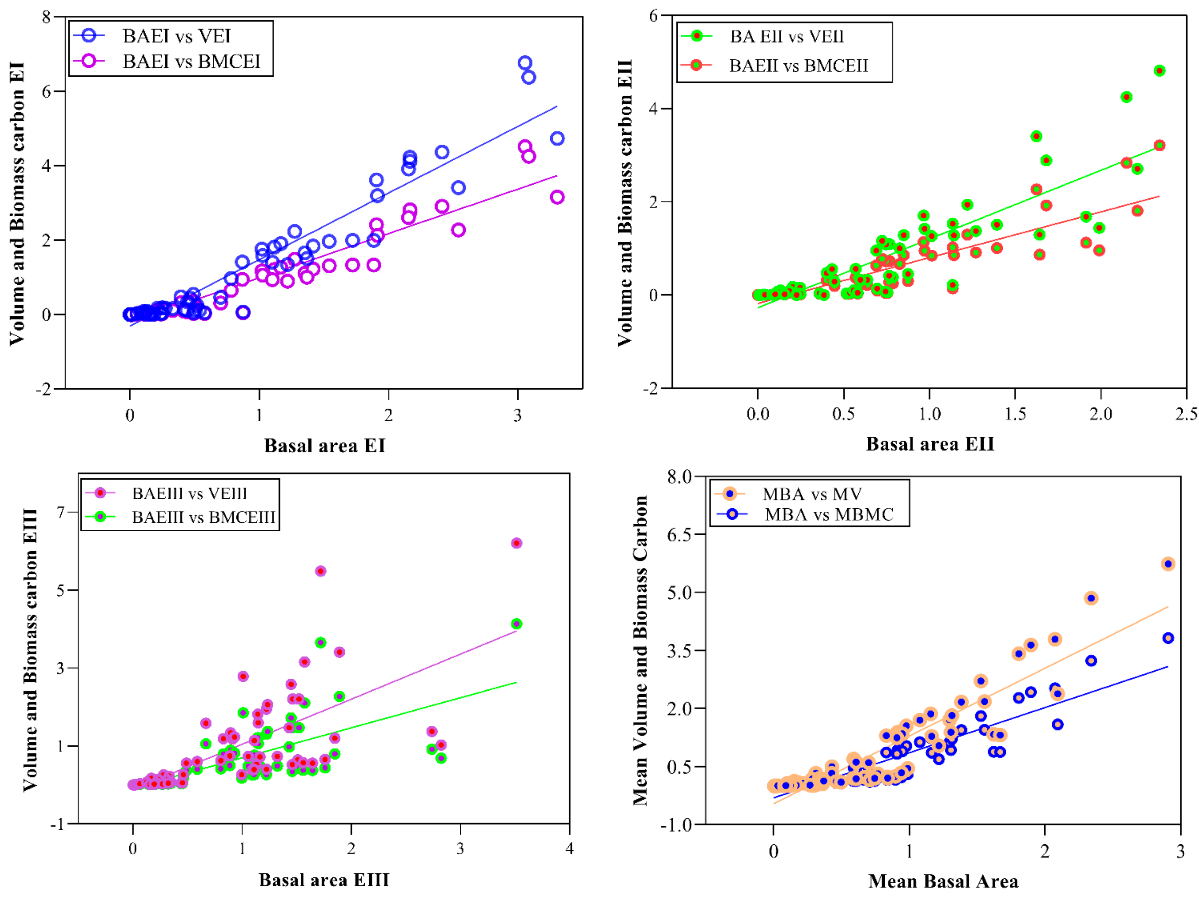
Stem density, stem volume, and biomass carbon are the functions of Basal area. Stem density decreases with increasing diameter, while stem volume and biomass carbon are in direct relation with diameter. To study the relationship between stem density, stem volume, and biomass carbon with diameter (cm), regression models were developed (Figure 2 and Figure 3). The model showed a strong relation (R2 = 0.55, 0.59 and 0.51) of density for lower, middle and higher altitudinal ranges, respectively. Overall, the relationship of stem density (ha−1) and diameter (cm) is quadratic type (polynomial inverse 3rd order) showing a significant value of R2 = 0.57 (Table 5). Similarly, the relationship of volume and biomass carbon with Basal area can be explained by the adjusted R2 values (0.92, 0.79 and 0.76) from lower to higher altitudinal ranges, respectively. In lower ranges, the volume was significantly correlated with Basal area, followed by middle and high elevation ranges. A similar trend was also observed in the relationship between biomass carbon and Basal area using quadratic regression type (R2 = 0.79).
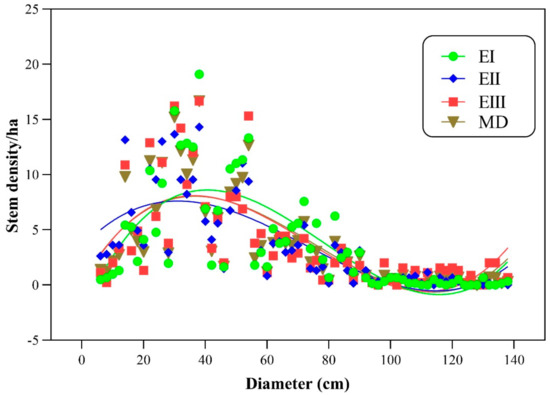
Figure 2.
Relation between stem density (ha−1) and diameter (cm). Note. DEI = density at elevation zone-I, DEII = density at elevation zone-II, DEIII = density at elevation zone-III, MD = mean density.
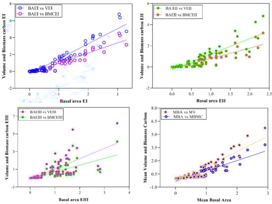
Figure 3.
Relationships between Basal area with volume and biomass carbon along different altitudinal gradients. Note. BAEI = Basal area at elevation zone-I, BAEII = Basal area at elevation zone-II, BAEI = Basal area at elevation zone-III, MBA = Mean basal area, VEI = Volume at elevation zone-I, VEII = Volume at elevation zone-II, VEIII = Volume at elevation zone-III, MV = Mean volume, BMCEI = Biomass carbon at elevation zone-I, BMCEII = Biomass carbon at elevation zone-II, BMCEIII = Biomass carbon at elevation zone-III, MBMC = Mean biomass carbon.
Table 5.
Regression equation explaining the relation of different parameters.
4. Discussion
The forests of Pakistan, like other vegetation types, has variation in species composition and diversity due to topographic and edaphic variables. The current study outlines three major phytocoenosis of Monotheca buxifolia at different altitudinal ranges. The presence of M. buxifolia as a dominant species with varying stem density explains the wide distribution of the species in the studied area. These results are more similar to the findings of Khan et al. [38,39], by reporting M. buxifolia as a dominant tree species in the studied area. Prominent existence of this species was also observed by Ali et al. [37] and Khan et al. [54], working on Olea ferruginea and Quercus baloot vegetation, respectively. O. ferruginea and Acacia modesta were strong associates of the dominant species, with importance values that ranged from 2.40 ± 1.28 to 7.82 ± 2.20%. The remaining 24 species, including Morus alba, Ficus palmata, Broussonetia papyrifera, Juglans regia, Pinus roxburghii, etc., were poorly distributed (importance value 0.11 ± 0.11 to 2.11 ± 0.98%). Pinus gerardiana, Prunus armeniaca, Pinus roxburghii, Phoenix dactylifera, and Punica granatum were positioned in high elevation, while Dalbergia sissoo, Acacia nilotica, Albizia lebbeck and Capparis decidua were more familiar in lower elevation. Morus alba, Melia azedarach, Ficus palmata, Ailanthus altissima, Grewia oppositifolia, and Populus nigra were found in both lower and upper elevations. The distribution pattern of tree species in Monotheca phytocoenosis can be strongly linked with the findings of Khan et al. [36] and Ali et al. [37]. Exotic species such as E. globulus, B. papyrifera, and A. altissima are introduced by locals and have negative ecological consequences for native species [55]. Removal of the invasive plants is highly recommended from the natural population for successful forest resource management [36].
Results of ANOVA and post hoc Tukey HSD revealed that Simpson index and richness of lower elevation had the highest diversity in comparison to middle and high elevation ranges. Log series and Margalef’s index had the same result: high diversity for lower elevation followed by higher elevation (Table 2). Data was collected at three different altitudinal ranges; forests at low elevation ranges were more dense and diverse. However, those forests which were located at higher altitudinal ranges are comparatively scarce. Decline in the tree density, basal area, and species richness with increasing altitude is significant in Himalayan forests [15,56]. The current study observed a significant loss in vegetation along the altitudinal strata due to eco-physiological constraints, low temperature, and productivity [57]. In terms of the association between species diversity and elevation gradient, the current study supports the existing literature [17,36,37]. Our results suggest that being highly diversified holds a significant relationship with elevation. This may be attributed to several factors, such as temperature, precipitation, soil properties, and intensity of disturbance. The favorable association between plant species richness and altitudinal gradient has already been proven in various studies [4,58,59]; it revealed that species richness is highly influenced by altitudinal linked factors [60]. This could be true in a controlled setting free of anthropogenic and other natural disruptions.
Different tree variables, such as tree type, height, basal area, stem volume, etc. determines the nature of forest community and growing stock characteristics of the forests. Growing stock-based estimation of biomass and carbon stock are reliable and valuable sources [40,41]. The current study reported stem density of 317.70 ha−1 at lower altitudinal ranges followed by higher and mid-elevation ranges with values of 290.93 ha−1 and 280.36 ha−1, respectively, which is quite within the range of Khan et al. [37] but lower from the findings of Ali et al. [17]. The recorded stem density in the current work is in line with the expected range (133 to 620 trees ha−1) from a different region of Pakistan, as documented by Ahmed et al. [61]. In contrast to this result, Nizami et al. [51] documented low stem density while working on carbon stocks of subtropical forests from the same region. The present stem volume of 62.69 m3 ha−1 in Monotheca-dominant forests is comparable to the estimated volume of Olea ferruginea [37] but lower from the findings of Ahmad et al. [41]. Generally, the numbers of small diameter trees are much higher in comparison to larger diameter trees [36].
Altitude highly influences the ecosystem structure, composition, and biomass by altering different factors of the environment, including precipitation, temperature, slope, aspect, soil properties, etc. [62]. In this sense, the main aim of our study was to expose the impact of altitude on vegetation and soil organic carbon. Soil carbon is an integral part of a particular ecosystem. Several different factors like length of time, vegetation type physical and biological condition of soil significantly affect the carbon sequestration capacity of soil [63]. During the current work, SOC (T ha−1) were reported in increasing order with the altitude. Zone-I, located at a lower elevation, documented 16.69 T ha−1, Zone-II at mid elevation reported 24.53 T ha−1, while the Zone-III, presented at high altitude, recorded maximum values of SOC (36.21 T ha−1). A similar increasing pattern was also documented by Devi and Sherpa [58], which is in agreement with the present study. In contrast to the present study, SOC (T ha−1) was reported in a decreasing manner along the altitude gradient in various soil carbon studies [64,65,66]. This decreasing pattern of carbon was associated with a slow mineralization and nitrification process at the higher elevation. The increasing tendency of carbon with increasing altitude in our study could be due to greater SOC (T ha−1) stability at higher elevation ranges. Wood harvest effects the soil carbon as it reduces the amount of litter production [40]. In our study, the forests located at lower elevation are more prone to local communities for wood harvest, due to which a smaller amount of litter and resulting carbon stock is available at lower elevation as compared to higher elevation.
In the current study, we studied the relationship between stem density and diameter by developing regression models (polynomial cubic, Figure 2). Adjusted R2 for the middle elevation was 0.59, followed by lower elevation (R2 = 0.55) and higher elevation (R2 = 0.51), showing the presence of numerous individuals in the small diameter classes. We investigated the link of stem diameter to stem density (Figure 3) by polynomial cubic, where R2 = 0.57 shows the positive significant relationship. Tree diameter is a prominent and measurable variable for tree Basal area, as trees having a greater diameter will have a high Basal area. The presence of large girth trees in Monotheca forests resulted in high Basal area in comparison to the finding of Nizami et al. [67]. However, the current Basal area (10–26 m2 ha−1) supports the results of Ahmed et al. [61].
The potential of forests to store and sink atmospheric carbon for the long-term is highly affected by altitudinal gradients [62]. Growth conditions, species structure and composition, and other disturbance factors may all play a role in the carbon storing capacity of these forests [17]. Estimation of total biomass of forests in the current climate change scenario has received attention as the world is facing an increase in temperature; the forests are the only source to cope with this tension. The tree biomass and carbon in a forest is highly influenced by tree type, forest structure, tree diameter, tree age, precipitation, stand condition, and different topographic and edaphic variables [68]. Wani et al. [13] recorded a positive but weak relationship (R2 = 0.02) between aboveground biomass carbon and elevation (m, asl). In a similar study, Li et al. [19] found a strong positive relation (R2 = 0.57) of biomass carbon with elevation. Moreover, Liu and Nan [4] also reported the direct dependency of carbon stock and altitude across three forests of Loess Plateau (China). The possible reasons for such relations are the variation in temperature along the altitudinal gradient [13,19]. However, in contrast, lower biomass at high elevation ranges was also documented by several workers [69,70,71]. Sun et al. [72] reported a strong positive relation (R2 = 0.67) of ABG biomass with elevation in the central highland, Vietnam. Furthermore, the findings of Li et al. [19] exposes no significant interaction of altitude with vegetation carbon stock in Chitteri reserve forest.
Several studies reported a reduction in the amount of aboveground biomass with an increasing trend in elevation [73,74,75], while some of the workers reported the opposite scenario, i.e., an increase in biomass and carbon with an increase in altitude [76,77]. The current findings exposed an uneven trend in the amount of vegetation biomass and carbon along the altitudinal gradient; however, soil carbon was reported with an increasing pattern along the elevation. It could possibly be linked to the geographical aspect of the area, where the nearly-steep slope has isolated itself from continued interaction. These results are matched with the findings of Padmakumar et al. [28]; however, the reports of Phillips et al. [45] offer a visible challenge. One of the possible reasons for such a pattern is the presence of fewer but larger diameter trees at higher elevation. However, these findings disagree with previous results, which highlighted that mid altitude had the highest AGC [78,79]. The current study reported a variation in major carbon-storing tree species along the differed altitudinal zones. Tree species with wood density and greater DBH have the potential to contribute more biomass and can store more atmospheric carbon.
5. Conclusions
We studied species diversity, growing stock variables and carbon mitigation potential in the phytocoenosis of an evergreen broadleaved Monotheca buxifolia forest along its altitudinal gradient across the landscape in Pakistan. In this study, overall, 86 plant species belonging to 70 genera and 52 families were prevailing. The biomass and carbon stock varied significantly across the three elevation zones, where species richness, diversity and anthropogenic disturbances play a key role and are generally accountable for such marked variations. Tree biomass ranged from 63.90 T ha−1 in zone-II to 103.6 T ha−1 in zone-I. The total carbon stock for vegetation ranged from 32.05 T ha−1 to 51.95 32.05 T ha−1, while the soil carbon ranged from 16.69 T ha−1 in lower elevation to 36.21 T ha−1 at higher elevation ranges. The SOC had a strong positive relationship with elevation; in contrast, the vegetation carbon stock was recorded as minimum in the middle altitudinal ranges. The reasons for this pattern might be the disturbance regimes, species girth, and stand age. The uneven distribution of biomass and vegetation carbon stock over elevation contradicts several previous research studies that found a smooth trend, making this study distinctive and offering perceptions for further study. The current study was the first of its kind in evaluating biomass and carbon in the Monotheca-dominated forests of Pakistan in veins to the altitudinal gradient. Despite the miserable condition, these unmanaged forests sink a significant amount of carbon, which is critically essential for climate change mitigation in order to reduce global warming and its resulting effects. Presently, the forests are in decline and heading towards the extinction of its remaining green patches; therefore, instant conservation policies needs to be implemented.
Supplementary Materials
The following are available online at https://www.mdpi.com/article/10.3390/app12031292/s1, Table S1: Carbon stock (T ha−1) of woody tree species of Monotheca dominated forests across different elevation ranges in Pakistan, Table S2: Carbon stock (T ha−1) of understories vegetation of Monotheca dominated forests across different elevation ranges in Pakistan.
Author Contributions
F.A. is involved in field data collection and preparation of the preliminary draft. A.A. is involved in statistical analyses, E.F.A. is involved in the revision and finalization of this manuscript. N.K. developed the study design, and did the supervision of all research activities. All authors have read and agreed to the published version of the manuscript.
Funding
The authors would like to extend their sincere appreciation to the Researchers Supporting Project Number (RSP-2021/134), King Saud University, Riyadh, Saudi Arabia.
Data Availability Statement
The data presented in this study are available on request from the corresponding author.
Acknowledgments
The authors would like to extend their sincere appreciation to the Researchers Supporting Project Number (RSP-2021/134), King Saud University, Riyadh, Saudi Arabia.
Conflicts of Interest
The authors declare no conflict of interest.
References
- Arasa-Gisbert, R.; Vayreda, J.; Román-Cuesta, R.M.; Villela, S.A.; Mayorga, R.; Retana, J. Forest diversity plays a key role in determining the stand carbon stocks of Mexican forests. For. Ecol. Manag. 2018, 415, 160–171. [Google Scholar] [CrossRef]
- Zhang, Y.; Gu, F.; Liu, S.; Liu, Y.; Li, C. Variations of carbon stock with forest types in subalpine region of southwestern China. For. Ecol. Manag. 2013, 300, 88–95. [Google Scholar] [CrossRef]
- Aryal, S.; Shrestha, S.; Maraseni, T.; Wagle, P.C.; Gaire, N.P. Carbon stock and its relationships with tree diversity and density in community forests in Nepal. Int. For. Rev. 2018, 20, 263–273. [Google Scholar] [CrossRef]
- Liu, N.; Nan, H. Carbon stocks of three secondary coniferous forests along an altitudinal gradient on Loess Plateau in inland China. PLoS ONE 2018, 13, e0196927. [Google Scholar] [CrossRef] [PubMed] [Green Version]
- Badshah, M.T.; Ahmad, A.; Muneer, M.A.; Rehman, A.U.; Wang, J.; Khan, M.; Muhammad, B.; Amir, M.; Meng, J. Evaluation of the forest structure, diversity and biomass carbon potential in the southwest region of Guangxi, China. Appl. Ecol. Environ. Res. 2017, 18, 447–467. [Google Scholar] [CrossRef]
- Rajput, B.S.; Bhardwaj, D.R.; Pala, N.A. Factors influencing biomass and carbon storage potential of different land use systems along an elevational gradient in temperate northwestern Himalaya. Agrofor. Syst. 2017, 91, 479–486. [Google Scholar] [CrossRef] [Green Version]
- Sharma, C.M.; Gairola, S.; Baduni, N.P.; Ghildiyal, S.K.; Suyal, S. Variation in carbon stocks on different slope aspects in seven major forest types of temperate region of Garhwal Himalaya, India. J. Biosci. 2011, 36, 701–708. [Google Scholar] [CrossRef] [PubMed]
- Simegn, T.Y.; Soromessa, T. Carbon stock variations along altitudinal and slope gradient in the forest belt of Simen Mountains National Park, Ethiopia. Am. J. Environ. Prot. 2015, 4, 199–201. [Google Scholar] [CrossRef] [Green Version]
- Curtis, J.T.; Mcintosh, R.P. The interrelations of certain analytic and synthetic phytosociological characters. Ecology 1950, 31, 434–455. [Google Scholar] [CrossRef]
- Khan, K.; Iqbal, J.; Ali, A.; Khan, S.N. Assessment of Sentinel-2-Derived Vegetation Indices for the Estimation of Above-Ground Biomass/Carbon Stock, Temporal Deforestation and Carbon Emissions Estimation in the Moist Temperate Forests of Pakistan. Appl. Ecol. Environ. Res. 2020, 18, 783–815. [Google Scholar] [CrossRef]
- Ma, J.; Bu, R.; Liu, M.; Chang, Y.; Qin, Q.; Hu, Y. Ecosystem carbon storage distribution between plant and soil in different forest types in Northeastern China. Ecol. Eng. 2015, 81, 353–362. [Google Scholar] [CrossRef]
- Naudts, K.; Chen, Y.; McGrath, M.J.; Ryder, J.; Valade, A.; Otto, J.; Luyssaert, S. Europe’s forest management did not mitigate climate warming. Science 2016, 351, 597–600. [Google Scholar] [CrossRef] [PubMed]
- Wani, A.A.; Bhat, A.F.; Gatoo, A.A.; Zahoor, S.; Mehraj, B.; Mir, N.A.; Masoodi, T.H. Relationship of forest biomass carbon with biophysical parameters in north Kashmir region of Himalayas. Environ. Monit. Assess. 2019, 191, 1–13. [Google Scholar] [CrossRef]
- Anonymous. Global Forest Resource Assessments; Forestry Paper No: 163; FAO: Rome, Italy, 2010. [Google Scholar]
- Gairola, S.; Sharma, C.M.; Ghildiyal, S.K.; Suyal, S. Live tree biomass and carbon variation along an altitudinal gradient in moist temperate valley slopes of the Garhwal Himalaya (India). Curr. Sci. 2011, 100, 1862–1870. [Google Scholar]
- Khadanga, S.S.; Jayakumar, S. Tree biomass and carbon stock: Understanding the role of species richness, elevation, and disturbance. Trop. Ecol. 2020, 61, 128–141. [Google Scholar] [CrossRef]
- Ali, F.; Khan, N.; Ahmad, A.; Khan, A.A. Structure and biomass carbon of Olea ferruginea forests in the foot hills of Malakand division, Hindukush Range Mountains of Pakistan. Acta Ecol. Sin. 2019, 39, 261–266. [Google Scholar] [CrossRef]
- Yang, B.; Zhang, W.; Lu, Y.; Zhang, W.; Wang, Y. Carbon storage dynamics of secondary forest succession in the central Loess Plateau of China. Forests 2019, 10, 342. [Google Scholar] [CrossRef] [Green Version]
- Li, J.; Chen, Q.; Li, Z.; Peng, B.; Zhang, J.; Xing, X.; Zhao, B.; Song, D. Distribution and altitudinal patterns of carbon and nitrogen storage in various forest ecosystems in the central Yunnan Plateau, China. Sci. Rep. 2021, 11, 6269. [Google Scholar] [CrossRef] [PubMed]
- Cao, B.; Domke, G.M.; Russell, M.B.; Walters, B.F. Spatial modeling of litter and soil carbon stocks on forest land in the conterminous United States. Sci. Total Environ. 2019, 654, 94–106. [Google Scholar] [CrossRef]
- FAO. Global Forest Resources Assessment 2015: How Are the World’s Forests Changing? 2nd ed.; Food and Agriculture Organization of the United Nations: Rome, Italy, 2016; pp. 1–44. [Google Scholar]
- Sharma, P.; Rai, S.C. Carbon sequestration with land-use cover change in a Himalayan watershed. Geoderma 2007, 139, 371–378. [Google Scholar] [CrossRef]
- Gebeyehu, G.; Soromessa, T.; Bekele, T.; Teketay, D. Carbon stocks and factors affecting their storage in dry Afromontane forests of Awi Zone, northwestern Ethiopia. J. Ecol. Environ. 2019, 43, 17. [Google Scholar] [CrossRef] [Green Version]
- Liang, C.; Schimel, J.P.; Jastrow, J.D. The importance of anabolism in microbial control over soil carbon storage. Nat. Microbiol. 2017, 2, 17105. [Google Scholar] [CrossRef] [PubMed]
- Thom, D.; Golivets, M.; Edling, L.; Meigs, G.W.; Gourevitch, J.D.; Sonter, L.J.; Galford, G.L.; Keeton, W.S. The climate sensitivity of carbon, timber, and species richness covaries with forest age in boreal–temperate North America. Glob. Chang. Biol. 2019, 25, 2446–2458. [Google Scholar] [CrossRef] [PubMed]
- Sharma, C.M.; Tiwari, O.P.; Rana, Y.S.; Krishan, R.; Mishra, A.K. Elevational behaviour on dominance–diversity, regeneration, biomass and carbon storage in ridge forests of Garhwal Himalaya, India. For. Ecol. Manag. 2018, 424, 105–120. [Google Scholar] [CrossRef]
- Cha, J.Y.; Cha, Y.; Oh, N.H. The effects of tree species on soil organic carbon content in South Korea. J. Geophys. Res. Biogeosci. 2019, 124, 708–716. [Google Scholar] [CrossRef]
- Padmakumar, B.; Sreekanth, N.P.; Shanthiprabha, V.; Paul, J.; Sreedharan, K.; Augustine, T.; Jayasooryan, K.K.; Rameshan, M.; Arunbabu, V.; Mohan, M.; et al. Unveiling tree diversity and carbon density of homegarden in the Thodupuzha urban region of Kerala, India: A contribution towards urban sustainability. Trop. Ecol. 2021, 62, 508–524. [Google Scholar] [CrossRef]
- Babweteera, F.; Plumptre, A.J.; Adamescu, G.S.; Shoo, L.P.; Beale, C.M.; Reynolds, V.; Nyeko, P.; Muhanguzi, G. The ecology of tree reproduction in an African medium altitude rain forest. Biotropica 2018, 50, 405–417. [Google Scholar] [CrossRef] [Green Version]
- Chave, J.; Réjou-Méchain, M.; Búrquez, A.; Chidumayo, E.; Colgan, M.S.; Delitti, W.B.; Duque, A.; Eid, T.; Fearnside, P.M.; Goodman, R.C.; et al. Improved allometric models to estimate the aboveground biomass of tropical trees. Glob. Chang. Biol. 2014, 20, 3177–3190. [Google Scholar] [CrossRef]
- Chinasho, A.; Soromessa, T.; Bayable, E. Carbon stock in woody plants of Humbo forest and its variation along altitudinal gradients: The case of Humbo district, Wolaita zone, southern Ethiopia. Int. J. Environ. Prot. Policy 2015, 3, 97–103. [Google Scholar] [CrossRef] [Green Version]
- Charan, G.; Bharti, V.K.; Jadhav, S.E.; Kumar, S.; Angchok, D.; Acharya, S.; Srivastava, R.B. Altitudinal variations in soil carbon storage and distribution patterns in cold desert high altitude microclimate of India. Afr. J. Agric. Res. 2012, 7, 6313–6319. [Google Scholar] [CrossRef]
- Chaturvedi, R.K.; Raghubanshi, A.S. Assessment of carbon density and accumulation in mono-and multi-specific stands in Teak and Sal forests of a tropical dry region in India. For. Ecol. Manag. 2015, 339, 11–21. [Google Scholar] [CrossRef]
- Chisanga, K.; Bhardwaj, D.R.; Pala, N.A.; Thakur, C.L. Biomass production and carbon stock inventory of high-altitude dry temperate land use systems in North Western Himalaya. Ecol. Processes 2018, 7, 22. [Google Scholar] [CrossRef]
- Van Do, T.; Sato, T.; Dai Hai, V.; Thang, N.T.; Binh, N.T.; Son, N.H.; Van Thuyet, D.; Van, T.; Hung, T.T.; Van, C.; et al. Aboveground biomass and tree species diversity along altitudinal gradient in Central Highland, Vietnam. Trop. Ecol. 2017, 58, 95–104. [Google Scholar]
- Khan, A.A.; Ali, F.; Ihsan, M.; Hayat, K.; Nabi, G. Ethnobotanical study of the medicinal plants of Tehsil Charbagh, district Swat, Khyber Pakhtunkhwa, Pakistan. Am. Eurasian J. Agric. Environ. Sci. 2015, 15, 1464–1474. [Google Scholar] [CrossRef]
- Ali, F.; Khan, N.; Ali, K.; Khan, I. Influence of environmental variables on the distribution of woody species in Muslim graveyards of Malakand Division, Hindukush Range Mountains of Pakistan. Pak. J. Bot. 2017, 49, 2357–2366. [Google Scholar]
- Khan, N.; Ahmed, M.; Shaukat, S.S.; Wahab, M.; Siddiqui, M.F. Structure, diversity, and regeneration potential of Monotheca buxifolia (Falc.) A. DC. dominated forests of Lower Dir District, Pakistan. Front. Agric. China 2011, 5, 106–121. [Google Scholar] [CrossRef]
- Khan, N.; Ahmed, M.; Wahab, M.; Ajaib, M.; Hussain, S.S. Studies along an altitudinal gradient in Monotheca buxifolia (falc.) ad, forest, District Lower Dir, Pakistan. Pak. J. Bot. 2010, 42, 3029–3038. [Google Scholar]
- Ahmad, A.; Liu, Q.J.; Nizami, S.M.; Mannan, A.; Saeed, S. Carbon emission from deforestation, forest degradation and wood harvest in the temperate region of Hindukush Himalaya, Pakistan between 1994 and 2016. Land Use Policy 2018, 78, 781–790. [Google Scholar] [CrossRef]
- Abbas, M.; Nizami, S.M.; Saleem, A.; Gulzar, S.; Khan, I.A. Biomass expansion factors of Olea ferruginea (Royle) in subtropical forests of Pakistan. Afr. J. Biotechnol. 2011, 10, 1586–1592. [Google Scholar] [CrossRef]
- Ahmad, A.; Nizami, S.M. Carbon stocks of different land uses in the Kumrat valley, Hindu Kush Region of Pakistan. J. For. Res. 2015, 26, 57–64. [Google Scholar] [CrossRef]
- Ali, S.I.; Qaiser, M. A phytogeographical analysis of the phanerogams of Pakistan and Kashmir. Proc. R. Soc. Edinb. Sect. B Biol. Sci. 1986, 89, 89–101. [Google Scholar] [CrossRef]
- Huang, J.; Ji, M.; Xie, Y.; Wang, S.; He, Y.; Ran, J. Global semi-arid climate change over last 60 years. Clim. Dyn. 2016, 46, 1131–1150. [Google Scholar] [CrossRef] [Green Version]
- Hussain, F.; Nabi, G.; Wu, R.S. Spatiotemporal Rainfall Distribution of Soan River Basin, Pothwar Region, Pakistan. Adv. Meteorol. 2021, 12, 973. [Google Scholar] [CrossRef]
- Shinwari, Z.K.; Qaiser, M. Efforts on conservation and sustainable use of medicinal plants of Pakistan. Pak. J. Bot. 2011, 43, 5–10. [Google Scholar]
- Phillips, J.; Ramirez, S.; Wayson, C.; Duque, A. Differences in carbon stocks along an elevational gradient in tropical mountain forests of Colombia. Biotropica 2019, 51, 490–499. [Google Scholar] [CrossRef]
- Khan, N.; Ali, F.; Ali, K.; Shaukat, S. Composition, structure and regeneration dynamics of Olea ferruginea Royle forests from Hindukush range of Pakistan. J. Mt. Sci. 2015, 12, 647–658. [Google Scholar] [CrossRef]
- Pielou, E.C. An Introduction to Mathematical Ecology, 2nd ed.; Wiley-Interscience: Hoboken, NJ, USA, 1969; pp. 1–286. [Google Scholar]
- Purvis, A.; Hector, A. Getting the measure of biodiversity. Nature 2000, 405, 212–219. [Google Scholar] [CrossRef]
- Nizami, S.M. The inventory of the carbon stocks in subtropical forests of Pakistan for reporting under Kyoto Protocol. J. For. Res. 2012, 23, 377–384. [Google Scholar] [CrossRef]
- Andersson, K.; Evans, T.P.; Richards, K.R. National forest carbon inventories: Policy needs and assessment capacity. Clim. Change 2009, 93, 69–101. [Google Scholar] [CrossRef]
- Walkley, A.; Black, I.A. An examination of the Degtjareff method for determining soil organic matter, and a proposed modification of the chromic acid titration method. Soil Sci. 1934, 37, 29–38. [Google Scholar] [CrossRef]
- Khan, N.; Ahmed, M.; Wahab, M.; Ajaib, M. Phytosociology, structure and physiochemical analysis of soil in Quercus baloot Griff, Forest District Chitral Pakistan. Pak. J. Bot. 2011, 42, 2429–2441. [Google Scholar]
- Nunes, L.J.; Raposo, M.A.; Meireles, C.I.; Pinto Gomes, C.J.; Almeida Ribeiro, N. Carbon Sequestration Potential of Forest Invasive Species: A Case Study with Acacia dealbata Link. Resources 2021, 10, 51. [Google Scholar] [CrossRef]
- Vellend, M.; Harmon, L.J.; Lockwood, J.L.; Mayfield, M.M.; Hughes, A.R.; Wares, J.P.; Sax, D.F. Effects of exotic species on evolutionary diversification. Trends Ecol. Evol. 2007, 22, 481–488. [Google Scholar] [CrossRef] [PubMed]
- Gathorne-Hardy, F.; Syaukani; Eggleton, P. The effects of altitude and rainfall on the composition of the termites (Isoptera) of the Leuser Ecosystem (Sumatra, Indonesia). J. Trop. Ecol. 2001, 17, 379–393. [Google Scholar] [CrossRef]
- Devi, S.B.; Sherpa, S. Soil carbon and nitrogen stocks along the altitudinal gradient of the Darjeeling Himalayas, India. Environ. Monit. Assess. 2019, 191, 361. [Google Scholar] [CrossRef] [PubMed]
- Deresa, A. Carbon Stock Estimation Along Altitudinal Gradient in Woodland Vegetation in Ilu Gelan District, West Shewa Zone of Oromia Region, Central Ethiopia. Ph.D. Thesis, Addis Ababa University, Addis Ababa, Ethiopia, 2015. [Google Scholar]
- Mwakisunga, B.; Majule, A.E. The influence of altitude and management on carbon stock quantities in rungwe forest, southern highland of Tanzania. Open J. Ecol. 2012, 2, 214–221. [Google Scholar] [CrossRef] [Green Version]
- Ahmed, M.; Husain, T.; Sheikh, A.H.; Hussain, S.S.; Siddiqui, M.F. Phytosociology and structure of Himalayan forests from different climatic zones of Pakistan. Pak. J. Bot. 2006, 38, 361. [Google Scholar]
- Alves, L.F.; Vieira, S.A.; Scaranello, M.A.; Camargo, P.B.; Santos, F.A.; Joly, C.A.; Martinelli, L.A. Forest structure and live aboveground biomass variation along an elevational gradient of tropical Atlantic moist forest (Brazil). For. Ecol. Manag. 2010, 260, 679–691. [Google Scholar] [CrossRef]
- Post, W.M.; Kwon, K.C. Soil carbon sequestration and land-use change: Processes and potential. Glob. Change Biol. 2000, 6, 317–327. [Google Scholar] [CrossRef] [Green Version]
- Mishra, A.K.; Singh, K.; Behera, S.K.; Chaudhary, L.B.; Singh, B.; Mishra, R.M. Soil properties in response to different plant community structures in tropical moist deciduous forest from Northern India. Clim. Change Environ. Sustain. 2017, 5, 66–74. [Google Scholar] [CrossRef]
- Krishnan, P.; Bourgeon, G.; Seen, D.L.; Nair, K.M.; Prasanna, R.; Srinivas, S.; Muthusankar, G.; Dufy, L.; Ramesh, B.R. Organic carbon stock map for soils of southern India: A multifactorial approach. Curr. Sci. 2007, 93, 706–710. [Google Scholar]
- Sheikh, M.A.; Kumar, M.; Bussmann, R.W. Altitudinal variation in soil organic carbon stock in coniferous subtropical and broadleaf temperate forests in Garhwal Himalaya. Carbon Balance Manag. 2009, 4, 6. [Google Scholar] [CrossRef] [PubMed] [Green Version]
- Nizami, S.M.; Mirza, S.N.; Livesley, S.; Arndt, S.; Fox, J.C.; Khan, I.A.; Mahmood, T. Estimating carbon stocks in sub-tropical pine (Pinus roxburghii) forests of Pakistan. Pak. J. Agri. Sci. 2009, 46, 266–270. [Google Scholar]
- Ullah, S.; Khan, N.; Ali, F.; Badshah, L.; Ali, A.; Muhammad, M. An ecological assessment of Justicia adhatoda L. in Malakand Division, Hindukush range of Pakistan. Biosci. Res. 2020, 17, 1082–1094. [Google Scholar]
- Srinivas, K.; Sundarapandian, S. Biomass and carbon stocks of trees in tropical dry forest of East Godavari region, Andhra Pradesh, India. Geol. Ecol. Lands 2019, 3, 114–122. [Google Scholar] [CrossRef]
- Bangroo, S.A.; Najar, G.R.; Rasool, A. Effect of altitude and aspect on soil organic carbon and nitrogen stocks in the Himalayan Mawer Forest Range. Catena 2017, 158, 63–68. [Google Scholar] [CrossRef]
- Zhu, B.; Wang, X.; Fang, J.; Piao, S.; Shen, H.; Zhao, S.; Peng, C. Altitudinal changes in carbon storage of temperate forests on Mt Changbai, Northeast China. J. Plant Res. 2010, 123, 439–452. [Google Scholar] [CrossRef] [PubMed]
- Sun, L.; Wang, M.; Fan, X. Spatial pattern and driving factors of biomass carbon density for natural and planted coniferous forests in mountainous terrain, eastern Loess Plateau of China. For. Ecosyst. 2020, 7, 9. [Google Scholar] [CrossRef] [Green Version]
- Naveenkumar, J.; Arunkumar, K.S.; Sundarapandian, S.M. Biomass and carbon stocks of a tropical dry forest of the Javadi Hills, Eastern Ghats, India. Carbon Manag. 2017, 8, 351–361. [Google Scholar] [CrossRef]
- Moser, G.; Hertel, D.; Leuschner, C. Altitudinal change in LAI and stand leaf biomass in tropical montane forests: A transect study in Ecuador and a pan-tropical meta-analysis. Ecosystems 2007, 10, 924–935. [Google Scholar] [CrossRef]
- Leuschner, C.; Moser, G.; Bertsch, C.; Röderstein, M.; Hertel, D. Large altitudinal increase in tree root/shoot ratio in tropical mountain forests of Ecuador. Basic Appl. Ecol. 2007, 8, 219–230. [Google Scholar] [CrossRef]
- Kumar, A.; Sharma, M.P. Estimation of carbon stocks of Balganga reserved forest, Uttarakhand, India. Forest Sci. Technol. 2015, 11, 177–181. [Google Scholar] [CrossRef]
- Thokchom, A.; Yadava, P.S. Biomass and carbon stock along an altitudinal gradient in the forest of Manipur, Northeast India. Trop. Ecol. 2017, 58, 389–396. [Google Scholar]
- Kindermann, G.; McCallum, I.; Fritz, S.; Obersteiner, M. A global forest growing stock, biomass and carbon map based on FAO statistics. Silva Fenn. 2008, 42, 387–396. [Google Scholar] [CrossRef] [Green Version]
- Bazezew, M.N.; Soromessa, T.; Bayable, E. Above-and below-ground reserved carbon in Danaba community forest of Oromia region, Ethiopia: Implications for CO2 emission balance. Am. J. Environ. Prot. 2015, 4, 75–82. [Google Scholar] [CrossRef]

Publisher’s Note: MDPI stays neutral with regard to jurisdictional claims in published maps and institutional affiliations. |
© 2022 by the authors. Licensee MDPI, Basel, Switzerland. This article is an open access article distributed under the terms and conditions of the Creative Commons Attribution (CC BY) license (https://creativecommons.org/licenses/by/4.0/).