Temporal Graphs and Temporal Network Characteristics for Bio-Inspired Networks during Optimization

Abstract

Temporal network analysis and time evolution of network characteristics are powerful tools in describing the changing topology of dynamic networks. This paper uses such approaches to better visualize and provide analytical measures for the changes in performance that we observed in Voronoi-type spatial coverage, particularly for the example of time-evolving networks with a changing number of wireless sensors being deployed. Specifically, our analysis focuses on the role different combinations of impenetrable obstacles and environmental noise play in connectivity and overall network structure. It is shown how the use of (i) temporal network graphs, and (ii) network centrality and regularity measures illustrate the differences between various options developed for the balancing act of energy and time efficiency in network coverage. Last, we compare the outcome of these measures with the less abstract classification variables, such as percent area covered and cumulative distance traveled.

1. Introduction, Motivation, and Research Questions

Networks that evolve in time, such as infectious disease contact networks, wireless sensor networks, and many others, have received considerable interest in the past two decades [1,2,3]. Focus has been placed on understanding their topology, interruptions (desirable and undesirable) within their structure, their optimization, and adaptive operation. Understanding networks often relies on complex multiparametric and/or multivariate settings. We relied on harnessing the formalized mechanics of emergent behavior based on an our own adaptation (cf. [4] for details) of the Voronoi tessellation [5] which some consider a bio-inspired optimization technique [6].

In addition to a Voronoi-only approach [7,8], we used our own hybrid approach, with Genetic Algorithm (GA) hybridized with Voronoi tessellation as the resulting emergent self-organization behavior has been shown [5] to be promising for solving coverage problems in realistic model situations. Our technique, termed Bio-Inspired Self-Organizing Networks (BISON), leverages the converged movement towards Voronoi cells’ centers with an intelligent node provisioning algorithm to deliver a fully automated WSN that rapidly self-deploys itself within any finite indoor environment without prior knowledge of the size and structure of the target space [4,5].

The BISON algorithm was merged with a localized Genetic Algorithm (GA) to push the trade-off between the pace of space exploration and energy expense further towards faster deployments, especially when faced with complex obstruction structures. The mechanics of the approaches are omitted for reasons of brevity but are summarized in SOM (Supporting Online Materials)—A and are available (Open Access) in [4].

After considering the inherently dynamic nature of BISON and its GA hybrid variant (GA + BISON), we relied on temporal network analysis as a natural enhancement to the discovery and analysis of changes within the networks generated by these algorithms [9]. Voronoi-type algorithms have been utilized for similar purposes, with groups such as Wang et al. developing different methods for node reallocation based on Voronoi edges [10], and Zou et al. introducing a spreading algorithm (NSVA) to deploy a fixed number of nodes within an obstacle free region [11].

Analyzing the behavior of animals in their environmental networks reveals that they do not randomly interact with each other but rely on temporal properties of their networks [12,13]. Furthermore, interactions among different animal species are inherently dynamic and change with time and the context of the medium, such as reflections of the outside circumstances [14,15,16,17].

Thus, performing temporal network analysis on dynamic networks provides information about individual members, the relationship between network nodes, and allows to scale from a few individual’s behavior to a larger scale population level [9]. Moreover, linking the dynamic patterns of connections in time with the changing status of the members provides insight on the role of the network structure for the specified application [18].

Centrality and correlations in temporal networks have previously been studied, notably in [19,20], where it is shown that correlations indicate the level of connectivity in temporal networks. Naturally, there is a number of reasons motivating the studies of temporal networks, ranging from the need to build surrogate networks [21], examining the potential for the emergence of small world networks [22,23,24], to studying networks as model system representing phase transitions, such as [25,26].

In this paper, we demonstrate some of the advantages and trade-offs of BISON (Voronoi-only) and GA-BISON (GA + Voronoi) in a sampling of different environmental conditions, using a temporal network analysis framework employing centrality measures and graph nodes statistics.

Specifically, we show that network theoretic characteristics and temporal graphs offer a more thorough insight into time evolution of networks than cumulative, application driven measures, such as cumulative distance traveled (CDT), or percent area coverage (PAC) [4,5] as well as the effect of simulated noise on the network topology.

We are targeting the following research questions:

• How is the deployment process affecting the connection in the region of interest?
• What is the temporal difference between the proposed algorithms in terms of the connections achieved between the nodes, over the course of the overall simulation time?
• How can we quantify the influence of the simulated noise in the on the distribution and the connectivity of the nodes in the network?
• What do we learn from the time traces of network characteristics, such as regularity and centrality?
• How do temporal characteristics compare with application-driven measures, such as ADT and PAC?

The paper is organized as follows. Section 2 reviews prior work. Section 3 briefly discusses our Voronoi-only and GA + Voronoi approaches, Section 4 provides an overview of recent work related to temporal and static network analysis applied to WSN. Section 5 deliberates the temporal network framework applied to Voronoi-only and GA + BISON. Section 6 and Section 7 focus on the regularity and centrality measures, respectively. Section 8 concludes the results.

2. Review of Prior Work Using Voronoi Tessellations for WSN Deployment

As mentioned above, the BISON algorithm was merged with a localized Genetic Algorithm (GA) to facilitate faster deployment of the WSN nodes. While GA ended up being our preferred choice, this is by no means a foregone conclusion, as other approaches have also been successfully used to achieve similar goals. While we refer the reader to [4,5] for the in depth discussion of the various benefits and disadvantages as well as the motivation for our choices, we will briefly review the most prominent approaches found in the literature.

In the literature, approaches to WSN deployment and optimization are often based on heuristics. For example, Ant Colony Optimization (ACO) [27,28] has been shown to increase a network’s lifetime by reducing the individual nodes’ energy consumption, a feat they achieve by optimizing the routing paths between the individual nodes in an established WSN. Particle Swarm Optimization (PSO) [29,30,31] and Genetic Algorithm (GA) [32,33] can reduce the energy consumption during node deployment by suggesting superior node positions. This can reduce the number of steps required for the deployment as well as reduce the energy consumption of the WSN. Voronoi-based approaches [34,35,36] are commonly used to maximize the nodes’ coverage by detecting existing coverage holes.

We summarized a comparison between these three approaches in

Table 1. A brief overview over the prior work combining Voronoi tessellations with other approaches. We identified three popular nature-inspired heuristics that are favored in the literature: Ant Colony Optimization (ACO), Genetic Algorithms (GA) or Particle Swarm Optimization (PSO). In the above table, we distinguish between how the two approaches are applied (the Method), what this does/how this works (the Process) and the effect(s) this has (the Impact).

	Voronoi + ACO [27,36,37,46]	Voronoi + GA [11,28,31,32,38,43,45,50,51,52,53,54,55,56,57]	Voronoi + PSO [29,30,39,40,42,44,58,59]
Method	Voronoi tessellations determine every possible paths in the entire network while ACO can then be used to identify the shortest path.	Voronoi tessellations detect coverage holes and GA generates favorable node locations to reduce energy consumption and maximize network lifetime.	Voronoi tessellations are used to detect coverage holes, PSO generates virtual points (Voronoi vertices).
Process	Assign weight values to the Voronoi edges to guide the search.	Change the node distribution and add extra mobile nodes.	Change either a node’s location and velocity and/or the node’s sensing range.
Impact	Impacts node distribution, weights and the evaluation function.	Influences the objective function as well as coverage holes (and GA parameters).	Affects virtual points, node-location and -velocity and best known local/global solution.

, but first we would like to briefly elaborate how each of them can be used to complement or augment Voronoi tessellations:

• Ant Colony Optimization (ACO): often used in combination with Voronoi tessellations, it is used to optimize the routing of communication between nodes within the network. Characteristically, ACO continuously explores and optimizes the connection paths in a WSN [37,38].
• Particle Swarm Optimization (PSO): merging PSO with Voronoi tessellations is a common approach to maximize the coverage and prolong the lifetime of the WSN [39,40,41,42,43]. For example, the authors of [41,42] use PSO to determine the next position of a sensor nodes, while Voronoi tessellations are generated to detect the coverage holes and evaluate the fitness function. Such results normally rely on either a centralized node to perform the majority of the computational work (such as the gathering of information about all nodes’ locations, performing calculations, and suggesting new locations/new sensing ranges for each sensor node) or assume that each node has prior knowledge about its location and that of all other nodes. The application goal then determines whether the objective function focuses on either minimizing the energy consumption or instead on minimizing the gaps in coverage.
• Genetic Algorithms (GA): GAs have also been widely used in combination with Voronoi tessellations, often in the context of WSN deployment and to address the problem of node re-allocation. Results indicate WSN coverage and network lifetime can be enhanced this way [11,44,45,46,47,48]. Note that these approaches rely heavily on the GA using a developed objective function; the Voronoi tessellations exclusively detect coverage holes. The latter requires prior knowledge about the nodes’ locations; GA candidate solutions are restricted to inside their respective Voronoi regions. The reduction of coverage gaps can be achieved by moving WSN nodes away from/toward their neighbors [11,45] with new nodes being added to locations as specified by the GA [44].

Both GA and PSO can be used to reduce the energy consumption in a WSN and have been shown to extend the network’s lifetime by improved routing and informed node movements. As GA only generate new candidate solutions inside a node’s coverage and on the basis of locally available information [49] this seems an advantageous choice, given that our use case is a network of physically independent drone borne nodes. PSO seems to reply on nodes sharing their best known solution with the network, which requires guaranteed connectivity and incurs a communication overhead. In addition, PSO requires a dedicated central node.

3. Overview of the BISON and GA-BISON Approaches

We previously reported our work using a Voronoi-based algorithm for the autonomous self-deployment of a WSN into two-dimensional bounded target spaces of unknown geometry and topology in [4,5]. The proposed method assumed entering the target space from predefined inlet and triggering the sequential controlled and optimized release of vehicle or drone carried WSN nodes, which autonomously spread and connect throughout the space to rapidly form a blanket coverage network ready for delivering a variety of sensing, monitoring or communication services.

The sensor nodes autonomously move toward their range-dependent, partially observable Voronoi cells’ centers, as shown in Figure 1, maintaining a stable collision-free flow designed to rapidly explore and cover the whole target space at the minimum possible time, using as few nodes as possible and draining as little energy as possible, all without any prior knowledge about the geometry of the space and the obstacles in it [60].

Extensive sets of simulated deployment experiments demonstrate convergence to the stable near-full coverage network, achieved at a fraction of a deployment cost and time, compared to competitive models reported in the literature, which allow to consider BISON as a strong new approach to AI-flavored, blanket-coverage WSN deployment achieved virtually without any human intervention.

In an attempt to further improve, simplify and generalize Voronoi-only deployment, the core BISON algorithm is merged with the localized Genetic Algorithm (GA) applied to push the trade-off between the pace of space exploration and the energy expense further towards faster deployments, especially when faced with complex obstruction structures. The GA with Voronoi approach has an influence on the discovery process of the next best possible local position of nodes in the network [61]. The opportunity of evaluating several candidate solutions instead of Voronoi centroid allowed sensor nodes to discover better locations, hence enhancing the network performance at faster rates [51,53,62]. GA allowed us to control the randomization of the candidate solutions to best fit our optimization problem, by tuning the location and the rate of the generated solutions in every iteration.

The proposed GA-BISON (Conditional) approach allowed each sensor node to decide whether to apply GA or to stay reliant on BISON to determine its next position by checking its number of neighbors. If the sensor has between one and three neighbors, as shown in Figure 2 (lower) for node $n_1$, then there is still a chance to move further and discover more regions by implementing a GA approach.

If the sensor node has more than four neighbors—as in Figure 2 for node 9 (upper right panel)—there is limited region to discover, unlike node 9 in the lower right panel. Therefore, it is better for the sensor to optimize its current location by moving towards the Voronoi centroid using BISON.

This GA + Voronoi approach improved the execution time and discovery rate of the network, by discovering further locations instead of Voronoi centroids implemented in BISON, but with the price of moderate energy expenditure compared to the Voronoi-only approach. We also validated that GA-BISON (Conditional)’s coverage performance is robust against the effects of noise. Its performance is enhanced by noise but incurs an increased energy cost. From these analyses, the efficiency that we can guarantee from the developed approaches can cover several applications depending on their requirements and abilities of WSN deployment.

4. Review of Related Work

Temporal networks, also called time-ordered networks or dynamic networks, are general network structures containing timing information about the actions of and interactions between network members [63]. This added information can make analysis significantly more difficult, however the added complexity makes temporal networks natural choices for studying dynamic systems [1,2].

Temporal network analysis has been used to study a wide variety of topics, including anomalies in urban transportation, disease transmission, and video super-resolution [64,65,66]. Temporal Network Graphs (TNGs) can be constructed in several different ways. For our purposes here, it is convenient to think of them as a sequence of unweighted, static graphs, each with an accompanying adjacency matrix, defined in a standard manner for static networks, where each element can be written:

$$a_{ij}\left(t\right)=\left\{\begin{array}{cc}1,\hfill & \mathrm{if}\mathrm{node}i\mathrm{is}\mathrm{connected}\mathrm{to}j\mathrm{at}\mathrm{time}t\hfill \\ 0,\hfill & \mathrm{otherwise}\hfill \end{array}\right.$$

(1)

The TNG representation is powerful, as it allows us to utilize familiar static network theoretic techniques on graphs within the sequence, specifically for each step of the sequence in time evolution of the network. Understanding the interplay between the underlying dynamics and the temporal sampling rate is critical to most temporal network analysis [1,2,3]. Both the Voronoi-only approach and the GA + Voronoi operate at discrete time steps, giving us a natural starting point for sampling times. We then construct TNGs for all trials as the sequence of static graphs occurring at each time step.

Temporal network theory has been explored as a means of identifying shortest time-respecting paths between nodes, making it useful in the development of routing protocols for WSNs [67,68,69]. It also provides statistical analysis on the average number of hops and members required from source to destination. Temporal network analysis can also reveal members that are involved in shortest paths, thus playing an important role in mediating the data flow in the network [9]. Moreover, temporal and centrality measures are combined in static WSN to decide their best placement based on their response to changes in the surrounding environment [15,70].

Regarding TNG measures and statistics, we consider two broad categories: (a) static measures recorded for individual graphs within the time-ordered sequence, referred to here as time traces, and (b) temporal measures, constructed by looking at a TNG as a single object. Given the added complexity of TNGs, as well as the relative newness of the field, it has been difficult to establish a consensus around the use and definition of measures of type (b) [1,3]. We chose to focus a bit more on measures of type (a), largely for the reasons stated above, but we also recognize that future work utilizing measures of type (b) has significant merit. This being said, we did extract the distribution function of the length connections from the TNGs in the case of our simulated physical situations. Overall, this type of work may also include utilizing aggregate graphs [71,72], supra-centrality measures [73,74], and phase transition analysis [75].

Static centrality measures are commonly used network measures for categorizing and ranking nodes within a static network, and there exists a large variety of possible measures that can be employed [76].

In WSNs, various centralities have been introduced to measure connectivity, clustering/localization, data flow and energy expenditure [67,68,69,77,78,79]. Still other centrality measures are used to show the robustness of the network against errors, particularly in the face of node failure [80]. Choosing an applicable centrality measure largely depends on the specific network being studied, its goals, and the environment it exists in.

Among the most frequent centrality measures discussed in literature is the betweenness centrality, a simple measure that identifies nodes working as important corridors for information flow within in the network [67,68,69,77,79,80,81]. This identification allows for increased control over this information flow, as well as increased reinforcement of important nodes. The limitations of this measure lie in its high computational cost, disregard for the global structure of the network, and its inapplicability to choose the shortest path for data transmission due to limited energy resources [10].

Another commonly employed centrality measure is the closeness centrality, which measures the mean distance between a node and other nodes (also referred to as the shortest geodesic distance from a node to all other nodes in the network). Closeness centrality is useful in clustering and assigning energy-saving sleep/wake schedules [67,68,69,77,78,79,80]. However, it does not account for unreachable nodes and performs poorly in large networks, where it cannot point to the main leaders [10].

We considered degree centrality [13,68,78,79,80,82] and eigenvector centrality [68,79,80,83] to be used for WSNs when implemented in toxic leak detection as described by Voronoi-type approaches [68]. These centralities cover the two types of classifications: (i) local centrality which is demonstrated through degree centrality by focusing on how nodes are connected to their neighbors, and (ii) the global centrality demonstrated through the eigenvector centrality that reflects how often can a node be effective in transferring the data packets among the network [68]. Moreover, in [80] the analysis of four different centrality measures (Degree, Betweenness, Closeness, and Eigenvector) shows them identical in their analysis of robustness against errors in the measurements (addition or removal of nodes) and so choosing either one is adequate for network analysis. Additional research has shown that eigenvector centrality performs better than other centralities at measuring causal inference [84]. Complementing all of this is its relative ease of computation.

5. BISON as a Temporal Network

Given the changing nature of BISON and its proposed target environments, we believe temporal analysis is necessary to uncover the deeper structural changes within the network in different environmental conditions [1,9].

For our study, we consider four different environments (cf.

Table 2. We analyze each combination of the following parameters, giving us 8 different cases to study.

Algorithm	Noise-Level	Obstacle Arrangement
BISON	No Noise	No obstacles
GA-BISON	ND $=0.05$	10 scatterers

). Here, “moderate” noise is a “noise deviation” level of $0.05$ within a simple Gaussian noise model:

$$P\left(x\right)=\left(\frac{1}{\sigma \sqrt{2\pi }}\right)e^{\frac{{(x-\mu )}^2}{2{\sigma }^2}}$$

(2)

where x is taken to be a random variable, $\mu$ is the mean, and $\sigma$ is the standard deviation. Increasing ${\sigma }^2$ (given by ${\sigma }^2=\frac{N_o}{2}$, with $N_o$ the noise power) thus detrimentally impacts signal accuracy. “Scattering” obstacles refers to small obstacles placed throughout the environment (see Figure 2 for the layout). We also limit each algorithm to 40 nodes, both for sake of comparison and to avoid large computation times. It is straightforward to extend this study to $100s$ of nodes and to further complexify the environmental conditions, such as number of obstacles, wall penetrability, and the level of noise.

There are several ways of visually representing the information contained within a TNG. A common representation is the edge-centric representation, which lists the possible edge pairs belonging to the network along the vertical axis, and the temporal dimension across the horizontal axis [63]. When an edge is active, a horizontal line is drawn from the first moment it is active to the last. We generated such temporal network graphs in Figure 3, for varied conditions of numerical experiments, in order to visualize the connectivity actions influenced by various obstacles and noise variations.

In both the scatterer and the scatterer-free case, Voronoi-only reaches the node cut-off much quicker when there is noise present. It is also immediately apparent that the noise-free cases contain persistent, longer connections, while the noisy cases are more sporadic. This graph representation is quite sparse in the vertical dimension, as can be seen from the existence of relatively wide “empty bands” of nodes whose connections never form. This sparseness can be attributed to the unlikelihood of nodes encountering nodes from a different time step of the simulation. Node 1 is unlikely to encounter node 40, owing to the large amount of distance traversed by node 1 before node 40 is inserted.

Note that this brings up a representation problem in Figure 3: the graphs are significantly sparser at the bottom, not necessarily because of lower clustering, but rather because there are more edges that start with low numbers (no edge is double counted).

The networks resulting from GA + Voronoi are much more sporadic than any of those seen in the Voronoi-only cases, a behavior consistent across various environmental conditions. We see a similar vertical sparseness. Furthermore, note that the required number of steps for node cutoff is significantly less than any of the Voronoi-only runs; this is the case regardless of noise. When using Voronoi-only we found that noise affects both, the simulation time required to achieve full coverage as ell as the connectivity between the nodes. Noise drove node dispersal but also sometimes created temporary disconnections between the nodes, affecting the flow of data packets between the nodes.

Among (almost) any network practical considerations are parameters like (i) energy needed to operate and maintain network connections, (ii) the number of the connections and their distribution in time. Such parameters are easily accessible using the representation in Figure 4.

The behavior of GA + Voronoi showed that the connectivity is fluctuating more often in obstacle-free than in obstacle-rich environments. This is because in obstacle-free environments, sensor nodes are more freely to move and disperse, losing by that their connectivity more easily than in obstacle-rich environments. The temporal network figures showed significant differences in the behavior between Voronoi-only and GA + Voronoi.

The first difference to discuss is the time steps. We can notice that in GA + Voronoi, the number of time steps is not affected by noise, however in Voronoi-only, the number of time steps decreases in the presence of noise. This indicates that merging GA with Voronoi introduced a robustness functionality to Voronoi-only against communication noise, at least in terms of the execution time.

The second difference is regarding the number of connections established in the network. We observed that the presence of noise in the environment allowed more connections to be present between the sensor nodes compared to noise-free environment. This behavior is observed in both approaches (Voronoi and GA + Voronoi) with a slightly more connections available in Voronoi-only compared to GA + Voronoi approach.

The third noticed difference is the connectivity duration among the agents in the network. For GA + Voronoi, the system suffered from un-stabled connections throughout the simulation, but with less effect in the presence of noise than in noise-free situations. In Voronoi-only, we observed the opposite behavior, where in noise-free condition, the connections are established at earlier stages of the simulation and are more stabled; while in noise-rich condition, un-stabled connections are performed throughout the simulation which stabilize as the number of nodes increase in the network over time.

6. Regularity Measure

Further observations of Voronoi-only and GA + Voronoi network-time evolution motivates an elementary inquiry into the regularity of networks deployed.

A network is considered regular if [76]:

$$\sum _{i=1}^n{\lambda }_i^2=n{\lambda }_{\max }$$

(3)

where ${\lambda }_i$ are the eigenvalues of the adjacency matrix, ${\lambda }_{\max }$ is the largest eigenvalue, and n is the number of nodes in the network, all of which are recorded at a particular time step.

We define the regularity difference at a given time as

$${\displaystyle {\Delta }_{\mathrm{reg}}=\left|\sum _{i=1}^n{\lambda }_i^2-n{\lambda }_{\max }\right|}$$

(4)

Figure 5 represents the results of the network regularity at different moments in time and for several situations (obstructed environments and noise levels).

We can notice that for both approaches at earlier steps of the network evolution, the network is closer to regularity than at further time steps.

Moreover, by looking at the moments of injecting new nodes, the regularity difference ($\Delta$) increases in the network in most environments. Regularity difference levels are dramatically different between the GA + Voronoi and Voronoi-only cases. Furthermore, noise seemingly increases the regularity difference ($\Delta$) in Vornoi-only networks, while the GA + Voronoi networks maintain similar regularity difference levels in the face of noise.

Below, we will discuss how the sharply different network irregularities correlate with the practical performance measures, as well as energy expenditure.

7. Centrality Measure

The motivation of this work is driven by the need to understand and improve the network coverage in the context of the spatial, temporal and energy constraints. Specifically, implementations are often driven by

• cumulative distance traveled (CDT) by the nodes,
• percent area coverage (PAC) that nodes manage to cover by the signal,
• minimal time to achieve target coverage, and
• optimized energy allowed for the network of drones.

The analysis so far illustrates how uneven the roles of most nodes are during the deployment process. We also noted that as the deployment progresses, the nodes that have few links can quickly gather many links, indicating that much temporal switching occurs within the networks. With the goal of initial quantification of the role of individual nodes and the time-dependent role they play, we determined eigenvector centrality (EC) [76], one of the leading measures that help understands the evolving nature of temporal network graphs.

We select eigenvector centrality as it is sufficiently general (typically defined as a generalization of Katz index [76]), applicable to smaller size networks (N ≈ 30–100 in most our cases), and is readily obtainable from the adjacency matrices. It measures the importance of a node based on the importance of its (connected) neighbors.

Comparing our values with [67] we notice that local centrality measures (our degree centrality measures and their betweenness centrality measures) provide high spike values for nodes that are more connected to their neighbors than others, while global centralities (our eigenvector centrality measures and their closeness centrality measures) have a smooth distribution of values among the nodes. We also observed that the differences in the eigenvector centralities of the nodes in the network at different time steps revealed the uneven role of most of the nodes in the network during their deployment process, which is considered an important finding to be used later to keep track of the important nodes that can be relied on to transfer data packets among the network members.

We present eigenvector centrality measurements for the various BISON cases in Figure 6 for the selected environmental cases. Nodes with early injection time immediately spike in importance, but drop off as deployment continues. By contrast, nodes deployed later spike early as well, and then maintain some non-zero importance throughout their lifetime. This initial surge is to be expected, as nodes are injected from the same corner, resulting in an area with a high node density.

As spreading continues, early nodes migrate to distant regions, and thus have little opportunity to be deeply connected, while later nodes remain relatively close to this highly dense region. These EC findings also clearly support our previous insight that adding noise does, in fact, have a beneficial impact on the performance of Voronoi-only generated networks with regard to deployment speed. When comparing plots from simulations differing only in noise level, we consistently see that the presence of noise smooths the EC time trace curve, suggesting a more homogeneous distribution of the nodes. We see somewhat similar spiking behavior in the GA + Voronoi trials featured in Figure 7, although early deployment nodes are more likely to feature significant spikes in EC later in their lifetimes. This is partly expected, due to the somewhat randomized nature of the GA part of the algorithm.

In neuroscience, EC has been found to correlate with a neuron’s firing rate and in cellular biophysics with [85]. We conjecture an analogous phenomenon could be exploited here; there may be an advantage in designing our WSN nodes such that their message passing rate is highest immediately after their injection, when a node can be expected to have high EC. After some time, this transfer rate can drop to some consistent, energy-efficient base value. The potential benefit that can be gained by this should be measurably higher for environments where there is noise, since in such environments there are consistently fewer- and lower- “flare-ups” of EC values as time progresses.

We have analyzed correlations between the eigenvector centrality time traces from Figure 7, using the well-known formula for Pearson’s correlation coefficient, where we have taken the expectation values of our data to be the arithmetic mean of our data sets. For two data sets A and B, the coefficient is

$$C_{A,B}=\frac{\langle AB\rangle -\langle A\rangle \langle B\rangle }{\sqrt{{\langle A\rangle }^2-\langle A^2\rangle }\sqrt{{\langle B\rangle }^2-\langle B^2\rangle }}$$

(5)

The outcome of that analysis is shown in Figure 8.

Having seen the overall shape and detailed behavior for a number of eigenvector centralities, we decided to examine the time-lag correlations of the time traces of eigenvector centralities for selected nodes. We see this as an alternative method of presenting and analyzing node ranking. If one imagines this work as implemented on board a number of (micro-)drones to make their navigation and time-to-task efficient, having several approaches to assessing time-evolving network functionality.

Keeping in mind that one way to think about eigenvector centrality is that it serves as method for ranking nodes, it is understandable that (once enough nodes are present in the network) increase in the ranking of node k, there is a decrease in the ranking for one or more nodes $k-p$, $k+p$. Positive correlation seems to arise when the nodes are close to becoming connected, are connected, or have been connected, where negative correlation seems to suggest the opposite.

As the correlation itself depends on time, one can learn quite a bit by reading out the map. It is clear there are “correlation bands” (of steadily positive or negative correlation), often preceded by rapid switching between positive and negative correlation. In Figure 8, we have omitted quite a few node-to-node EC correlations, for the sake of clarity. Supporting Online Materials contain more examples, omitted from the main text in the interest of space. Figure 8 contains “conditions rich” examples, with both, noise and obstacles, for reaslism.

8. Conclusions

We demonstrated how to apply quantitative methods of temporal network analysis to our Voronoi-like algorithms in order to compare and analyze the dynamics of WSN coverage and robustness in the face of environmental noise and obstructions. GA + Voronoi in particular demonstrated robustness in the face of thee various environmental conditions. To summarize, we can provide the following answers to our research questions in Section 1:

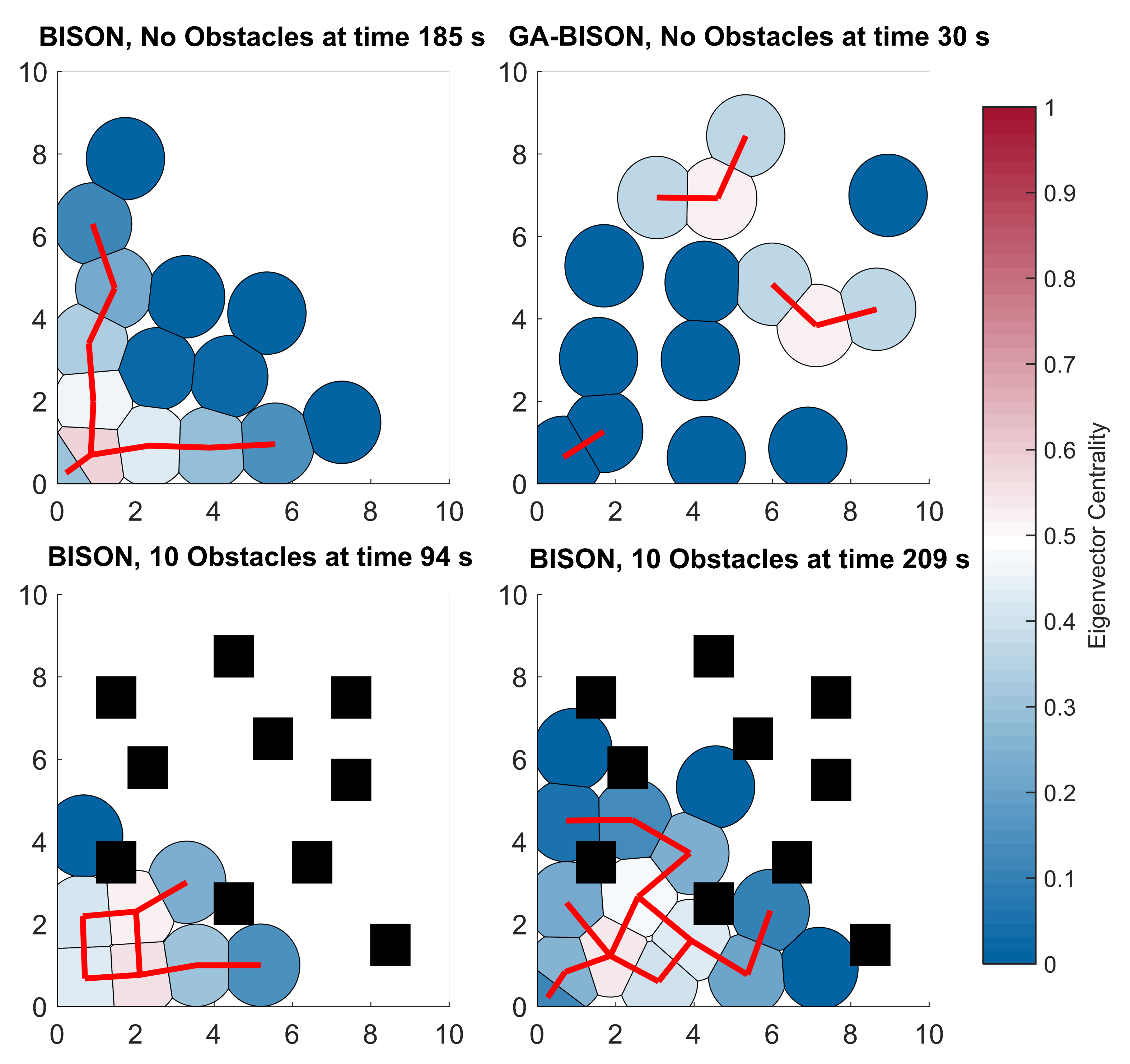
• With Voronoi-only, nodes move outwards during their deployment in a regular fashion, and their importance to connectivity and information relaying drops off with this outward movement. GA + Voronoi demonstrates similar behavior; however, nodes are more likely to reestablish their importance later.
• We see that Voronoi-only in a noise-free environment maintains a small number of long-lasting connections. Adding noise substantially redistributes those connection lengths. By contrast, GA + Voronoi maintains qualitatively similar connection length distributions through a variety of environments, featuring a rapidly changing topology with short, frequent connections between nodes. In all cases, nodes are highly likely to associate only with nodes sharing a similar deployment time
• We see that noise increases the deviation from regularity, smooths out the EC time trace, and impacts the connection length distribution in the Voronoi-only cases. By contrast, noise has a much smaller impact on the same measures applied to the GA + Voronoi cases. This supports previous work that had indicated Voronoi-only changes substantially in the face of noise, while GA + Voronoi is robust to such environmental changes.
• Utilizing temporal network characteristics allows us to measure and observe the behavior of the network as a whole and if individual nodes.
• All this was possible without the explicit use of physical measurements of the nodes’ coverage or their environment. These measures also suggest some kind of deeper functional equivalence between Voronoi-only in noisy environments and GA + Voronoi.

Such quantification measurements may prove useful in further refining our algorithms, by allowing us to fine-tune communication routing protocols, broadcasting strength, and other implementation details based on the expected behavior [86,87].

While mapping these theoretical network measures onto applied performance metrics can perhaps be challenging, we do believe there are some clear points to take note of. When discussing regularity, we noted that regularity difference rose in the noisy Voronoi-only cases and GA + Voronoi cases. This irregularity seems to have some correspondence to speed of coverage, and we posit that such highly irregular structures may be crucial in this rapid deployment. By contrast, the lower regularity difference of Voronoi-only likely corresponds to its slower but more consistent nature. This parallels the behavior we see in measuring percent area covered (PAC), with GA + Voronoi rapidly reaching high levels of PAC, while Voronoi-only slowly converges towards an acceptable value.

We also discussed EC among nodes in the various cases. By looking at EC, we see that nodes consistently move towards positions of lower importance, especially in the Voronoi-only cases. Fluctuations following this are indicative of a node relocating/reorganizing itself in the network and are much more common in the application of GA + Voronoi. This fluctuating corresponds to the cumulative distance traveled (CDT) measures. Assuming a fluctuating EC value corresponds to a particularly mobile node, we would expect the distance travel to be much higher for cases with fluctuating EC. Indeed, our previous research indicated GA + Voronoi nodes travel significantly longer distances, seemingly matching this explanation.

In addition to time evolution of irregularity (Section 6) and time evolution of eigenvector centrality (Section 7), we analyzed the nodes degree distribution, where analogous observations could be made. In the interest of brevity, this output is presented in SOM D, E.

References

1. Holme, P. Modern temporal network theory: A colloquium. Eur. Phys. J. B 2015, 88, 1–30. [Google Scholar] [CrossRef] [Green Version]
2. Li, A.; Cornelius, S.P.; Liu, Y.Y.; Wang, L.; Barabási, A.L. The fundamental advantages of temporal networks. Science 2017, 358, 1042–1046. [Google Scholar] [CrossRef] [PubMed]
3. Michail, O. An Introduction to Temporal Graphs: An Algorithmic Perspective. Internet Math. 2015, 12, 308–343. [Google Scholar]
4. Eledlebi, K.; Hildmann, H.; Ruta, D.; Isakovic, A.F. A Hybrid Voronoi Tessellation/Genetic Algorithm Approach for the Deployment of Drone-Based Nodes of a Self-Organizing Wireless Sensor Network (WSN) in Unknown and GPS Denied Environments. Drones 2020, 4, 33. [Google Scholar] [CrossRef]
5. Eledlebi, K.; Ruta, D.; Hildmann, H.; Saffre, F.; Alhammadi, Y.; Isakovic, A. Coverage and Energy Analysis of Mobile Sensor Nodes in Obstructed Noisy Indoor Environment: A Voronoi-Approach. IEEE Trans. Mob. Comput. 2020. [Google Scholar] [CrossRef]
6. Camazine, S.; Deneubourg, J.; Franks, N.; Sneyd, J.; Theraula, G.; Bonabeau, E. Self-Organization in Biological Systems; Princeton Studies in Complexity, Princeton University Press: Princeton, NJ, USA, 2003. [Google Scholar]
7. Eledlebi, K.; Ruta, D.; Saffre, F.; Al-Hammadi, Y.; Isakovic, A.F. Autonomous Deployment of Mobile Sensors Network in an Unknown Indoor Environment with Obstacles. In Proceedings of the Genetic and Evolutionary Computation Conference Companion, Kyoto, Japan, 15–19 July 2018. [Google Scholar]
8. Eledlebi, K.; Ruta, D.; Saffre, F.; Isakovic, A.F. Self-deployment of Mobile Sensors Network: Indoor Obstacles and Energy Studies. In Proceedings of the 15th IEEE International Conference on Automatic Computing, Trento, Italy, 3–7 September 2018. [Google Scholar]
9. Farine, D.R. When to choose dynamic vs. static social network analysis. J. Anim. Ecol. 2018, 87, 128–138. [Google Scholar] [CrossRef] [Green Version]
10. Wang, G.; Cao, G.; La Porta, T. Movement-assisted sensor deployment. IEEE Trans. Mob. Comput. 2006, 5, 640–652. [Google Scholar] [CrossRef]
11. Zou, J.; Gundry, S.; Kusyk, J.; Sahin, C.S.; Uyar, M.U. Bio-inspired and Voronoi-based Algorithms for Self-positioning of Autonomous Vehicles in Noisy Environments. In Proceedings of the 8th International Conference on Bioinspired Information and Communication Technologies, Boston, MA, USA, 1–3 December 2014. [Google Scholar]
12. Deb, C.; Frei, M.; Schlueter, A. Identifying temporal properties of building components and indoor environment for building performance assessment. Build. Environ. 2020, 168, 106506. [Google Scholar] [CrossRef]
13. Farine, D. The dynamics of transmission and the dynamics of networks. J. Anim. Ecol. 2017, 86, 415–418. [Google Scholar] [CrossRef] [Green Version]
14. Caceres, R.S.; Berger-Wolf, T. Temporal Scale of Dynamic Networks. In Temporal Networks; Springer: Berlin/Heidelberg, Germany, 2013; pp. 65–94. [Google Scholar]
15. Huang, J.L.; Andrello, M.; Martensen, A.C.; Saura, S.; Liu, D.F.; He, J.H.; Fortin, M.J. Importance of spatio-temporal connectivity to maintain species experiencing range shifts. Ecography 2020, 43, 591–603. [Google Scholar] [CrossRef]
16. Wilson, A.; Krause, S.; Ramnarine, I.; Borner, K.; Clément, R.; Kurvers, R.; Krause, J. Social networks in changing environments. Behav. Ecol. Sociobiol. 2015, 69, 1617–1629. [Google Scholar] [CrossRef]
17. Yates, C.A.; Erban, R.; Escudero, C.; Couzin, I.D.; Buhl, J.; Kevrekidis, I.G.; Maini, P.K.; Sumpter, D.J.T. Inherent Noise can Facilitate Coherence in Collective Swarm Motion. Proc. Natl. Acad. Sci. USA 2009, 106, 5464–5469. [Google Scholar] [CrossRef] [Green Version]
18. Ingelrest, F.; Barrenetxea, G.; Schaefer, G.; Vetterli, M.; Couach, O.; Parlange, M. Sensor Scope: Application-specific Sensor Network for Environmental Monitoring. ACM Trans. Sens. Netw. 2010, 6, 1–30. [Google Scholar] [CrossRef]
19. Herrmann, C.; Barthélemy, M.; Provero, P. Connectivity distribution of spatial networks. Phys. Rev. E 2003, 68, 026128. [Google Scholar] [CrossRef] [Green Version]
20. Pan, R.K.; Saramäki, J. Path lengths, correlations, and centrality in temporal networks. Phys. Rev. E 2011, 84, 016105. [Google Scholar] [CrossRef] [Green Version]
21. Presigny, C.; Holme, P.; Barrat, A. Building surrogate temporal network data from observed backbones. Phys. Rev. E 2021, 103, 052304. [Google Scholar] [CrossRef]
22. Aslak, U.; Rosvall, M.; Lehmann, S. Constrained information flows in temporal networks reveal intermittent communities. Phys. Rev. E 2018, 97, 062312. [Google Scholar] [CrossRef] [Green Version]
23. Davidsen, J.; Ebel, H.; Bornholdt, S. Emergence of a Small World from Local Interactions: Modeling Acquaintance Networks. Phys. Rev. Lett. 2002, 88, 128701. [Google Scholar] [CrossRef] [Green Version]
24. Ozik, J.; Hunt, B.; Ott, E. Growing networks with geographical attachment preference: Emergence of small worlds. Phys. Rev. E 2004, 69, 026108. [Google Scholar] [CrossRef]
25. Callaway, D.S.; Hopcroft, J.E.; Kleinberg, J.M.; Newman, M.E.J.; Strogatz, S.H. Are randomly grown graphs really random? Phys. Rev. E 2001, 64, 041902. [Google Scholar] [CrossRef] [Green Version]
26. Gemao, B.; Lai, P.Y. Effects of hidden nodes on noisy network dynamics. Phys. Rev. E 2021, 103, 062302. [Google Scholar] [CrossRef] [PubMed]
27. Blum, C. Ant Colony Optimization: Introduction and Recent Trends; Elsevier: Amsterdam, The Netherlands, 2005; Volume 2, pp. 353–373. [Google Scholar]
28. Liu, X. Sensor Deployment of Wireless Sensor Networks Based on Ant Colony Optimization with Three Classes of Ant Transitions. IEEE Commun. Lett. 2012, 16, 1604–1608. [Google Scholar] [CrossRef]
29. Kulkarni, R.V.; Venayagamoorthy, G.K. Particle Swarm Optimization in Wireless Sensor Networks: A Brief Survey. IEEE Trans. Syst. Man Cybern. 2011, 41, 262–267. [Google Scholar] [CrossRef] [Green Version]
30. Park, H.; Han, J.-H.; Kim, J.-H. Swarm Intelligence-based Sensor Network Deployment Strategy. In Proceedings of the IEEE Congress on Evolutionary Computation, Barcelona, Spain, 18–23 July 2010. [Google Scholar]
31. Zihao, F.; Wei, Z. Network Coverage Optimization Strategy in Wireless Sensor Networks Based on Particle Swarm Optimization; University of Gavle: Gavle, Sweden, 2011. [Google Scholar]
32. Yoon, Y.; Kim, Y.-H. An Efficient Genetic Algorithm for Maximum Coverage Deployment in Wireless Sensor Networks. IEEE Trans. Cybern. 2013, 43, 1473–1483. [Google Scholar] [CrossRef]
33. Trivedi, A.; Srinivasan, D.; Sanyal, K.; Ghosh, A. A Survey of Multiobjective Evolutionary Algorithms Based on Decomposition. IEEE Trans. Evol. Comput. 2017, 21, 440–462. [Google Scholar] [CrossRef]
34. Du, Q.; Faber, V.; Gunzburger, M. Centroidal Voronoi Tessellations: Applications and Algorithms. Soc. Ind. Appl. Math. Rev. 1999, 41, 637–676. [Google Scholar] [CrossRef] [Green Version]
35. Abo-Zahhad, M.; Sabor, N.; Sasaki, S.; Ahmed, S.M. A Centralized Immune-voronoi Deployment Algorithm for Coverage Maximization and Energy Conservation in Mobile Wireless Sensor Networks. Inf. Fusion 2015, 30, 36–51. [Google Scholar] [CrossRef]
36. Pietrabissa, A.; Francesco, L.; Guido, O. A Distributed Algorithm for Ad-hoc Network Partitioning Based on Voronoi Tessellation; Elsevier: Amsterdam, The Netherlands, 2016; Volume 46, pp. 37–47. [Google Scholar]
37. Li, Y.; Dong, T.; Bikdash, M.; Song, Y.-D. Path Planning for Unmanned Vehicles Using Ant Colony Optimization on a Dynamic Voronoi Diagram. IC-AI 2005, 2, 716–721. [Google Scholar]
38. Marbate, P.; Jaini, P. Role of Voronoi Diagram Approach in Path Planning. Int. Eng. Sci. Tech. 2013, 5, 527. [Google Scholar]
39. Kumar, M.; Gupta, V. Benefits of Using Particle Swarm Optimization and Voronoi Diagram for Coverage in Wireless Sensor Networks. In Proceedings of the IEEE International Conference on Emerging Trends in Computing and Communication Technologies (ICETCCT), Dehradun, India, 17–18 November 2017. [Google Scholar]
40. Ab Aziz, N.A.B.; Mohemmed, A.W.; Sagar, B.S.D. Particle Swarm Optimization and Voronoi Diagram for Wireless Sensor Networks Coverage Optimization. In Proceedings of the International Conference on Intelligent and Advanced Systems, Kuala Lumpur, Malaysia, 25–28 November 2007. [Google Scholar]
41. Ab Aziz, N.A.B.; Mohemmed, A.W.; Alias, M.Y. A Wireless Sensor Network Coverage Optimization Algorithm Based on Particle Swarm Optimization and Voronoi Diagram. In Proceedings of the 2009 IEEE International Conference on Networking, Sensing and Control, Okayama, Japan, 26 March 2009. [Google Scholar]
42. Qu, Y.; Georgakopoulos, S.V. A Centralized Algorithm for Prolonging the Lifetime of Wireless Sensor Networks Using Particle Swarm Optimization. In Proceedings of the IEEE Wireless and Microwave Technology Conference (WAMICON 2012 ), Cocoa Beach, FL, USA, 15–17 April 2012. [Google Scholar]
43. Lee, K.-B.; Kim, J.-H. Multi-objective Particle Swarm Optimization with Preference-based Sort and its Application to Path Following Footstep Optimization for Humanoid Robots. IEEE Trans. Evol. Comput. 2013, 17, 755–766. [Google Scholar] [CrossRef]
44. Nematy, F.; Rahmani, N. Using Voronoi Diagram and Genetic Algorithm to Deploy Nodes in Wireless Sensor Network. Int. J. Soft Comput. Softw. Eng. 2013, 3, 706–713. [Google Scholar]
45. Rahmani, N.; Nematy, F.; Rahmani, A.M.; Hosseinzadeh, M. Node Placement for Maximum Coverage Based on Voronoi Diagram Using Genetic Algorithm in Wireless Sensor Networks. Aust. J. Basic Appl. Sci. 2011, 5, 3221–3232. [Google Scholar]
46. Banimelhem, O.; Mowafi, M.; Aljoby, W. Genetic Algorithm Based Node Deployment in Hybrid Wireless Sensor Network. Commun. Netw. 2013, 5, 273–279. [Google Scholar] [CrossRef] [Green Version]
47. Jia, J.; Chen, J.; Chang, G.; Li, J.; Jia, Y. Coverage Optimization based on Improved NSGA-II in Wireless Sensor Network. In Proceedings of the IEEE International Conference on Integration Technology, Shenzhen, China, 20–24 March 2007. [Google Scholar]
48. Zou, J.; Kusyk, J.; Uyar, M.Ü.; Gundry, S.; Sahin, C.S. Bio-inspired and Voronoi-based Algorithms for Self-positioning Autonomous Mobile Nodes. In Proceedings of the MILCOM 2012—IEEE Military Communications Conference, Orlando, FL, USA, 29 October–1 November 2012. [Google Scholar]
49. Fister, I.; Mernik, M.; Brest, J. Hybridization of evolutionary algorithms. arXiv 2013, arXiv:1301.0929. [Google Scholar]
50. Cortes, J.; Martinez, S.; Karatas, T.; Bullo, F. Coverage Control for Mobile Sensing Networks. IEEE Trans. Robot. 2004, 20, 243–255. [Google Scholar] [CrossRef]
51. Qu, Y.; Georgakopoulos, S.V. Relocation of Wireless Sensor Network Nodes using a Genetic Algorithm. In Proceedings of the 12th Annual IEEE Wireless and Microwave Technology Conference (WAMICON), Clearwater Beach, FL, USA, 18–19 April 2011; pp. 1–5. [Google Scholar]
52. Bhondekar, A.P.; Renu, V.; Singla, M.; Ghanshyam, G. Genetic Algorithm Based Node Placement Methodology for Wireless Sensor Networks. In Proceedings of the International MultiConference of Engineers and Computer Scientists, Hong Kong, 18–20 March 2009. [Google Scholar]
53. Kaur, S.; Uppal, R.S. Dynamic deployment of homogeneous sensor nodes using genetic algorithm with maximum coverage. In Proceedings of the 2015 2nd International Conference on Computing for Sustainable Global Development (INDIACom), New Delhi, India, 11–13 March 2015; pp. 470–475. [Google Scholar]
54. Norouzi, A.; Zaim, A.H. Genetic Algorithm Application in Optimization of Wireless Sensor Networks. Sci. World J. 2014, 14, 1–15. [Google Scholar] [CrossRef]
55. Hosseinirad, S.M.; Basu, S.K. Wireless Sensor Network Design Through Genetic Algorithm. J. Data Mining 2014, 2, 85–96. [Google Scholar]
56. Romoozi, M.; Vahidipour, M.; Romoozi, M.; Maghsoodi, S. Genetic Algorithm for Energy Efficient and Coverage-preserved Positioning. In Proceedings of the IEEE International Conference on Intelligent Computing and Cognitive Informatics, Kuala Lumpur, Malaysia, 22–23 June 2010. [Google Scholar]
57. Tahir, N.N.M.; Atan, F. A Modified Genetic Algorithm Method for Maximum Coverage in Dynamic Mobile Wireless Sensor Networks. J. Basic Appl. Sci. Res. 2016, 6, 26–32. [Google Scholar]
58. Hassan, R.; Cohanim, B.; De Weck, O.; Venter, G. A Comparison of Particle Swarm Optimization and The Genetic Algorithm. In Proceedings of the 46th AIAA/ASME/ASCE/AHS/ASC Structures, Structural Dynamics and Materials Conference, Austin, TX, USA, 18–21 April 2005. [Google Scholar]
59. Friedrich, T.; Kotzing, T.; Krejca, M.S. The Compact Genetic Algorithm is Efficient Under Extreme Gaussian Noise. IEEE Trans. Evol. Comput. 2017, 21, 477–490. [Google Scholar] [CrossRef]
60. Zhang, Y.; Gong, Y.; Gao, Y.; Wang, H.; Zhang, J. Parameter-Free Voronoi Neighborhood for Evolutionary Multimodal Optimization. IEEE Trans. Evol. Comput. 2020, 24, 335–349. [Google Scholar] [CrossRef]
61. Kramer, O. Genetic Algorithm Essentials; Studies in Computational Intelligence; Springer International Publishing: Berlin/Heidelberg, Germany, 2017. [Google Scholar]
62. Bhondekar, A.; Renu, V.; Singla, M.; Ghanshyam, C.; Pawan, K. Genetic Algorithm Based Node Placement Methodology for Wireless Sensor Networks. Lect. Notes Eng. Comput. Sci. 2009, 2174, 18–20. [Google Scholar]
63. Holme, P.; Saramäki, J. Temporal Networks; Understanding Complex Systems; Springer: Berlin/Heidelberg, Germany, 2013. [Google Scholar]
64. He, M.; Pathak, S.; Muaz, U.; Zhou, J.; Saini, S.; Malinchik, S.; Sobolevsky, S. Pattern and Anomaly Detection in Urban Temporal Networks. arXiv 2019, arXiv:1912.01960. [Google Scholar]
65. Antulov-Fantulin, N.; Lancic, A.; Smuc, T.; Stefancic, H.; Sikic, M. Identification of Patient Zero in Static and Temporal Networks: Robustness and Limitations. Phys. Rev. Lett. 2015, 114, 248701. [Google Scholar] [CrossRef] [Green Version]
66. Caballero, J.; Ledig, C.; Aitken, A.; Acosta, A.; Totz, J.; Wang, Z.; Shi, W. Real-Time Video Super-Resolution with Spatio-Temporal Networks and Motion Compensation. In Proceedings of the 2017 IEEE Conference on Computer Vision and Pattern Recognition (CVPR), Honolulu, HI, USA, 21–26 July 2017; pp. 2848–2857. [Google Scholar]
67. Venkatesh, P.; Prakash, G.C. Centrality Measures To Ascertain Leaders In Wireless Sensor Networks. J. Emerg. Technol. Innov. Res. 2019, 6, 12–16. [Google Scholar]
68. Jain, A.; Reddy, B. Node centrality in wireless sensor networks: Importance, applications and advances. In Proceedings of the 2013 3rd IEEE International Advance Computing Conference (IACC), Ghaziabad, India, 22–23 February 2013; pp. 127–131. [Google Scholar]
69. Santoro, N.; Quattrociocchi, W.; Flocchini, P.; Casteigts, A.; Amblard, F. Time-Varying Graphs and Social Network Analysis: Temporal Indicators and Metrics. arXiv 2011, arXiv:1102.0629. [Google Scholar]
70. Ducrocq, T.; Hauspie, M.; Mitton, N.; Pizzi, S. On the Impact of Network Topology on Wireless Sensor Networks Performances: Illustration with Geographic Routing. In Proceedings of the 2014 28th International Conference on Advanced Information Networking and Applications Workshops, Victoria, BC, Canada, 13–16 May 2014; pp. 719–724. [Google Scholar]
71. Weng, T.; Zhang, J.; Small, M.; Zheng, R.; Hui, P. Memory and betweenness preference in temporal networks induced from time series. Sci. Rep. 2017, 7, 41951. [Google Scholar] [CrossRef] [Green Version]
72. Kivelä, M.; Cambe, J.; Saramäki, J.; Karsai, M. Mapping temporal-network percolation to weighted, static event graphs. Sci. Rep. 2018, 8, 12357. [Google Scholar] [CrossRef]
73. Taylor, D.; Porter, M.; Mucha, P. Tunable Eigenvector-Based Centralities for Multiplex and Temporal Networks. Multiscale Model. Simul. 2021, 19, 113–147. [Google Scholar] [CrossRef]
74. Al Mugahwi, M.; De La Cruz Cabrera, O.; Fenu, C.; Reichel, L.; Rodriguez, G. Block matrix models for dynamic networks. Appl. Math. Comput. 2021, 402, 126121. [Google Scholar] [CrossRef]
75. Radicchi, F.; Arenas, A. Abrupt transition in the structural formation of interconnected networks. Nat. Phys. 2013, 9, 717–720. [Google Scholar] [CrossRef] [Green Version]
76. Estrada, E. The Structure of Complex Networks: Theory and Applications; Oxford University Press: Oxford, UK, 2011. [Google Scholar]
77. Abbasi, M.A. Realization of centrality measure on Wireless Sensor Network. In Proceedings of the 2017 International Conference on Innovations in Electrical Engineering and Computational Technologies (ICIEECT), Karachi, Pakistan, 5–7 April 2017; pp. 1–6. [Google Scholar]
78. Kumaran, R.S.; Suganya, P. Network Lifetime Enhancement in Wireless Sensor Networks Using Energy Aware Clustering with Fuzzy System. J. Phys. Conf. Ser. 2021, 1717, 012069. [Google Scholar] [CrossRef]
79. Ahmad, T.; Li, X.J.; Seet, B.C.; Cano, J.C. Social Network Analysis Based Localization Technique with Clustered Closeness Centrality for 3D Wireless Sensor Networks. Electronics 2020, 9, 738. [Google Scholar] [CrossRef]
80. Borgatti, S.P.; Carley, K.M.; Krackhardt, D. On the robustness of centrality measures under conditions of imperfect data. Soc. Netw. 2006, 28, 124–136. [Google Scholar] [CrossRef] [Green Version]
81. Labatut, V.; Ozgovde, A. Topological Measures for the Analysis of Wireless Sensor Networks. Procedia Comput. Sci. 2012, 10, 397–404. [Google Scholar] [CrossRef]
82. Jacoby, D.M.; Freeman, R. Emerging Network-Based Tools in Movement Ecology. Trends Ecol. Evol. 2016, 31, 301–314. [Google Scholar] [CrossRef] [PubMed]
83. Orman, G.K.; Labatut, V.; Naskali, A.T. Exploring the Evolution of Node Neighborhoods in Dynamic Networks. Phys. Stat. Mech. Its Appl. 2017, 482, 375–391. [Google Scholar] [CrossRef] [Green Version]
84. Dablander, F.; Hinne, M. Node centrality measures are a poor substitute for causal inference. Sci. Rep. 2019, 9, 6846. [Google Scholar] [CrossRef] [PubMed] [Green Version]
85. Sneppen, K. Models of Life: Dynamics and Regulation in Biological Systems; Cambridge University Press: Cambridge, UK, 2014. [Google Scholar] [CrossRef]
86. Maraiya, K.; Kant, K.; Gupta, N. Application based Study on Wireless Sensor Network. Int. J. Comp. Appl. 2011, 21, 9–15. [Google Scholar] [CrossRef]
87. Ko, J.; Lim, J.H.; Chen, Y.; Musvaloiu-E, R.; Terzis, A.; Masson, G.M.; Gao, T.; Destler, W.; Selavo, L.; Dutton, R.P. Medical Emergency Detection in Sensor Networks. ACM Trans. Embed. Comput. Syst. 2010, 10, 361–362. [Google Scholar] [CrossRef]
Figure 1. Illustration of the evolution of nodes using Voronoi-only and Ga + Voronoi algorithms. The red lines indicate a suitable network connection for information routing. Nodes are colored based on their eigenvector centrality (cf. Section 7). Additional materials offered in SOM-B.
Applsci 12 01315 g001
Figure 2. Snapshots of a WSN generated by (upper) the Voronoi-only algorithm and (lower) the GA-BISON algorithm in an obstacle-free environment, at different time steps. ND signifies noise level (chosen from 0.01 , 0.05 , 0.1 ). See Equation (2).
Applsci 12 01315 g002
Figure 3. Edge-centric representation of Voronoi-only (BISON) and GA + Voronoi (GA-BISON) in both the obstacle-free environment and obstacle-rich environments. A given simulation has reached the cut-off condition at its rightmost edge. Notice that GA + Voronoi reaches cutoff after a fraction of the time required for Voronoi-only, and how Voronoi-only performs much more quickly in the presence of noise. Furthermore, note the sporadic nature of connections within GA + Voronoi, compared to the stability of Voronoi-only connections. (a,b) Two of the significant empty bands, where connections never form. Table 3 on the next page lists the connections in panels (a,b), we refer to SOM-C for a complete list of all missing pairs, for all panels of this figure.
Applsci 12 01315 g003
Figure 4. Distribution of various lengths of connection for each of the cases in Figure 3. We see a drastic qualitative difference between Voronoi-only in noise-free and noisy environments, and smaller quantitative difference between GA + Voronoi cases.
Applsci 12 01315 g004
Figure 5. Temporal evolution of the deviation from regularity for Voronoi-only and GA + Voronoi approaches under different environmental conditions. We note the need to use log scale for the time axis indicating an order of magnitude difference between the characteristic time scale for two methods. The measure Δ reg is defined in Equation (4), above. (a) Comparison of BISON only and GA+BISON performance with varied noise but without scaterrers. (b) Comparison of BISON only and GA+BISON performance with varied noise, and in the presence of scaterrers.
Applsci 12 01315 g005
Figure 6. Eigenvector Centralities of the Voronoi-only approach in various environments at different time steps; Vertical bar sign “ 0.6 ”, stacked vertically, is common to all curves.
Applsci 12 01315 g006
Figure 7. Eigenvector Centralities of GA + Voronoi in various environments at different time steps; Vertical bar sign “ 0.6 ” is common to all curves, which are stacked vertically for clarity.
Applsci 12 01315 g007
Figure 8. Time -lag correlation heat maps for time-dependent eigenvector centralities from Figure 6 and Figure 7. (selected node pairs shown only—more data in SOM). (upper) Voronoi; (lower) GA + Voronoi; (both) ND = 0.05 and 10 obstacles.
Applsci 12 01315 g008