Abstract
A smoothing localization method for Global Navigation Satellite System (GNSS) and visual Simultaneous Localization and Mapping (SLAM) system is proposed to identify GNSS spoofing, optimize the cumulative error of the GNSS/visual SLAM system, and obtain smoothing localization results. The proposed method analyzes the joint error distribution of the GNSS/visual SLAM system, uses the visual frame to invert the relative error offset of the GNSS from the dimensions of time and localization, performs error analysis and mutual verification based on the verification threshold. According to the mutual verification results, the GNSS spoofing is identified, and the corresponding back-end optimization strategy is selected to obtain a smoothing localization result. Through simulation, the time verification threshold and localization verification threshold of the proposed method are obtained under the condition that the sensors frequency and accuracy are set. The KITTI datasets in rural and urban scenes are used for verification. The simulation results show that our method can identify GNSS spoofing and provide credible and smoothing localization results in the case of GNSS spoofing occurs.
1. Introduction
Localization is the most basic and important part for mobile terminals in autonomous driving, robots, and Internet of Vehicles. Currently, navigation and positioning systems based on GNSS are the most widely used. GNSS is the only method that can provide global absolute position coordinates. However, its signals are publicly available, which makes its localization easy to be spoofed. In recent years, with the improvement of mobile terminal computing performance, the use of camera sensors to obtain visual SLAM data has been widely used [1]. The visual mileage information provided by SLAM can simultaneously match the observed environmental features with the feature map to obtain pose and autonomous localization [2]. However, the visual SLAM method can only provide the relative pose of the mobile terminal, and cannot provide the global localization coordinates, such as VINS-Mono [3], ORB-SLAM1-3 [4,5,6].
In outdoor scenes, GNSS is still indispensable. In general, visual SLAM sensors use GNSS to provide localization for initialization and global pose calibration, such as VINS-Fusion [7] and GVINS [8]. The fusion of visual SLAM system and GNSS system can make up for the limitations of SLAM relative localization, so that the mobile terminal can obtain global localization information, realize positioning globalization and higher-precision localization results. Although system fusion improves positioning accuracy, it also brings new problems. GNSS signals are public and vulnerable to spoofing attacks. Once a GNSS spoofing attack occurs, the result of system fusion positioning will become unreliable, reducing the security of the mobile terminal during the movement [9].
A general optimization framework that supports multi-sensor mileage estimation such as GPS and VINS is proposed in reference [7], and the performance of the system is verified in public data sets and through multi-sensor actual experiments. However, this reference focuses on the optimization of the framework algorithm without considering the possible impact of GNSS spoofing. GVINS can make up for the lack of GNSS by obtaining tightly coupled results through camera, IMU and GNSS [8]. In order to suppress unstable satellite signals, only satellites that have been locked for a period of time are allowed to enter the system for optimization, but this method also does not consider the possible occurrence of GNSS spoofing. If malicious GNSS spoofing attack occurs, deviation errors will be injected into the localization calculation process, causing the GNSS localization result to deviate from the correct position [10]. For the mobile terminal, the deviation errors of the localization result will cause it to move to a pre-set location by the fraudster, and thus be kidnapped [11,12].
Some researchers have done research on the problem of unreliable GNSS data caused by GNSS spoofing. Reference [13] proposes a RIO method to judge whether the positioning solution meets the distance constraint based on the information of the GNSS/IMU/ODOM system to counter GNSS spoofing attack. Reference [14] reconstructed the distribution of spoofing signals in the signal domain, and proposed a MEMS-INS/GNSS tightly coupled spoofing identification method based on spoofing contour estimation to identify and eliminate GNSS spoofing attacks. Reference [15] proposed a credible Kalman filter algorithm model to identify GNSS attacks through auxiliary sensor systems to obtain credible navigation results. These methods used traditional navigation sensors (GNSS, inertial measurement unit, and odometer) without considering the possibility of visual SLAM system in GNSS spoofing identification.
In order to better identify the GNSS spoofing using visual SLAM system and improve the localization accuracy of the system, we combine the data of GNSS with the visual SLAM system to identify GNSS spoofing attacks and obtain global smoothing localization results. This method uses the time stamp and relative pose information obtained by the visual SLAM system to perform error inversion on the GNSS data, and conduct mutual verification between the GNSS and the visual SLAM system. In this way, GNSS spoofing can be identified, the cumulative error of vision SLAM system can be optimized, and the smoothing localization result can be obtained to resist the possible risk of GNSS spoofing. Finally, the method is verified in different scenes of the KITTI dataset. The simulation results show that our method can eliminate GNSS spoofing and provide relatively reliable and smoothing localization results for mobile terminals.
2. System Model
2.1. Model Description
The GNSS spoofing identification and smoothing localization model is divided into front-end and back-end. The front-end refers to the acquisition of data from each sensor and modeling, and the back-end refers to the processing of the data from each sensor. At the front-end of the system, the measurement inputs of GNSS and visual SLAM system are processed separately. First, model the acquired GNSS measurement data, perform pseudorange calculation and coordinate conversion, and initialize the absolute coordinate of the system. Then, model the acquired visual SLAM measurement data and perform pose calculation and optimizing. At the back-end of the system, use the time and pose information of visual SLAM system to invert the relative time error and localization offset of GNSS data, and perform time and localization verification on GNSS measurement data to analyze whether GNSS spoofing has occurred. The GNSS data frames that if time-localization verification passes, it will be input into the back-end optimization process to optimize the cumulative error of the visual SLAM, and the GNSS data frames that have not passed the time-localization verification will be discarded. Finally, two strategies of the GNSS/Visual SLAM back-end smoothing localization method are selected according to the results of the time and localization verification to perform smoothing localization results.
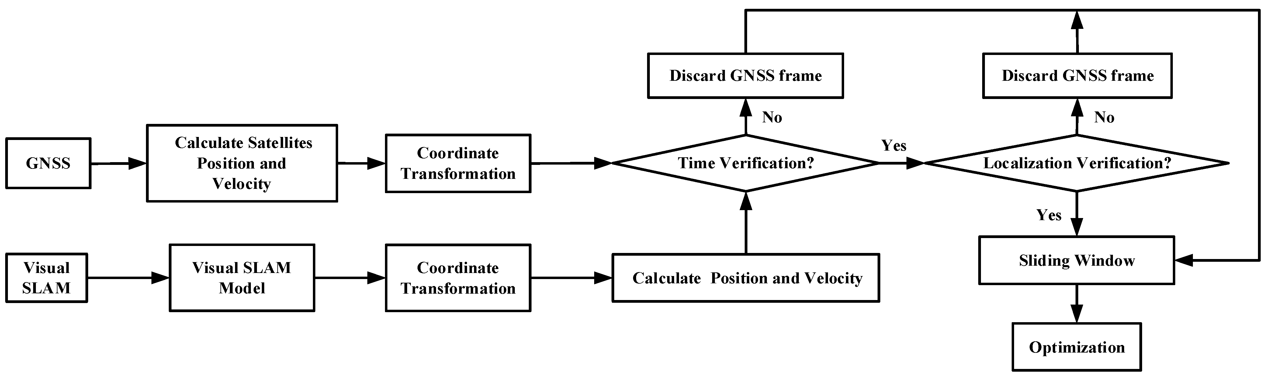
The following of this section is the modeling and error analysis of the measurement data of the GNSS and visual SLAM system. In Section 3, the time-localization mutual verification, localization verification threshold and smoothing localization method are analyzed. In Section 4, Section 5 and Section 6, parameter analysis and experiment simulation are carried out. The GNSS spoofing identification and smoothing localization model is shown in Figure 1.
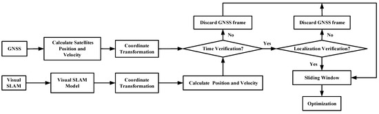
Figure 1.
GNSS spoofing identification and smoothing localization model.
2.2. GNSS Coordinate Calculation and Conversion
The coordinate calculation of GNSS receiver is based on the information of four or more satellites received by the GNSS receiver. There are two steps. First, calculate the pseudorange of the GNSS receiver based on the received information, and then calculate the localization coordinates of the GNSS receiver based on the pseudorange.
The pseudorange is calculated based on the distance between the satellite and the GNSS receiver, taking into account the errors of ionosphere and troposphere. Assuming that the receiver localization coordinate is , the satellite coordinate obtained by the receiver through the analysis of the received satellite signals is , where n represents the satellite number, represents the pseudorange correction value of the nth satellite, represents the clock error between the receiver and the satellite under the coordinates . In addition to the clock error generated by the propagation geometric distance, the clock error also includes the satellite clock error , ionospheric delay , and tropospheric delay , thus
In addition, the receiver will generate measurement noise during the measurement process. Then, the pseudorange solved by the GNSS receiver is
where c is the velocity of light.
The satellite clock error, ionospheric delay and tropospheric delay can all be calculated, which can be regarded as known quantities. The measurement noise generated by the receiver is related to the performance of the receiver itself.
Generally, the possibility that the GNSS localization result exceeds the range is only 0.27% according to the Pauta criterion ( criterion). Thus, an error of can be used as the limit error of the GNSS localization result.
According to the pseudorange positioning equation [16], the localization coordinate and clock error of the receiver can be obtained, which is the localization coordinates of the receiver in the Earth Centered Inertial Coordinate System (ECI). Then, after the receiver’s position calculation, the ECI coordinate is converted to the Longitude Latitude Altitude coordinate system (LLA) to obtain the receiver’s current longitude, latitude and altitude , which is the absolute localization of the mobile terminal in the world coordinate system.
The results of the GNSS position calculation will provide the absolute position information of the mobile terminal in the initialization of the system, and perform mutual verification and smoothing localization with the visual SLAM system in the back-end of the system.
2.3. Visual SLAM System Modeling and Error Analysis
The sensor used in our visual SLAM system is a binocular vision mileage camera. Its localization principle is to estimate the rotation and translation matrix of the camera through the matching relationship between the feature points observed in two adjacent pictures, and to calculate the relative motion path of the camera. For visual SLAM, the relative motion path of the camera is estimated based on the information of two adjacent frames, and there is also an estimation error at time t. With continuous calculations, these errors will gradually accumulate in the positioning results through calculations. If the positioning result is not corrected in time, the positioning error will continue to accumulate and increase, making the posture estimation deviation larger and larger. Therefore, we need to optimize to reduce the accumulation of errors. However, if all the observed frames are optimized to reduce the accumulation of errors, the amount of data will continue to increase. The computational burden to solve the optimization problem will also increase rapidly as the amount of data increases. Therefore, we set a visual processing sliding window (the size of the window is set to m) to store, optimize, and update the key frames constantly to reduce the computational burden of the system, reduce estimation errors, and improve positioning accuracy.
The visual frame optimization algorithm is as follows. First of all, after obtaining the original information of the left-eye and right-eye image of the binocular camera in current frame, the current left-eye image is tracked with the left-eye image of the previous frame using the pyramid LK optical flow method [17] based on corner point features. The matched points between the two frames are retained as feature points, and the points with large differences are eliminated. Then, the feature point set is obtained, defined as . For the right-eye image of the current frame, match it with the left-eye image of the current frame and extract feature points using the same method as above.
Next, determine whether the current frame is a key frame according to the obtained feature point information and update the key frame in the visual processing sliding window. Calculate the number of common-view feature points between the left eye frame and the last key frame in the visual processing sliding window. If the number of common-view feature points is less than the feature point threshold , delete the first frame in the visual processing sliding window, add the current left eye image to the visual processing sliding window as a key frame and sequentially update the key frames in the window (for example, frame is updated to be frame , and frame is updated to be ). Conversely, if the number of common-view feature points is greater than the feature point threshold , delete the last key frame and add the current left-eye image to the visual processing sliding window as a key frame to replace the last frame . Similarly, calculate the number of common-view feature points between the right-eye frame and the last key frame in the window, and update the key frame in the visual processing sliding window.
Then, optimize the feature information of the key frames in the visual processing sliding window and the rotation and translation matrix between frames to update the pose of the camera. The camera pose update is divided into two stages: the initialization stage and the stable updating stage.
In the camera initialization stage, the world 3D coordinates of the feature points observed by the camera are unknown. Assuming that the set of common-view feature points of and is , the normalized camera coordinates of the feature points in the left and right images are and . Then, according to the epipolar constraint [18], the eight-point method [19] and the SVD decomposition method [20], the homogeneous coordinates of feature point in the world 3D coordinate, the depth values and of the feature point in the left and right images and the relative pose of the two frames at this time can be obtained. Similarly, all the world 3D coordinates of feature points can be estimated.
In the stable updating stage, we first use the world 3D coordinates of the common view feature points, the normalized coordinates in the camera frame and depth in the current frame , to calculate the rotation and translation matrix . Then, we use the obtained rotation and translation matrix to estimate the world 3D coordinates of the non-common view feature points. We can get the world 3D coordinates of all feature points in the current frame , and the rotation and translation matrix of the camera in the current frame.
In order to reduce the accumulated mileage error caused by the estimation above, we optimize the depth of the common view feature points of the key frame and the camera pose in the visual processing sliding window. The state vector to be optimized includes the poses of m cameras and the depths of n feature points in the visual processing sliding window, as shown in the following formula:
where is the camera homogeneous transformation matrix containing the rotation and translation matrix information, and is the depth of the feature point observed in the first frame. Then, the visual reprojection error of the feature points from frame to frame is
where is the normalized camera coordinate of feature point in the frame , is the normalized camera coordinate of the feature point observed by the camera for the first time, is the homogeneous transformation matrix from frame to the world coordinate system and is the homogeneous transformation matrix from the world coordinate system to frame . The objective function for optimizing the depth of feature points in the visual processing sliding window and the rotation and translation matrix of the camera is
Through the Ceres solver [21], a stable solution and the optimized of the camera in each frame can be obtained. In the back-end of the system, we can use the optimized of the camera to perform mutual verification with the results of the GNSS position calculation. Let the ENU coordinate vector of the visual SLAM system at time i be defined as . Then, the formula for calculating the motion position of visual SLAM from time i−1 to time i is
3. Time-Localization Verification and Smoothing Localization Method
In the back-end of the system, the time verification and localization verification of GNSS/Visual SLAM are first performed respectively to identify GNSS spoofing. Then, the smoothing localization method is performed to optimize the cumulative error of the localization results.
3.1. Time Verification
Time verification is primarily used to identify whether the GNSS data frames and visual SLAM data frames are synchronized in time. For the original data of the vision system and the GNSS system, there is a certain time deviation between the two data streams, so, time synchronization is required. The ideal method for clock synchronization between different systems is hardware trigger synchronization, but this method requires a high degree of hardware integration, which is difficult to achieve. Therefore, the more common method in engineering is soft synchronization. That is, when data is obtained by the terminal, the system software time stamp is added to the data frame, and time synchronization is performed according to the software time stamp.
In addition, when sensor trigger delay, transmission delay or GNSS spoofing occurs, it may cause a small time misalignment between GNSS and visual SLAM system. So, in time verification process, it is first required to obtain the frame rate of GNSS and visual SLAM data acquisition, and use the sensor with the high frame rate as the reference sensor to perform time verification on the other sensor. In general, although the GNSS system can provide absolute position, its update rate is low, while the visual update rate is high. That is, between two GNSS data frames, there will be many visual frames generated. If the GNSS frame is used as the reference, only the visual frame synchronized with the GNSS will be retained, and other visual data frames will be discarded. In order to be able to retain more frames, we choose the faster sensor (Visual SLAM) as the reference source.
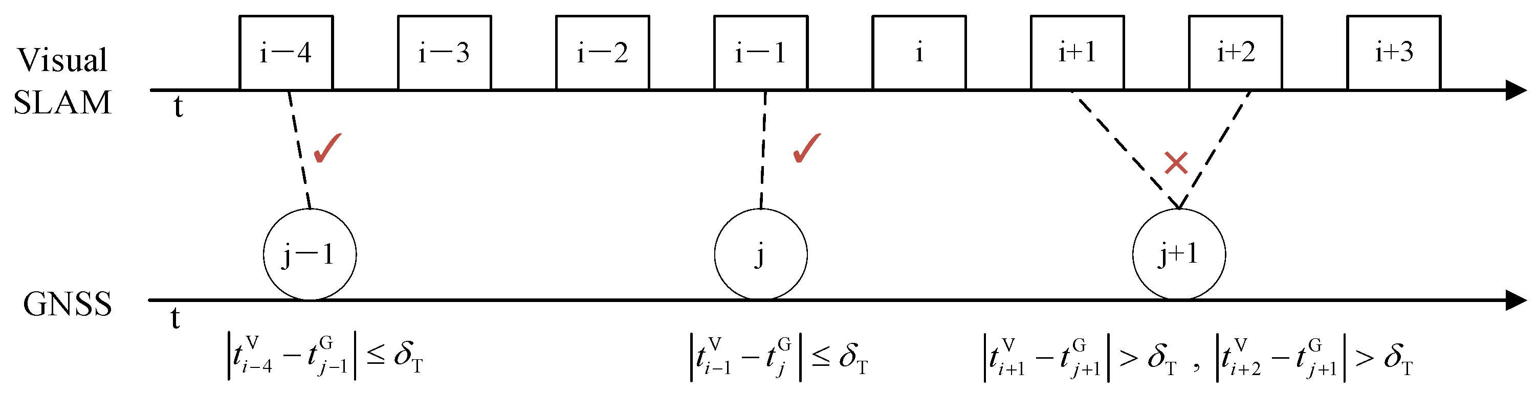
The time deviation between GNSS and visual SLAM system at time i is
where is the timestamp of the visual SLAM system and is the timestamp of the GNSS system.
Let be the time verification threshold of visual SLAM and GNSS data frames (which need to be adjusted according to the actual frame rate of the sensors, for example, 0.01s). In the time verification process, the visual SLAM data frame is set as the main frame, and the GNSS data frame in the buffer is verified according to Equation (15). If , the time deviation between GNSS and visual SLAM system is within the time verification threshold , and the time verification is judged to be normal, and the time domain verification flag is set to ; if , the time deviation between GNSS and visual SLAM system exceeds the threshold range, it is judged that the time domain verification is abnormal, and the time domain verification flag is set to , that is
Localization verification will be processed only after the GNSS frames and the visual SLAM frame are synchronized. If is too large, there are many GNSS frames that meet the threshold, and GNSS data frames that are misaligned with the visual SLAM data frames may be input into the back-end processing, resulting in large spatial errors between the GNSS and visual SLAM data frames, and if is too small, there are fewer GNSS frames that meet the threshold requirement, which will cause normal GNSS data frames to be discarded, and the system will increase the accumulated error due to the lack of GNSS frame calibration. Therefore, the selection of the time verification threshold is very important, and we will conduct simulation analysis in Section 4. The time verification is shown in Figure 2.
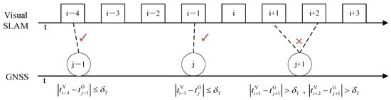
Figure 2.
Time Verification.
After time verification, the GNSS data frame and the visual SLAM data frame are synchronized in time. Next, the visual SLAM data frame and the verified GNSS data frame are input into the localization verification process.
3.2. Localization Verification
In the localization verification process, we need to unify the localization information output by GNSS and visual SLAM system under the same coordinate system. Through the analysis of the visual SLAM frame, the GNSS localization result is inverted to identify whether the GNSS is spoofed.
For the GNSS system, the latitude and longitude coordinates obtained from the GNSS system are first converted to the Earth-centered and Earth-Fixed Coordinate System (ECEF), and then converted to the local Cartesian coordinates coordinate system (ENU) to get to realize the unification of the global coordinate system and the local coordinate system [15]. is the ENU coordinate vector calculated by GNSS system. The origin of the ENU coordinate system is the initial point in the ECEF coordinate system, which is also the initial position of the visual SLAM system.
For the visual SLAM system, we set the left-eye camera as the origin of the camera coordinate system. According to Section 2.3, the ENU coordinate vector of the visual SLAM system at time i is defined as . However, the visual SLAM system is usually not in the same plane with GNSS system, which requires a 4-degree-of-freedom (4DoF) rotation and translation to achieve spatial unification with GNSS. The coordinate conversion relationship between the visual SLAM system and the GNSS system is
where is the external parameters of the camera (It should be noted that is the rotation and translation matrix between the visual frame and the GNSS frame, and is the rotation and translation matrix for visual SLAM system from frame k − 1 to frame k.).
The optimized coordinates of the visual SLAM system in the ENU coordinate system can be obtained as
There are generally two types of GNSS spoofing. One of them is forwarding spoofing. After the forwarding spoofing is tracked to the receiver signal, the location spoofing information is applied, so that the terminal calculates the wrong position and continues to move toward the target point. In fact, it reaches the location designated by the spoofing terminal. The other type is inducing spoofing, which applies small displacement spoofing to the terminal, causing the terminal to be gradually pulled away. Assume that is the location verification threshold of forwarding spoofing and is the location verification threshold of inducing spoofing. The localization verification methods of the two types of spoofing are analyzed separately.
In order to identify whether the GNSS is spoofed, the GNSS measurement data will be checked with visual SLAM data. By inverting the offset of GNSS data, it is judged whether the offset result exceeds the threshold.
When GNSS forwarding spoofing occurs, the forwarding spoofing deviation at time i is
If , the deviation between GNSS and visual SLAM system is within the threshold range, the localization verification is judged to be normal, and the localization domain verification flag is set to . If , the deviation between GNSS and visual SLAM system exceeds the threshold range, the localization verification is judged to be abnormal, and the localization domain verification flag is set to , that is
When GNSS inducing spoofing occurs, since the small drift (usually less than the positioning accuracy of GNSS) applied by spoofing terminal is not easy to be found at each moment, it is necessary to observe the cumulative error within a certain time window.
Suppose the size of the time window is W, then the total spoofing deviation in the time window at time is
If , the deviation between GNSS and visual SLAM system is within the threshold range, the localization verification is judged to be normal, and the localization domain verification flag is set to . If , the deviation between GNSS and visual SLAM system exceeds the threshold range, the localization verification is judged to be abnormal, and the localization domain verification flag is set to . Therefore, regardless of whether forward spoofing or progressive spoofing occurs, GNSS frames need to be discarded. Then, the localization domain verification flag needs to meet
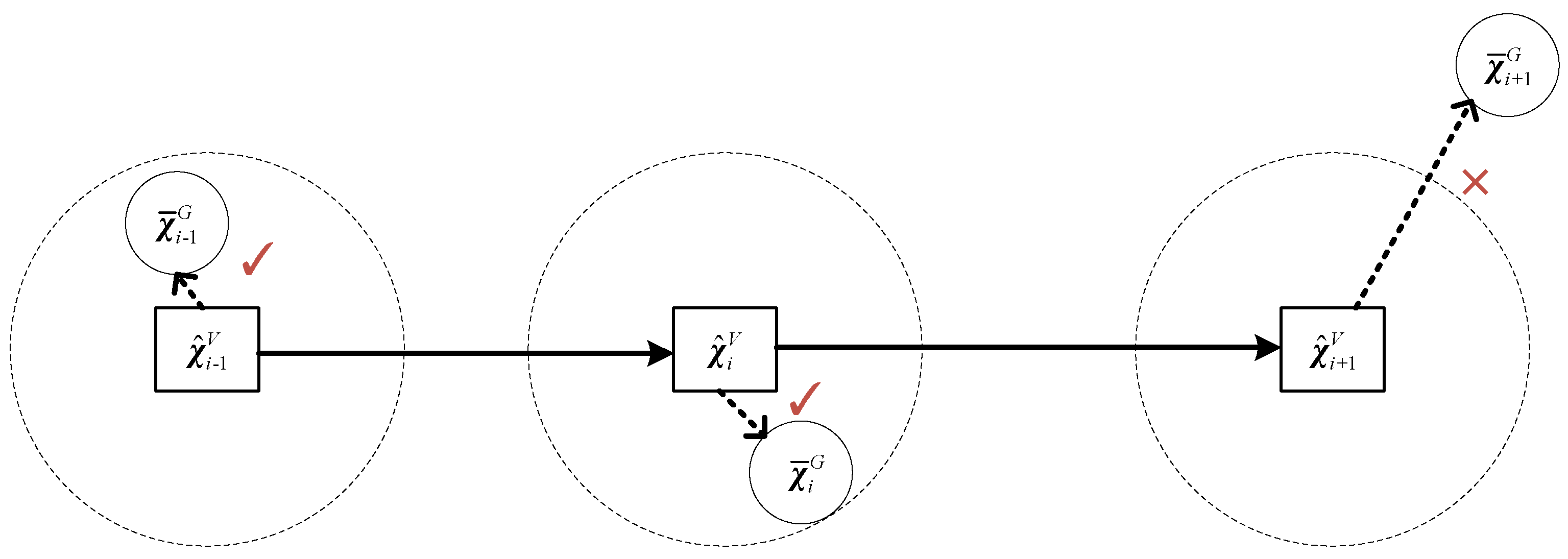
The localization verification is shown in Figure 3. Only the GNSS frames that are verified with the visual SLAM frame will enter the smoothing localization process. If location verification threshold is too large, spoofed GNSS frames that meet the threshold may be input into the smoothing localization process, resulting in localization errors in the back-end of the system, and if location verification threshold is too small, normal GNSS data frames will be discarded. Therefore, the selection of the localization verification threshold is also important. So, we conduct localization verification threshold analysis in Section 3.3. After time and localization verification, the verified GNSS data frames will be input into the smoothing localization process. Then, the system enters the smoothing localization method.
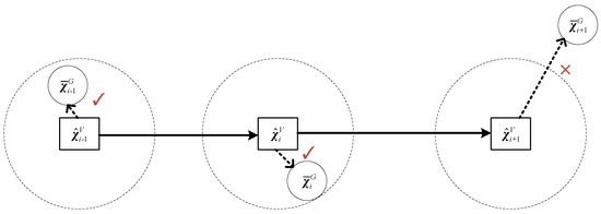
Figure 3.
Localization Verification.
3.3. Localization Verification Threshold Analysis
When the terminal is moving, the position calculated by GNSS is usually within a certain error range from the true value, and the position calculated by the visual SLAM system also has a certain error. According to the predicted position and the true value, the calculated position (the total number is N) can be divided into four states: True positive (TP), False negative (FN), False positive (FP) and True negative (TN). The accuracy rate of navigation prediction (PD), the probability of false alarm (PFA) and the missing alarm rate (PMD) are
Let be the true value of location i, then we have
where is the measurement error of the GNSS system at time i and is the estimation error of the visual SLAM system at time i. According to the Pauta criterion, a classical method in metrology, it is possible to perform error analysis on a measurement error that is subject to Gaussian distribution. When the deviation between the measurement error and the average value exceeds n times the standard deviation (which traditionally recommended value of coefficient n is usually 3), the measurement error can be regarded as an extreme error.
It is assumed that the measurement error of the GNSS system conforms to the Gaussian distributed , and the estimation error of the visual SLAM system conforms the Gaussian distributed . For the one-dimensional Gaussian distribution of errors, if the error is within the confidence interval, the error value is considered to be within the normal range, and if it exceeds the confidence interval, it is considered to be in the abnormal range. Therefore, the size of the confidence interval can be regarded as the limit error and the threshold of the system. According to the principles, the confidence probability of the true value in the confidence interval is 99.73%. At this time, the probability that the measurement error exceeds the range is only 0.27%.
The GNSS/Visual SLAM system is a joint system fused with the GNSS system and the visual SLAM system, and its joint probability density is two-dimensional. The joint probability density function of the GNSS/Vision SLAM system is
During the verification process, the localization of the two systems are independent of each other, and the GNSS system is not related to the visual SLAM system, where . According to the nature of the normal distribution, the joint probability density function can be simplified to
For the GNSS/Vision SLAM system, set the confidence interval , and the probability can be calculated as
According to Equation (17), within the confidence interval can be regarded as normal values, and outside the confidence interval is regarded as outliers. Besides, through the Equation (17), the confidence interval that meets the requirements can be calculated. At this time, the limit error of the GNSS system is and the limit error of the visual SLAM system is . Since the two systems are independent of each other, according to the confidence interval, the confidence probability of the GNSS system in this range and the confidence probability of the visual SLAM system in this range can be obtained from
The PFA and the PMD of the system are related to the setting of the threshold . If the threshold is high, it will cause missed detection, and if the threshold is low, it will cause false alarms. When there is no GNSS spoofing, if , the result of the localization is correct (TP). On the contrary, if , the detection threshold of the GNSS/Vision SLAM system is less than the confidence probability, normal points will be predicted as abnormal points (FN). According to the principle “the sum of the two sides of the triangle is greater than the third side”, we get
Therefore, the threshold needs to meet
If GNSS spoofing occurs, the spoofing terminal generally has three steps to achieve the purpose of spoofing. First, track and obtain the real satellite signal received by the receiver, perform the calculation, and continue to track the movement of the target. Secondly, when the spoofing terminal considers that the tracking is stable, the spoofing terminal increases the power of the spoofing signal so that the GNSS receiver receives the satellite signal sent by the spoofing terminal. Finally, when the spoofing terminal believes that the high-power signal it sends has replaced the real signal of the GNSS receiver, the spoofing terminal will mix the spoofing information into its high-power signal, so that the receiver will receive the false signal sent by the spoofing terminal and calculate a wrong position. For GNSS forwarding spoofing, the spoofing terminal will add a certain amplitude of spoofing to each satellite signal after tracking the satellite signal received by the GNSS receiver [10]. Then, the equation of the pseudorange after spoofing becomes
After the GNSS receiver receives the false signal and resolve it, the calculated coordinate of GNSS system becomes . At this time, the localization calculated by the receiver will increase offset of . Then, we have
where is the GNSS coordinate calculated by GNSS after being spoofed. The forwarding spoofing deviation at time i becomes
At this time, if , the spoofing will be identified by our method and the result of the localization is correct (TN). On the contrary, if , the detection threshold of the GNSS/Vision SLAM system is too large, the spoofing point will be predicted as a normal point (FP). According to the principle “the sum of the two sides of the triangle is greater than the third side”, we get
Therefore, needs to meet
As for the selection of the inducing spoofing threshold , the inducing spoofing threshold should satisfy the following equation
For inducing spoofing, spoofing terminal usually imposes a small drift which usually does not exceed the accuracy of the GNSS system [22]. At this time, if the limit error of the joint positioning accuracy of the system is considered, it will increase the probability of missed detection because the threshold is too high to detect small drift. Therefore, the inducing spoofing threshold needs to be greater than the cumulative standard deviation of the system ( is the standard deviation of the GNSS/Visual SLAM system) and less than the cumulative limit error of the system.
Normally, we do not know the value of the spoofing signal, so we choose
It can be seen that the value of the localization threshold is related to the positioning performance of the sensors and the window size. In Section 4, we conduct a simulation analysis on the selection of the threshold according to the positioning performance of the selected sensor and the window size.
3.4. Smoothing Localization Method
In the smoothing localization method, there are mainly two stages: the initialization stage and the stable operation process. In the initialization phase, the external parameters of the camera are estimated based on the measurement data of GNSS and visual SLAM system, so that the visual SLAM frame after calibration and the GNSS frame are both in the ENU coordinate system. External parameters are also a prerequisite for the realization of the localization verification process. In the stable operation process, the external parameters need to be continuously updated and optimized based on the verified GNSS data. In this phase, one of two smoothing localization strategies is selected according to the input verification flags. If GNSS spoofing occurs, the spoofed GNSS result will be input into the external parameter optimization process, causing errors in the calculation results of the external parameters and affecting the coordinate conversion results of the visual SLAM data frame. However, we do not know when the GNSS spoofing attack will happen. We assume that no spoofing occurred in the initial phase, and that the spoofing attack occurred only during the stable operation phase. Therefore, we need to initial the external parameters in the initialization stage, providing input for the localization verification.
In order to ensure the reliability of the initialization phase, we set a localization verification sliding window (the size of the localization verification window is set to h) to optimize the external parameters. Suppose that at the current time i, the coordinate vector of the mobile terminal in the ENU coordinate system calculated by the GNSS data frame is , and the coordinate vector of the visual SLAM data frame in the camera body coordinate system is . For the data frames in the localization verification sliding window, the distance errors are minimized according to the Umeyama algorithm [23], and the rotation matrix and translation matrix of GNSS and visual SLAM system are estimated, as shown in the following formula:
When , only the existing data frames in the localization verification sliding window are optimized, and the initialization of is not completed; when , the data frames in the window are full. After optimizing the data frames in the window, the initialization of is completed. When , the system comes into the stable operation process and it is still necessary to continue updating according to Equation (31).
During the initialization process, GNSS verification is not performed. At this time, a smoothing localization strategy will be adopted: update the external parameters of the camera to obtain the coupling localization result of GNSS/Visual SLAM.
After the initialization phase, spoofing detection is required. The system is always vigilant and verifies every GNSS data frame when it arrives to determine whether GNSS spoofing occur. We use the external parameters generated at the previous time and the visual data frame at the current time to invert the position offset of the GNSS at the current time and then, select the verified GNSS data frames to mutually optimize the external parameters according to Equations (16) and (20). If the GNSS data frame does not meet the verification conditions, it is directly discarded. Only GNSS data frames that meet the verification conditions will enter the process of external parameter optimization and update. So, check the time and localization verification flag and . If , it means that the current GNSS frame has passed the time verification and can enter the localization verification. If , it means that the current GNSS frame has also passed the localization verification. Thus, the visual SLAM data frame and the GNSS data frame of the current time i can perform smoothing localization method. The smoothing localization strategy is still adopted at this time i in order to optimize the cumulative error of visual SLAM system.
Otherwise, if , the smoothing localization strategy is adopted: do not update the external parameters of the camera. The camera pose obtained at the previous update time , and the rotation and translation matrix of the camera between the frame and frame are used to calculate the GNSS/Visual SLAM coupled localization result. That is
It can be seen from Equation (32) that the acquisition of is related to and . In order to optimize the error of , we divide the constrained optimization term into two parts, that is
where is the homogeneous transformation matrix of and is the homogeneous transformation matrix of . The first part of the optimization is only for the GNSS data frame and visual SLAM data frame using the smoothing localization strategy . This part optimizes the reprojection error between the coordinates of the mobile terminal and the coordinates of the GNSS measurement results. The second part of the optimization is for all visual SLAM data frames, and this part optimizes the reprojection error of the two frames between the camera frames through the transformation of the rotation and translation matrix .
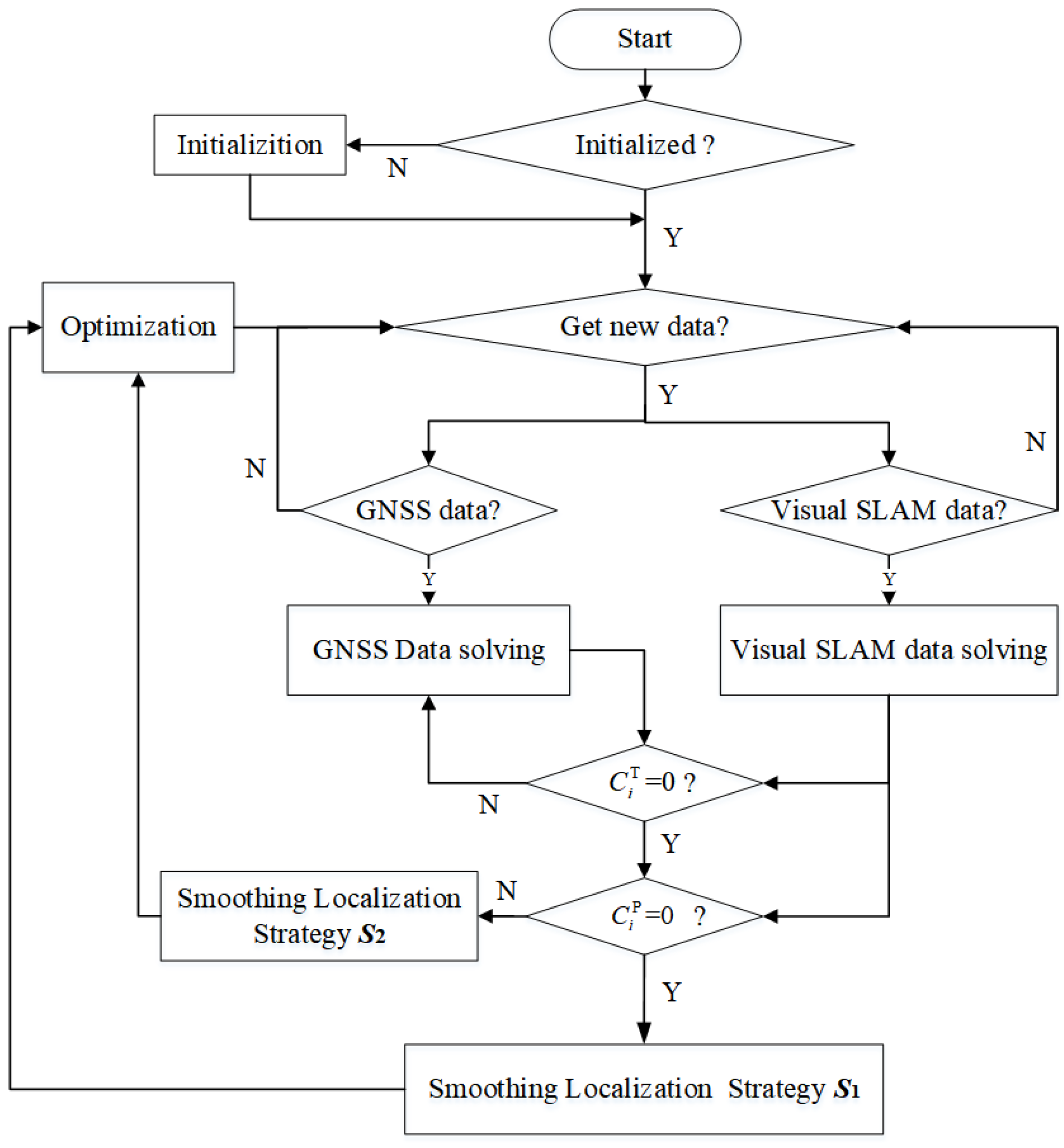
After the constrained optimization of Equation (33), the coordinates of the mobile terminal are finally obtained, which are the localization results of the GNSS/Visual SLAM system to the mobile terminal calculated by the smoothing localization method. A flow-chart of GNSS spoofing identification and smoothing localization method is shown in Figure 4.
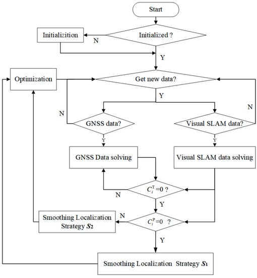
Figure 4.
Flow-chart.
4. Simulation results
4.1. Experimental Conditions and Data Set
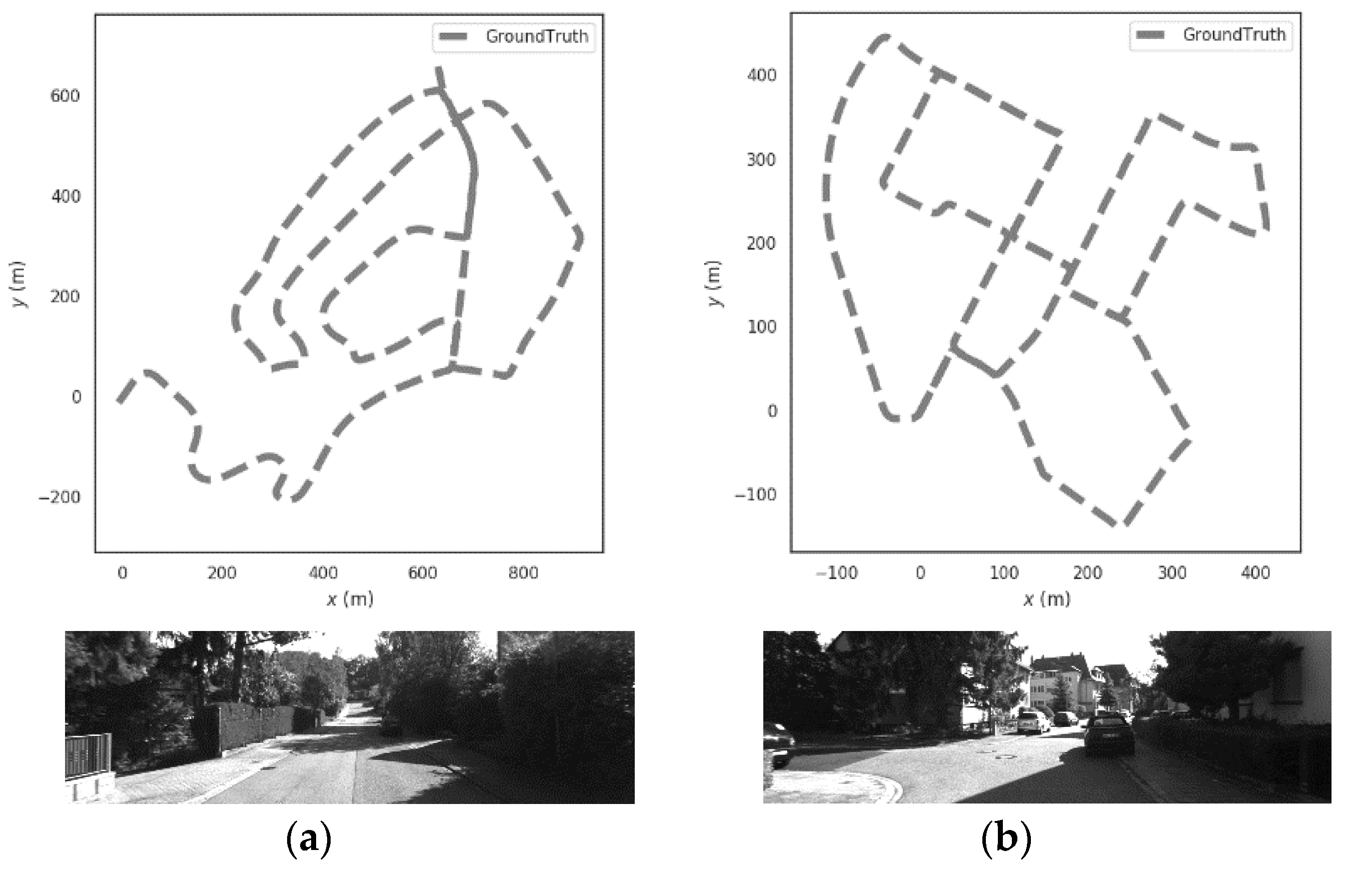
In order to analyze the proposed GNSS spoofing identification and smoothing localization method based on GNSS/Visual SLAM system (referred to as PTC-SLM), this paper selects the commonly used autonomous driving data set KITTI [24,25] for simulation verification and performance evaluation. The rural and urban scenes in the KITTI datasets are used, and the ground-truth of the two scenes are shown in Figure 5. The sensors we use are a GNSS navigation system and a binocular vision system composed of two identical gray-scale cameras. The parameters of sensors are shown in Table 1.

Figure 5.
Trajectories of ground-truth in (a) rural and (b) urban scenes.

Table 1.
List of sensor simulation parameters.
In order to verify the proposed PTC-SLM method, we performed a spoofing simulation on the GNSS data in the two KITTI datasets. From the analysis in Section 3.3, it can be seen that the performance of GNSS spoofing in the mobile terminal is the deviation of the localization domain. In the spoofing process, since the spoofing terminal does not know the destination of the terminal, in order to deceive the terminal to the target point, it is necessary to adjust the magnitude of the spoofing distance when each spoofing signal is sent. Therefore, the GNSS spoofing attack shown in Equation (34) is injected into the GNSS measurement data in the KITTI dataset.
where and are the actual measurement longitude and latitude of the terminal at time i, is the longitude error at time i and is the latitude error at time i. In our forwarding spoofing simulation, we pull the terminal to a place parallel to the actual direction of travel, then the spoofing distance becomes a fixed value (). In our inducing spoofing simulation, we gradually induce the terminal, so that every moment the spoofing terminal will increase the spoofing distance by a small displacement. Assume that the spoofing superimposed by the spoofing terminal is linearly increasing and assume the spoofing starts at time , then the cumulative drift of inducing spoofing at time is
where and are the distance of spoofing superimposed in the longitude and latitude directions. After the spoofing attack is injected, the localizations of the mobile terminal are gradually deviated from the correct track. If the GNSS spoofing is not detected in time, the mobile terminal is likely to be kidnapped on other paths or directly damaged by a collision accident. Next, we analyze the parameters of the PTC-SLM method to confirm that the time and localization verification parameters are reasonable.
4.2. Parameter Analysis
This section analyzes the impact of time verification threshold and localization verification threshold on our proposed PTC-SLM method. Whether it is a time verification threshold or a localization verification threshold, it is related to the frequency and accuracy of the sensors in practical applications and possible spoofing scenes.
Under our experimental settings and scenes, first of all, for the time verification threshold , the GNSS frame rate for the KITTI data set we selected is 10 fps, that is, the interval between two GNSS frames is 0.1s, then when , the window time is greater than 0.1s, there will be more GNSS frames that meet the time window requirements and enter the time verification process, which will cause data misalignment and increase the error of the method. Therefore, the time verification threshold must meet . So, we select to calculate the absolute position error (APE) of the PTC-SLM method, and the results are shown in Figure 6. Maximum value (Max), average value (Mean), median value (Median), minimum value (Min), rmse and std of the absolute position errors of the different time verification thresholds are shown in Table 2.
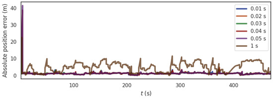
Figure 6.
The trend of APE under different time verification thresholds.
Table 2.
Error parameters of the different time verification thresholds.
It can be seen that the change of affects the results of APE. As increases, the rmse of the PTC-SLM method decreases first and then increases. When is too large (such as ), the result of APE is wobbly, and the time verification loses its effect; when , the result of APE is the smallest, so in subsequent experiments, the time verification threshold is selected as .
According to the analysis in Section 3.3, after the GNSS/visual SLAM system is combined, is related to the extreme error of the GNSS system and the extreme error of visual SLAM system which are related to the accuracy of the sensors in different systems. For the GNSS and visual SLAM system in the KITTI dataset, we first calculate the of the GNSS system and the of visual SLAM system separately through simulation when there is no GNSS spoofing occurs (). Then, substitute the value into Equation (19) and obtain the joint probability of the GNSS/visual SLAM system, as shown in Figure 7.
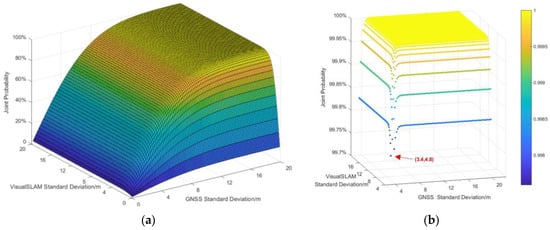
Figure 7.
The joint probability density distribution of the GNSS/visual SLAM system. (a) Total joint probability, (b) Joint probability greater than 99.37%.
From the simulation results of the joint probability density distribution, it is known that the confidence interval for the joint probability density of the GNSS/visual SLAM system to be greater than 99.37% is . That is, the limit error of the GNSS system is , the limit error of the visual SLAM system is . Therefore, according to Equation (30), the localization verification threshold of the system is calculated as .
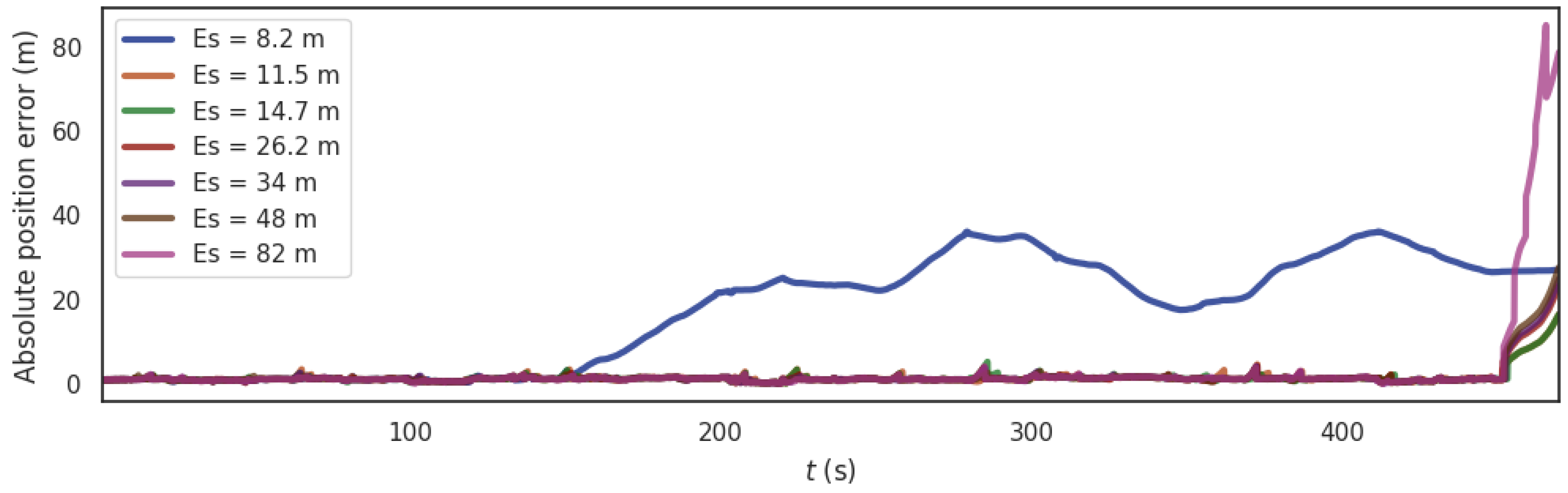
In order to analyze the influence of the location verification threshold of forwarding spoofing on the algorithm, the segment from 380 s to 410 s of the data set is exposed to a GNSS forwarding spoofing with 10m spoofing distance. Then, we select according to several extreme values of the system and performed simulations (, , , , , , ). At the same time, we applied a spoofing offset to GNSS system and analyzed the absolute position error (APE) of the PTC-SLM method with different localization verification thresholds. The APE simulation result is shown in Figure 8 and some error parameters of the different localization verification thresholds are shown in Table 3.

Figure 8.
The trend of APE under different localization verification thresholds of forwarding spoofing.
Table 3.
Error parameters of the different localization verification thresholds of forwarding spoofing.
It can be seen that the change of affects the trend of APE under different localization verification thresholds. With the increase of , the rmse of the APE changes from large to small and then increases. When the value of localization verification threshold is very small (for example ), the PTC-SLM method will diverge during the initialization phase, making the initialization of the GNSS/Visual SLAM system fail, causing the PTC-SLM method invalid. When and , after being spoofed by GNSS spoofing terminal, the Visual SLAM system has been spoofed by GNSS due to detection failure. When GNSS spoofing stops, the offset of GNSS data frame exceeded the threshold, false alarms continue to occur. When the value of localization verification threshold is very large (for example ), the PTC-SLM method cannot detect GNSS spoofing and the method is invalid. Therefore, the minimum distance of GNSS spoofing that our method can detect is limited to . Among them, when , the absolute error of the method is the smallest, which is consistent with the theoretical analysis. So we set the localization verification threshold as in the subsequent experiments.
In order to analyze the influence of the location verification threshold of inducing spoofing on the algorithm, the segment from 450 s to 460 s of the data set is exposed to a GNSS inducing spoofing (a 0.5 m distance is superimposed at each GNSS localization moment). We assume the size of the window W is 10. Then, we selected according to several values of the system and performed simulations (, , , , , , ). The results of absolute position error (APE) under the PTC-SLM method with different localization verification thresholds of inducing spoofing are shown in Figure 9 and some error parameters of the different localization verification thresholds are shown in Table 4.
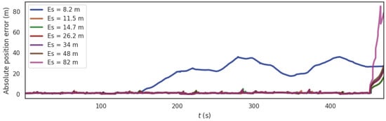
Figure 9.
The trend of APE under different localization verification thresholds of inducing spoofing.
Table 4.
Error parameters of the different localization verification thresholds of inducing spoofing.
It can be seen that the change of affects the trend of APE under different localization verification thresholds. With the increase of , the rmse of the APE changes from large to small and then increases. When is small (for example ), the cumulative error calculated by PTC-SLM exceeds the threshold due to the influence of sensor cumulative measurement errors. When there is no induced spoofing, false alarms occur and cause normal GNSS frames to be discarded and the localization results of visual SLAM system will produce cumulative errors because there is no GNSS frame to optimize the absolute position. When is large (for example, ), the PTC-SLM method cannot detect GNSS spoofing in time, and missed detection occurs, so that the localization result of PTC-SLM is induced by the GNSS spoofing and large errors are generated. Among them, when , PTC-SLM can detect GNSS induced spoofing in time, and its absolute error is the smallest, which is consistent with the theoretical analysis. Therefore, we set the localization verification threshold as in subsequent experiments.
5. Experimental Analysis under Forwarding Spoofing Attack
In order to verify the effect of the PTC-SLM method, we simulated two GNSS spoofing scenes of forwarding spoofing attack and induced spoofing attack. In this section, only the experimental analysis under the forwarding spoofing attack is analyzed. We try to compare PTC-SLM method with the GNSS method and VINS-Fusion method [7]. The GNSS method is the results of GNSS receiver and it will be directly affected after GNSS spoofing occurs. The VINS-Fusion method is a coupled algorithm of GNSS and visual SLAM. After GNSS spoofing occurs, the obtained spoofed GNSS results will enter the back-end optimization process, which will affect the final localization result of VINS-Fusion method. In the following passage, we compare the three algorithms in rural and urban scenes.
5.1. Rural
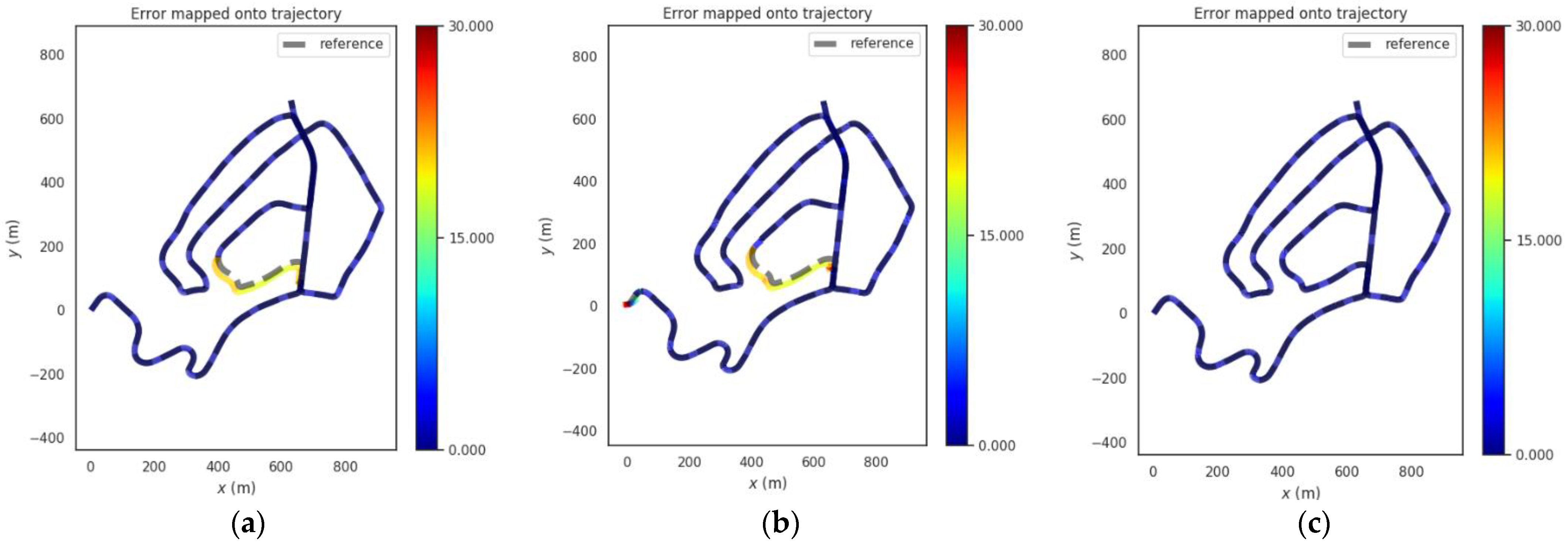
For the rural scene shown in Figure 5a, the segment from 100 s to 150 s of the data set is exposed to a GNSS spoofing with 20 m spoofing distance. Figure 10 shows the absolute position errors of GNSS, VINS-Fusion, and PTC-SLM after GNSS forwarding spoofing attacks. Figure 11 shows the trajectory of the three methods. Their maximum value (Max), average value (Mean), median value (Median), minimum value (Min), rmse and std of the absolute position errors of the three methods are shown in Table 5 below.
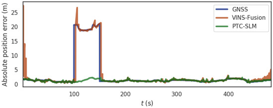
Figure 10.
The absolute position error of the three methods in rural scene.
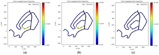
Figure 11.
Trajectories of the three methods in rural scene. (a) GNSS, (b) VINS-Fusion (c) PTC-SLM.
Table 5.
Error parameters of the three methods in rural scene.
It can be seen that when the GNSS method fails to detect GNSS spoofing attacks, the GNSS localization results are directly affected by GNSS spoofing, and the absolute position error of GNSS method grows immediately as the GNSS spoofing attacks occur as shown in the blue curve in Figure 10. The error on trajectory is shown in Figure 11a. The rmse of GNSS increased to 6.459 m.
The VINS-Fusion method uses GNSS and visual SLAM data to obtain the localization. With the injection of GNSS spoofing, the localization result of VINS-Fusion will gradually deviate from the normal track. When the GNSS attack is lifted, the localization result of VINS-Fusion will return to the normal track. The absolute position error is shown in the brown curve in Figure 10, and the error on the trajectory is shown in Figure 11b. The rmse of VINS-Fusion is 6.644 m.
The PTC-SLM method can detect GNSS forwarding spoofing attacks in time by inverting GNSS signals, and adopt a smoothing localization strategy to suppress the impact of GNSS spoofing. The absolute position error is shown in the green curve in Figure 10, and the error on the trajectory is shown in Figure 11c. It can be seen that the localization trajectory result basically coincides with the ground-truth (reference), and the rmse of PTC-SLM is 1.342 m, with an improvement of 79.223% compared with the GNSS method.
5.2. Urban
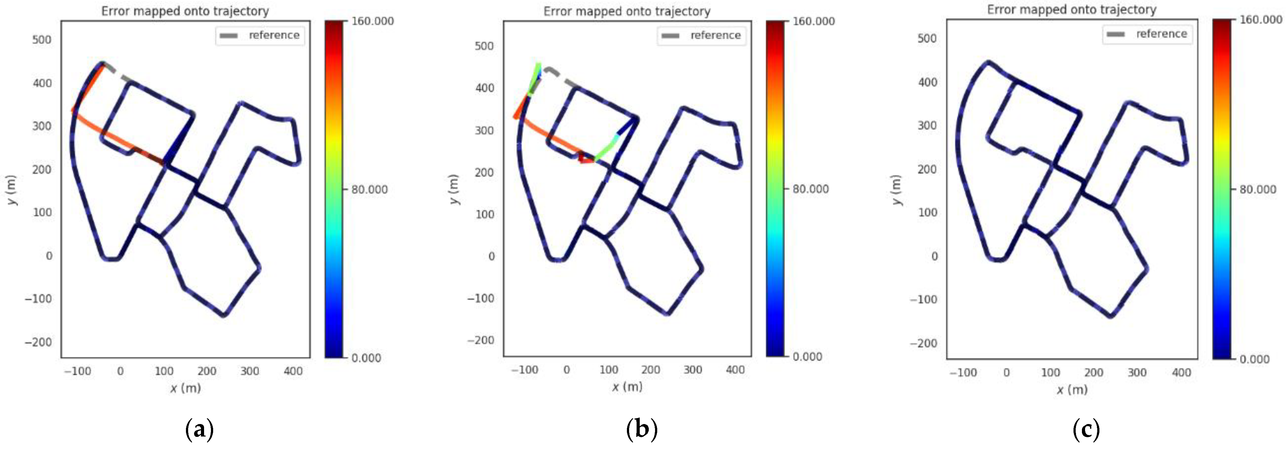
For the urban scene shown in Figure 5b, the simulation is the urban scene where the mobile terminal is spoofed and pulled to another road. So, we choose the segment from 380 s to 430 s of the data set and the terminal is exposed to a GNSS spoofing with 133 m spoofing distance, and the mobile terminal is simulated to be deflected to the adjacent road. Figure 12 shows the absolute position errors of GNSS, VINS-Fusion and PTC-SLM after GNSS forwarding spoofing attacks. Figure 13 shows the movement trajectory of the three methods of GNSS, VINS-Fusion, and PTC-SLM. Their maximum value (Max), average value (Mean), median value (Median), minimum value (Min), rmse and std of the absolute position errors of the three methods are shown in Table 6.
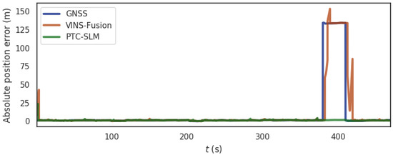
Figure 12.
The absolute position error of the three methods in urban scene.
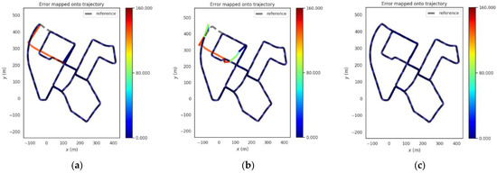
Figure 13.
Trajectories of the three methods in urban scene. (a), GNSS (b), VINS-Fusion, (c) PTC-SLM.
Table 6.
Error parameters of the three methods in urban scene.
It can be seen that when the GNSS method suffers GNSS forwarding spoofing, the GNSS localization results are directly affected by the GNSS forwarding spoofing and are incorrectly located on an adjacent road. The absolute position error of GNSS method is shown in the blue curve in Figure 12. The error on trajectory is shown in Figure 13a and the rmse of GNSS method increased to 33.918 m.
With the injection of GNSS forwarding spoofing, the localization results of the VINS-Fusion method will deviate from the normal track. When the GNSS attack is removed, the localization results after the VINS-Fusion method will oscillate and gradually return to the right track. The absolute position error is shown in the brown curve in Figure 12, and the error on the trajectory is shown in Figure 13b. The rmse of VINS-Fusion is 33.361 m.
The absolute position error of the PTC-SLM method is shown in the green curve in Figure 12. It can be seen that the PTC-SLM method is positioned smoothly, and the error on the trajectory is shown in Figure 13c. It can be seen that the localization result is still basically coincident with the reference, and the rmse is 1.579 m, with an improvement of 95.345% compared with the GNSS method.
6. Experimental Analysis under Inducing Spoofing Attack
In this section, only the experimental analysis under the GNSS inducing spoofing attack is analyzed in rural and urban scenes. We try to compare it with the GNSS method, VINS-Fusion method, and PTC-SLM-Forward method. The PTC-SLM-Forward method in this section is in the case where the PTC-SLM algorithm only considers forwarding spoofing identification (set to invalidate the induced identification) and can only identify forwarding spoofing but not induced spoofing. The PTC-SLM method in this section can identify both forwarding spoofing and induced spoofing.
6.1. Rural
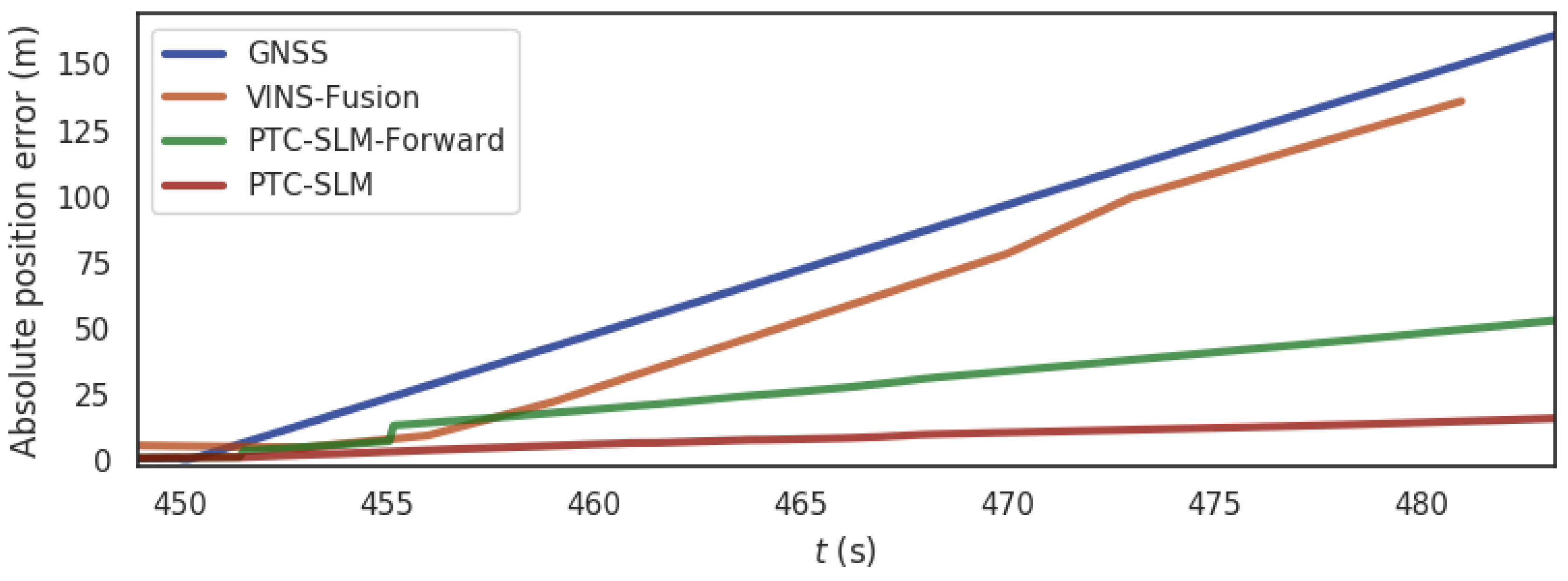
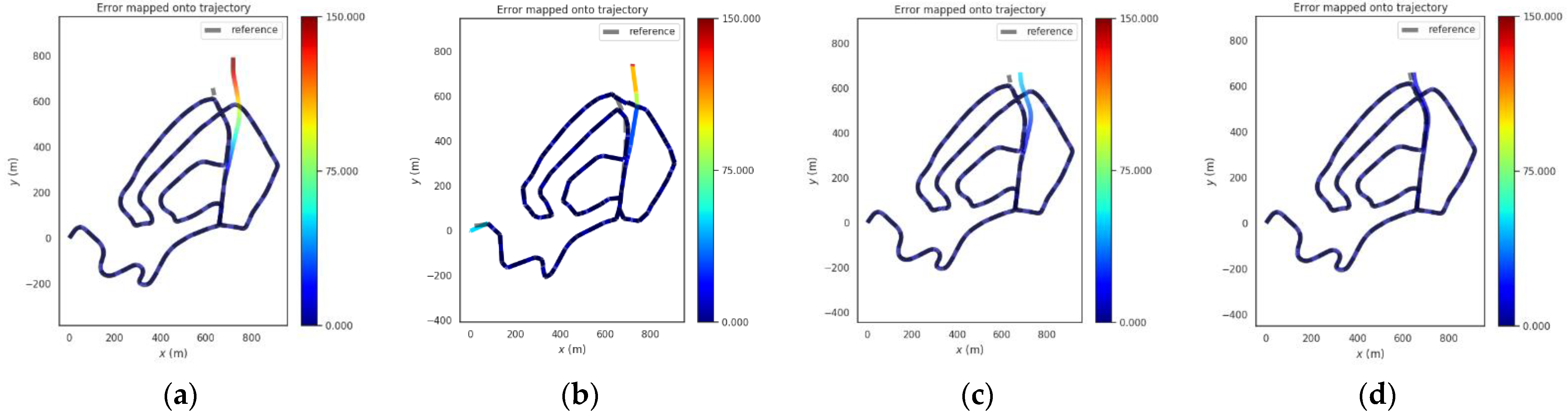
For the rural scene shown in Figure 5a, the segment from 450 s to 485 s of the data set is exposed to a GNSS inducing spoofing (a 0.5 m distance is superimposed at each GNSS localization moment). Figure 14 shows the absolute position errors of GNSS, VINS-Fusion, PTC-SLM (forwarding method only) and PTC-SLM after GNSS inducing spoofing attacks. Figure 15 shows the trajectory of the four methods. Their maximum value (Max), average value (Mean), median value (Median), minimum value (Min), rmse and std of the absolute position errors of the four methods are shown in Table 7.
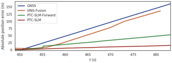
Figure 14.
The absolute position error of the four methods in rural scene.
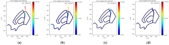
Figure 15.
Trajectories of the four methods in rural scene. (a) GNSS, (b) VINS-Fusion, (c) PTC-SLM-Forward, (d) PTC-SLM.
Table 7.
Error parameters of the four methods in rural scene.
It can be seen that the GNSS localization results are directly affected by GNSS inducing spoofing, and the absolute position error of GNSS method grows gradually as the GNSS inducing spoofing attacks occur as shown in the blue curve in Figure 14. The error on trajectory is shown in Figure 15a. The rmse of GNSS increased to 24.497 m. The localization result of VINS-Fusion will gradually deviate from the normal track and the absolute position error is shown in the brown curve in Figure 14, and the error on the trajectory is shown in Figure 15b. The rmse of VINS-Fusion is 21.191 m.
The PTC-SLM-Forward method did not identify GNSS inducing spoofing attacks in time but only when the forwarding spoofing deviation satisfy the constraints of . At this time, the method determines that forwarding spoofing has occurred. The absolute position error is shown in the green curve in Figure 14, and the error on the trajectory is shown in Figure 15c. It can be seen that the localization trajectory offset is smaller than the GNSS and VINS-Fusion methods, but larger than the PTC-SLM method. The rmse of PTC-SLM-Forward is 8.508 m, with an improvement of 65.269% compared with the GNSS method. The PTC-SLM method can detect GNSS inducing spoofing attacks in time to suppress the impact of GNSS inducing spoofing. The absolute position error is shown in the red curve in Figure 16, and the error on the trajectory is shown in Figure 17d. It can be seen that the localization trajectory offset is the smallest and the rmse of PTC-SLM is 2.870 m, with an improvement of 88.284% compared with the GNSS method.
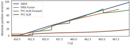
Figure 16.
The absolute position error of the four methods in urban scene.
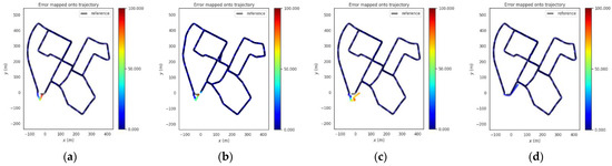
Figure 17.
Trajectories of the four methods in urban scene. (a) GNSS, (b) VINS-Fusion, (c) PTC-SLM-Forward, (d) PTC-SLM.
6.2. Urban
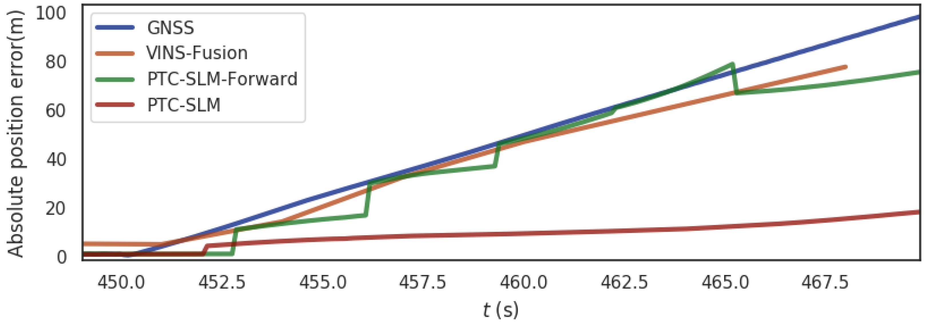
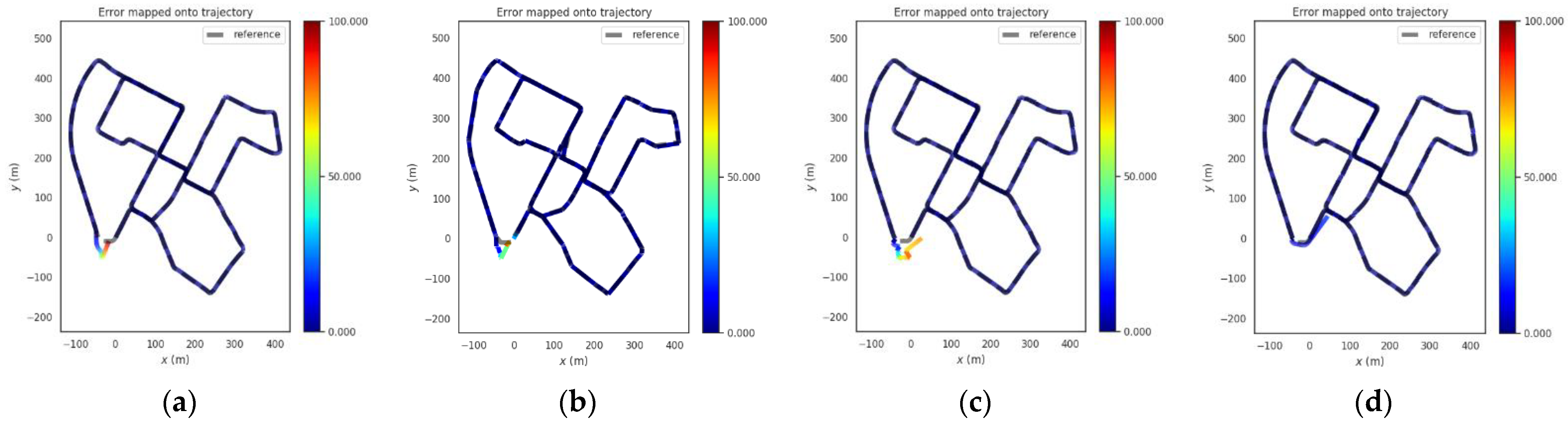
For the urban scene shown in Figure 5b, the segment from 450 s to 470 s of the data set is exposed to a GNSS inducing spoofing (a 0.5 m distance is superimposed at each GNSS localization moment). Figure 16 shows the absolute position errors of GNSS, VINS-Fusion, PTC-SLM-Forward, and PTC-SLM after GNSS inducing spoofing attacks. Figure 17 shows the movement trajectory of the four methods of GNSS, VINS-Fusion, PTC-SLM-Forward, and PTC-SLM. Their maximum value (Max), average value (Mean), median value (Median), minimum value (Min), rmse and std of the absolute position errors of the four methods are shown in Table 8.
Table 8.
Error parameters of the four methods in urban scene.
It can be seen that the absolute position error of GNSS method grows gradually as the GNSS inducing spoofing attacks occur as shown in the blue curve in Figure 16. The error on trajectory is shown in Figure 17a. The rmse of GNSS increased to 11.802 m. The localization results of VINS-Fusion gradually deviate from the normal track and the absolute position error is shown in the brown curve in Figure 16, and the error on the trajectory is shown in Figure 17b. The rmse of VINS-Fusion is 10.441 m.
The PTC-SLM-Forward method did not identify GNSS inducing spoofing attacks in time. The GNSS inducing spoofing is input into the smoothing localization process, so that the localization result obtained by the PTC-SLM-Forward method is continuously shift to the GNSS inducing localization direction. The absolute position error is shown in the green curve in Figure 16, and the error on the trajectory is shown in Figure 17c. The rmse of PTC-SLM-Forward is 10.399 m.
The PTC-SLM method can detect GNSS inducing spoofing attacks in time to suppress the impact of GNSS inducing spoofing. The absolute position error is shown in the red curve in Figure 16, and the error on the trajectory is shown in Figure 17d. When the GNSS spoofing is identified and the GNSS frame is discarded, the PTC-SLM method maintains the final localization output with the result calculated by the visual SLAM system and generates a visual cumulative error. It can be seen that the rmse of PTC-SLM is 2.477 m, with an improvement of 79.012% compared with the GNSS method.
Through the analysis results of Section 5 and Section 6, it can be seen that the PTC-SLM method can well identify GNSS forwarding spoofing and GNSS progressive spoofing and can obtain better smoothing localization results compared with other methods. Besides, the localization performance of PTC-SLM under forward spoofing attack is better than that under progressive spoofing attack.
7. Conclusions
This paper proposes a GNSS spoofing identification and smooth localization method for GNSS/Vision SLAM system. The time and localization results are offset of the GNSS data through the visual SLAM data, and it is identified whether the time and localization results of the GNSS exceed the time and localization verification threshold. According to the identified verification flags, different smoothing localization strategies are selected, and the localization results are optimized and adjusted using the sliding window to obtain smoothing localization results.
The selection of the time verification and localization verification threshold of the PTC-SLM method is related to the sensor performance (frequency and accuracy). For the selected sensors used in the KITTI datasets, we analyzed the selection of the time and localization verification threshold of the PTC-SLM method, and verified that the selection of the threshold is related to the sensor frequency and sensor accuracy.
In addition, two scenes in the KITTI datasets are selected for simulation and evaluation. In the simulation, we limited the size of the offset of the applied GNSS spoofing. By analyzing the performance comparison of the methods in different scenes, it is proved that the PTC-SLM method can identify the GNSS forwarding spoofing attacks and GNSS progressive spoofing attacks, and obtain smoothing localization results.
Author Contributions
Conceptualization, J.S., H.W. and T.L.; Data curation, X.G. (Xiaochen Guo), D.J. and H.L.; Formal analysis, J.S., X.G. (Xiaochen Guo) and D.J.; Investigation, X.G.(Xuqiang Guo) and T.L.; Methodology, J.S., H.W., D.J. and X.G.(Xuqiang Guo); Resources, T.L.; Software, X.G. (Xiaochen Guo) and H.L.; Supervision, H.W. and T.L.; Validation, X.G. (Xiaochen Guo) and X.G. (Xuqiang Guo); Visualization, H.W. and D.J.; Writing—original draft, J.S., D.J. and H.L.; Writing—review & editing, H.W., X.G. (Xiaochen Guo), X.G. (Xuqiang Guo) and T.L. All authors have read and agreed to the published version of the manuscript.
Funding
This research is funded by the Youth Innovation Promotion Association (E03315010D).
Institutional Review Board Statement
Not applicable.
Informed Consent Statement
Informed consent was obtained from all subjects involved in the study.
Data Availability Statement
Publicly available datasets were analyzed in this study. This data can be found here: [www.cvlibs.net/datasets/kitti] (accessed on 5 November 2021).
Acknowledgments
Not applicable.
Conflicts of Interest
The authors declare no conflict of interest.
References
- Servières, M.; Renaudin, V.; Dupuis, A.; Antigny, N. Visual and Visual-Inertial SLAM: State of the Art, Classification, and Experimental Benchmarking. J. Sens. 2021, 2021, 2054828. [Google Scholar] [CrossRef]
- Merzlyakov, A.; Macenski, S. Comparison of Modern General-Purpose Visual SLAM Approaches. In Proceedings of the 2021 IEEE/RSJ International Conference on Intelligent Robots and Systems (IROS), Prague, Czech Republic, 27 September–1 October 2021; 2021. [Google Scholar]
- Qin, T.; Li, P.; Shen, S. Vins-mono: A robust and versatile monocular visual-inertial state estimator. IEEE Trans. Robot. 2018, 34, 1004–1020. [Google Scholar] [CrossRef] [Green Version]
- Mur-Artal, R.; Montiel, J.M.M.; Tardos, J.D. ORB-SLAM: A versatile and accurate monocular SLAM system. IEEE Trans. Robot. 2015, 31, 1147–1163. [Google Scholar] [CrossRef] [Green Version]
- Mur-Artal, R.; Tardós, J.D. Orb-slam2: An open-source slam system for monocular, stereo, and rgb-d cameras. IEEE Trans. Robot. 2017, 33, 1255–1262. [Google Scholar] [CrossRef] [Green Version]
- Campos, C.; Elvira, R.; Rodríguez, J.J.; Montiel, J.M.; Tardós, J.D. ORB-SLAM3: An Accurate Open-Source Library for Visual, Visual–Inertial, and Multimap SLAM. IEEE Trans. Robot. 2021, 37, 1874–1890. [Google Scholar] [CrossRef]
- Qin, T.; Pan, J.; Cao, S.; Shen, S. A general optimization-based framework for local odometry estimation with multiple sensors. arXiv Prepr. 2019, arXiv:1901.03638. [Google Scholar]
- Cao, S.; Lu, X.; Shen, S. GVINS: Tightly Coupled GNSS-Visual-Inertial for Smooth and Consistent State Estimation. arXiv e-Prints 2021, arXiv:2103.07899. [Google Scholar] [CrossRef]
- Bhatti, J.; Humphreys, T.E. Hostile control of ships via false GPS signals: Demonstration and detection. NAVIGATION J. Inst. Navig. 2017, 64, 51–66. [Google Scholar] [CrossRef]
- Psiaki, M.L.; Humphreys, T.E. GNSS spoofing and detection. Proc. IEEE 2016, 104, 1258–1270. [Google Scholar] [CrossRef]
- Parkinson, S.; Ward, P.; Wilson, K.; Miller, J. Cyber threats facing autonomous and connected vehicles: Future challenges. IEEE Trans. Intell. Transp. Syst. 2017, 18, 2898–2915. [Google Scholar] [CrossRef]
- Junzhi, L.; Wanqing, L.; Qixiang, F.; Beidian, L. Research progress of GNSS spoofing and spoofing detection technology. In Proceedings of the 2019 IEEE 19th International Conference on Communication Technology (ICCT), Xi’an, China, 16–19 October 2019; pp. 1360–1369. [Google Scholar]
- Broumandan, A.; Lachapelle, G. Spoofing detection using GNSS/INS/odometer coupling for vehicular navigation. Sensors 2018, 18, 1305. [Google Scholar] [CrossRef] [PubMed] [Green Version]
- Yimin, W.; Hong, L.; Mingquan, L. Spoofing profile estimation-based GNSS spoofing identification method for tightly coupled MEMS INS/GNSS integrated navigation system. IET Radar Sonar Navig. 2019, 14, 216–225. [Google Scholar] [CrossRef]
- Song, J.; Wu, H.; Guo, X.; Li, S.; Gong, Y.; Zhang, Y.; Li, Y. Credible Navigation Algorithm for GNSS Attack Detection Using Auxiliary Sensor System. Appl. Sci. 2021, 11, 6321. [Google Scholar] [CrossRef]
- Xie, G. Principles of GPS and Receiver Design; Publishing House of Electronics Industry: Beijing, China, 2009; Volume 7, pp. 61–63. [Google Scholar]
- Lucas, B.D.; Kanade, T. An Iterative Image Registration Technique with an Application to Stereo Vision. In Proceedings of the 7th International Joint Conference on Artificial Intelligence (IJCAI’81), Vancouver, BC, Canada, 24–28 August 1981; Volume 8, pp. 24–28. [Google Scholar]
- Vidal, R.; Ma, Y.; Hsu, S.; Sastry, S. Optimal motion estimation from multiview normalized epipolar constraint. In Proceedings of the Eighth IEEE International Conference on Computer Vision, ICCV 2001, Vancouver, BC, Canada, 7–14 July 2001; Volume 1, pp. 34–41. [Google Scholar]
- Hartley, R.I. In defense of the eight-point algorithm. IEEE Trans. Pattern Anal. Mach. Intell. 1997, 19, 580–593. [Google Scholar] [CrossRef] [Green Version]
- Golub, G.H.; Reinsch, C. Singular value decomposition and least squares solutions. In Linear Algebra; Springer: Berlin/Heidelberg, Germany, 1971; pp. 134–151. [Google Scholar]
- Agarwal, S.; Mierle, K. Ceres Solver. Available online: http://ceres-solver.org (accessed on 15 May 2021).
- Wang, W.; Wang, J. GNSS induced spoofing simulation based on path planning. IET Radar Sonar Navig. 2022, 01, 103–112. [Google Scholar] [CrossRef]
- Umeyama, S. Least-squares estimation of transformation parameters between two point patterns. IEEE Trans. Pattern Anal. Mach. Intell. 1991, 13, 376–380. [Google Scholar] [CrossRef] [Green Version]
- Geiger, A.; Lenz, P.; Stiller, C.; Urtasun, R. Vision meets robotics: The kitti dataset. Int. J. Robot. Res. 2013, 32, 1231–1237. [Google Scholar] [CrossRef] [Green Version]
- Geiger, A.; Lenz, P.; Urtasun, R. Are we ready for autonomous driving? The kitti vision benchmark suite. In Proceedings of the 2012 IEEE Conference on Computer Vision and Pattern Recognition, Providence, RI, USA, 16–21 June 2012; pp. 3354–3361. [Google Scholar]


Publisher’s Note: MDPI stays neutral with regard to jurisdictional claims in published maps and institutional affiliations. |
© 2022 by the authors. Licensee MDPI, Basel, Switzerland. This article is an open access article distributed under the terms and conditions of the Creative Commons Attribution (CC BY) license (https://creativecommons.org/licenses/by/4.0/).