Abstract
The goal of any lean implementation in production process is achieving better production performances and one of them is productivity. Among many lean principles, pull principle is the most complex to achieve. There are different production control mechanisms for achieving pull and making decision which one to apply can be demanding because sometimes it is not obvious which is the best for specific situation. Many different production parameters influence production process and for one production setting, one control mechanism is the best choice, but for another production setting it might not be. One goal of this study was to research the influence of bottleneck in the production process in regard to achieving better productivity by applying pull principle. Some of the literature considered deals with the topic of bottleneck and pull but focuses only on bottleneck or in addition on one another production parameter and most of the literature studies up to three different pull control mechanisms. One of the objectives of this study was also to fill the research gap in a way to investigate more mechanisms, particularly, according to the literature, those most widely used in various production conditions with emphasis on bottleneck. The advantage of this research is that in addition to the bottleneck, other parameters, namely the number of control cards, variations and processing time are considered. For that reason, simulation experimentation was conducted and as a result regression functions modelling the relationship between productivity and mentioned parameters for four different pull control mechanisms are gained. The analysis showed that the existence of a bottleneck affects the effectiveness of pull mechanisms in terms of productivity.
1. Introduction
Digitalization and Industry 4.0. (I 4.0) are the latest trends in industry, specifically in managing and controlling production. However, evidently, well known methodologies for production management and improvement of production processes such as lean manufacturing, six sigma etc. are still important. Thus, authors [1] point that the only technological adoption which is characteristic of I 4.0 will not lead to distinguished results. Lean manufacturing practices help in the installation of organizational habits and mindsets that favor systemic process improvements, supporting the design and control of manufacturers’ operations management towards the fourth industrial revolution [1]. In addition, it is known that changes toward Industry 4.0 could be significant and any mistakes or skipped step could cause waste in the future [2]. It is obvious how lean manufacturing is still an important topic, both for research and practice.
Womack, J.P. and Jones, D.T. define five basic lean principles:
- Value;
- Value chain;
- Flow;
- Pull;
- Perfection [3].
Pull principle is the most complex principle for the company to achieve, mainly because many preconditions need to be satisfied in order to start with implementing this principle. Pull emerged from one of the most known paradigms of Toyota Production System (TPS) and that is Just-in-Time. (JIT). The idea behind Just-in-Time is to deliver the product to the customer as close as possible to when the customer requires it. Hopp and Spearman state that the Kanban is misunderstood as a synonym for pull and JIT production, when Kanban is rather just one of the means for achieving pull thus, is itself a pull control mechanism [4]. Later other pull control mechanisms have emerged.
The aim of this study was to research the influence of bottleneck on productivity with respect to different pull control mechanisms, in different production conditions defined by level of variations, number of pull control cards and processing time. The influence of lean manufacturing implementation on productivity is well described in literature [5,6,7,8,9]. Adoption of lean manufacturing results in an increase of productivity not just in production processes, but also in the design of a product. Hence, in [10], the case study of adopting lean in product design is presented and it is described that after adopting TPS principles the number of design cases undertaken by the design department increased [10].
However, how do pull control mechanisms affect productivity and how do they behave depending on whether that there is or there is not bottleneck in the process? Karrer [11] argue that production control mechanisms have a direct influence on delivery, and that is driven by production lead time and by the productivity.
On the other hand, bottleneck detection in manufacturing is the key to improving production efficiency and stability in order to improve capacity and thus productivity.
In Chu ans Shih’s work, [12], it is presented that some studies have found that simply increasing the number of Kanban cards (inventory level) cannot resolve bottleneck problems. Bonvik [13], researched three mechanisms Kanban, Conwip and Hybrid Kanban/Conwip in terms of bottleneck, but only how it affects the production lead time.
According to the relevant literature, the most widely used three control mechanisms are Kanban, Conwip and Hybrid Kanban/Conwip [14]. On the other hand, DBR mechanism was specially designed for processes with bottleneck [15]. There is a gap in research that might take into consideration multiple mechanisms in the context of the impact of bottlenecks on productivity. Therefore, the intention of this study was to answer the following research questions:
- Q1: Does the bottleneck affect the efficiency of the pull control mechanism (PCM)?
- Q2: Is the impact of the existence of a bottleneck on the efficacy of PCM different depending on the level of variability, processing time, as well as the level of work-in-process (defined by the number of PCM control cards in the process)?
1.1. Literature Review
1.1.1. Lean Manufacturing
Lean manufacturing is one of the major methodologies for production improvement and managing highly effective production processes. It has evolved from TPS. The interest for TPS in the western countries emerged after the success of the joint venture NUMMI of Toyota and General Motors, after which the book called The Future of Automobile was released. In a later book, The Machine that Changed the World, with the same focus of research, the book John Krafik uses the term lean for describing TPS for the first time [16,17]. Today Lean manufacturing is considered as production paradigm the goals of which are to produce value for the customer and to shorten the lead time of the production process [18,19]. The West adapted Japanese tools and principles to reduce waste, lead time and value for the customer. Thus, lean manufacturing in its early stage consisted of tools mainly for the shop floor. Later the paradigm of lean manufacturing or lean production evolved into the paradigm of lean thinking. This is why authors in [19] have made the distinction of lean thinking at the strategic level and lean thinking on the shop floor level, and they found that it is very important to understand lean on both levels, as a whole, in order to apply the right tools to provide value for the customer. They state that understanding lean thinking as only shop- floor methodology leads to a limited understanding of what contemporary lean approaches are about. According to those authors lean thinking has evolved from a production toolkit, through single supplier-customer focus dyad, to a strategic value proposition [19]. Thus, lean manufacturing both as a production toolkit, as well as strategic philosophy can be implemented in other environments, not just in manufacturing.
1.1.2. Lean Application in Different Industries
Over the years lean has evolved both as a toolkit and strategy for application in many different industries and types of organization. For example, possibilities of implementing lean in public sector, as well as its specificity are described in [20]. That research presented a case study of lean implementation in the Brazilian regulatory agency and revealed two decisive aspects in public environment; human and legal. Many times, these kinds of initiatives are dealing with legal aspects which involves slow bureaucratic processes; thus, these initiatives have to be supported by awareness and support of more decision makers other than managers willing to improve processes [20]. An interesting case study was presented by Jing, S. et al. The authors developed procurement value stream mapping as a tool of improving procurement process in manufacturing warehouse [21]. They showed improvement by this method in reducing business inventories, shortening the plan-making cycle, billing cycle, information cycle, logistics cycle a procurement cycle. Another application of values stream mapping, but in retail sector was presented in case study by Yanfang Qin and Hongrui Liu [22]. The authors presented that the methodology could improve supply chain management efficiency and customer satisfaction. Of lean implementations in public sectors the implementation in healthcare is the best explored. Implementation of lean in healthcare is well described in paper [23]. Authors described the successful implementation of lean tools in a French public hospital which has improved the quality of health services delivered to the patient. Another case study of lean implementation in healthcare is presented in paper by Antosz et al. [24]. They showed successful application of Value stream mapping (VSM), one of the widely used lean tools. Another application of VSM in healthcare system is presented in work of Cardoso [25]. The case study is undertaken in emergency care. The goal was to show the utilization of VSM for detecting wastes and improvement points. The result of proposed improvements implementation was shorter lead time. An interesting research regarding lean implementation in healthcare, but in outpatient departments was carried out by Ting Yu, Kudret Demirli and Nadia Bhuiyan, [26]. They have developed the framework to guide Lean transformation and solve the issues in outpatient’s department through identifying demand, coordinating resources, levelling schedules, and controlling wait times. Research [27] presented a literature review of implementation of lean in healthcare. The authors have reported the increase of papers dealing with lean in healthcare, however they found that the lack of continuous improvement throughout the whole organization exists, while most of the articles describe isolated implementation in different areas of organization. Thus, they suggested, there are more possibilities in spreading isolated initiatives on the whole organization and promotion of cultural changes in context of lean. As lean evolved as a philosophy, its application became wider. One example of the successful application of lean is in the pharmaceutical industry, especially in the laboratory as presented in the article [28], which showed the success of the use of lean in this area. The authors have found three types of waste; transport, waiting and defects to comprise almost 51.4% of the problem regarding lean assessment of the laboratory. Interesting case study, also in pharmaceutical industry was presented by Byrne et al [29]. The goal of the study was to reduce downtimes by applying Lean Six Sigma tools. The results of application of lean and six sigma tools were elimination of downtime, improvement of production flow, higher productivity as well as reduced backlog and elimination of product wastage.
Lean research in automotive industry is still valuable and up to date. Recent study carried out by Gaspar and Leal study [30], describes application of shop floor management model as presented by Hanenkamp, and defined a guideline dealing with sustainability of lean tools and philosophies in a manufacturing environment. Another study presented by Jagmeet Singh and Harwinder Singh [31], describes implementation of value stream mapping in a manufacturing company which is producing automotive suspension and fastening components and proved process improvement in terms of cycle time and level of work in process. Application of lean tools for waste reduction in steel industry is described in case study by Furman and Malysa [32]. A case study of lean implementation in plastic industry, specifically application of SMED (single minute exchange of die), lean tool for reduction of preparation time is presented by Reyes et al. [33]. The authors of a study conducted in Mexico also argue that lean is still one of the most important approaches in improving production [34]. They developed an instrument based on critical success factors to evaluate the implementation of lean tools, specifically in this study, for transportation equipment manufacturing subsector. Research about importance of implementation of lean and critical factors for implementing lean in Iranian industry was presented by Zahrae [35].
Lean has proven successful also in construction and shipbuilding industry. The authors of [36] have described the case study of implementation of lean in the bidding phase of construction process and found that it can benefit from lean. Lean has also found its application in the shipbuilding industry. Avad et al. have presented the study of possibilities of lean thinking implementation in construction industry. The objective was to improve building productivity. Results of productivity improvements with the approach presented were more sustainable as well as the cost and waste reduction [37]. The case study of introducing lean practice in the Croatian shipbuilding industry, by value stream mapping is presented in [38]. What the barriers of implantation of lean in shipbuilding industry are, specifically on the example on the shipbuilding industry in Singapore is well described in research paper [39]. Authors tried to explain the barriers to lean manufacturing as well as provide guidance for adopting lean practice in the shipbuilding industry.
In order to help various industries in implementing lean, a very interesting question is which lean tools and methods help the most to achieve the organizational goal. Thus, [40] have conducted review of 70 articles in 21 journals and have found that value stream mapping and DMAIC are the most widely used tools in all types of industries. They are followed by SMED and 5S. DMAIC is basically Six Sigma tool, while all other mentioned are lean tools. These findings could help other companies in deciding which direction to take when considering implementing lean [40].
1.1.3. Lean and Productivity
The goal of any lean implementation is to improve the organization processes and the efficiency of processes, which can be measured by productivity. The implementation of lean in small and medium enterprises and how it affected production productivity is presented in [5]. Authors have reported productivity improvement of productivity by 3900 additional units per month. In [6] authors presented a case study of applying lean in medium scale pump manufacturing. After adopting various lean techniques, mainly, value stream mapping, takt time and line balancing, authors reported improvement of assembly line efficiency up to 97%, as well as reductio of lead time about 13%. A similar case study of the application of lean production in small series production company is presented in [7]. After analyzing and eliminating waste, productivity has been improved, as well as lead time [7]. The application of lean tools, value stream mapping and waste elimination in the context of increased productivity is presented also in [8,9].
1.1.4. Pull Control Mechanisms
As previously explained, in practice, Kanban is often the first association when pull principle is considered. It was developed from the beginning of TPS [3], and later, when TPS started to spread in western countries and different types of manufacturing industries, other pull mechanisms were developed. Three of them, besides the Kanban, are the focus of this study and they are Conwip, Hybrid Kanban/Conwip and DBR.
Conwip was developed by Spearman et al. [41]. It is a pull mechanism that limits the total amount of work in process as communication cards only exists between the finish goods warehouse and the first operation, whereas in Kanban communication cards flow between every workstation (every operation) upstream in the production process. Conwip is the abbreviation of “Constant Work in Process”, the name that describes the essence of this pull mechanism [41].
Bonvik et al. proposed a new mechanism and called it Hybrid Conwip/Kanban as it combines communication rules both from Conwip and Kanban, thus communication exist both between warehouse and the first station but also between every station upstream in the process. They state that the advantage of the Hybrid Conwip/Kanban is in the processes with more workstations and more variability in the process but also the processes with bottleneck [13].
DBR is developed by Goldratt in his Theory of Constraints. The idea is that the signal for the beginning of processing a new item is sent from the bottleneck buffer to the first workstation in the production process [15].
While some of the studies of pull mechanisms investigate single-stage production processes [42] others investigated multistage processes, mostly with single product production [43,44,45,46,47]. Some articles describe case studies of implantation of pull control mechanisms [48] describes the development of two different Conwip approaches for bicycle chain manufacturing. They have simulated and compared these two approaches with the existing one and found that one outperforms by 42 percent and another by 50 percent regarding lead time. In [49] a case study of implementation of Hybrid Kanban/Conwip mechanism in high-variety/low-volume production process is presented and an increase of 38 percent in inventory turnover is described.
In addition, majority of studies deal with discrete production systems, but interesting findings regarding pull and its possibilities for process industry are presented in the research of Stevenson and Found who have gained important insights into the importance of pull and flow in process industries and its impact on production service, waste and utilization [50]. Very useful findings were gained in the study by Gayer et al. who researched applicability of pull in three different contexts, namely manufacturing, healthcare and construction. They have developed a method for assessment of pull production system according to twenty-three parameters divided in three groups: design, stability, and control [51]. In addition, Aldas et al. have investigated Kanban, Conwip and DBR by simulating production process in the textile industry and concluded with the preference of Kanban over Conwip and DBR [52]. Piplani and Ang, [53], compared Base Stock, Traditional Kanban Control System and Extended Kanban Control System (both dedicated and shared type) by simulation using common total cost measure as a performance measure for comparison. They presented procedures for optimizing multiple product Kanban control systems Numerical results show that the dedicated and shared-extended Kanban control systems outperform the other two systems [53].
2. Materials and Methods
Since the focus of this study was to investigate the influence of bottleneck on productivity of production processes controlled by different pull mechanisms, first the pull mechanisms themselves had to be defined. Bicheno found that Kanban, Conwip and DBR are three the most widely used pull production control mechanisms [14]. Review of the literature revealed the advantages also of Hybrid Kanban/Conwip; thus, these four mechanisms were researched in this study.
Kanban in Japanese means “card”, and in TPS it was used to manage flow of material through the production process. In the production process controlled by Kanban cards, production is triggered by a demand. The operation stations send the signal (Kanban card) to the upstream workstation to replace the part that was just used. Hopp and Spearman argue that there is a difference in installing and implementing Kanban and that the Kanban is very often considered as simple, but they state that the idea of Kanban is simple, and implementation is not. That is so because there are prerequisites for implementing Kanban in the process [54].
If production line consisting of two workplaces (two stages of the production process) where the process is controlled by a simple Kanban control mechanism is considered, the process of production control look as follows.
In the initial state, in the i-th stage of the production process, the Bi buffer contains ki semi-finished products, where each semi-finished product has one Kanban card attached. When the demand from the customer arrives, the request goes to line D and withdraws the finished product from B2. At this point, there are two possibilities:
- If there is a finished product in B2, it is forwarded to the customer after the Kanban k2 previously attached to it is separated from it. That Kanban is transferred to buffer of Kanban cards, K2, which is a signal to produce a new piece of semi-finished product in stage 2;
- If there is no finished product in B2, the request is withdrawn and put on hold until the finished product arrives in B2. As soon as the finished product arrives, it is delivered to the customer and Kanban goes to K2;
When the Kanban card arrives in K2 it authorizes the start of production of a new product in stage 2. Here, again, two situations can occur:
- If a semi-finished product is available in the B1 buffer, Kanban k1 is immediately removed and k2 is attached to that product. Then, the product and k2 go together to workplace 2. Kanban k1 is transferred to K1 buffer which authorizes starting production on WP1;
- If a semi-finished product is not available in the MS1 buffer, Kanban card of the stage 2, k2, will wait until new semi-finished product is available in MS1 [55];
As in the Kanban system, in Conwip system signal cards control the level of WIP. Only, the signal cards do not go from one workstation to another, that is from one buffer to another, but from the last buffer (warehouse) to the first workstation Thus, Conwip cards control the overall amount of WIP, in contrast with Kanban mechanism controls WIP on every workstation.
Figure 1 represents the DBR mechanism, which is similar to Conwip, only the control cards do not travel from the last buffer to the first workstation, but from the bottleneck buffer to the first workstation, thus if the bottleneck is on the last workstation, then the DBR has similar characteristics (similar route) as Conwip.
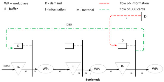
Figure 1.
DBR control mechanism.
Hybrid is a combination of Kanban and Conwip, thus signal cards follow the same route as in Conwip, which is the global flow of information and also there is a route of the cards as in the Kanban system which is the local flow of information.
In order to answer the research questions simulation experimentation was conducted. Simulation is a commonly used research methodology. It is useful when the analysis on a real system is not possible due to one of the many possible reasons, such as time constraints, complexity, or unavailability of the real system at the given moment. Simulation allows for repeated observations of a model, by setting up the experiment, knowing where input conditions can change, and then initiating a set of simulation executions that produce a set of results [56]. In this research Design of Experiments and Response surface methodology was used. It is statistical method for setting and analyzing experiments, with the goal of analyzing the response, thus the dependent variable, by varying the factors or the input variables that are independent and controlled by experimenter [57]. After running experiments, mathematical models of regression functions are generated in order to show the relationship between productivity of production process, i.e., that is dependent variable in this case, and independent variables which are going to be described further in the text.
2.1. Simulation Model
The decision on the simulation model was made based on literature review, and it was found that the five-workstations production line can present enough different problems and relations in production processes [58,59,60]. One such model was used in a paper by Enss and Rogers and was used for validation [61]. The assumptions for the model are described below.
Every workstation is a different production operation. Between each operation, there is a buffer in which semi-finished products are stored after processing in the corresponding operation. Processing route of parts are as follows: production process starts at workstation 1, then it continuous, respectively, on workstations 2, 3, 4 and 5. The production sequence follows the FIFO (first in-first out) rule. Production is organized as a one-piece flow. The process never starves for material and finished products can immediately leave the process. Transport time between workstations is negligible, so it is for transfer of Kanban, Conwip and DBR cards. The Kanban system is modeled as a single-card Kanban system. The processing time on every workstation was 60 min, as in the paper [61]. This processing time can be found in studies dealing with similar problems [46,47,61,62,63] A lognormal distribution was used to generate processing time values. Possible stoppages are modeled by the randomness of production time. The set-up time is not the subject of this research, since the single product production is observed. Simulation run was 117,000 h (corresponds to one year). These assumptions are consistent with the previous studies [58,61,64,65,66]. Simulation was conducted in software Matlab, in its features for simulation Simulink and Simevents [67]. Simevents is a feature in Simulink for discrete simulation.
Validation of the Model
For the validation of the simulation model, three validation techniques ware performed. The first one is Comparison to other models technique and the other one is Extreme condition test technique. Furthermore, all models were confirmed by Face validation in the way that colleagues from the same field of research examined them and confirmed their validity [64].
Since in the Enss and Rogers paper Push and Conwip were modeled, in the model for this study, first the Conwip was modeled with the same set up and that is that processing time was stochastic and defined by coefficient of variation cp. The distribution used was Gamma distribution. The number of Conwip cards was set to be the same [61]. The results of comparison are shown in the Table 1.

Table 1.
Validation of the model.
Kanban, Hybrid Conwip/Kanban and DBR were validated by Extreme condition test. The first extreme condition was extremely long operation time on the second workstation (85,000 min which is 80% of the whole simulation run). The results for every mechanism were that only one product came out of the process which is expected since the second operation took 80% of time of the simulation run. The second extreme condition was setting the number of control cards to zero at the one workstation in the case of Kanban and Hybrid, and in the case of DBR, extreme condition was the overall number of cards set to be zero. In every case the output was zero, meaning that no product was produced and that was expected since there were no cards that would trigger the production. All of these results feed into the assumption that the production process was well modeled.
2.2. Experiment Set Up
Since the focus of this study was the influence of bottleneck on productivity of production process controlled by different production control policies, bottleneck was the main independent variable. The other independent variables ware variability of production process, processing time and number of control cards of a pull control mechanism. Variability was expressed by the coefficient of variation.
One of the reasons the variability and the number of cards is chosen as a factor of the influence is strong relation between the variability (variable cycle time) on productivity [11]. Particularly, if the production process has variable cycle time influenced by many reasons, buffers (which are defined by the number of control cards in the process) provide production flow without stoppages in a way that it prevents the customer operation starving with material to process if the supplier operation is in shortage. In addition, it prevents stopping supplier operation if the subsequent operation cannot process a new part [11]. This is why variability is one of explored factors in this simulation study, as well as that number of control cards that define the level of WIP.
The levels of input parameters are shown in Table 2. The range of parameter value levels are consistent with those presented in literature [65,66].
Table 2.
Factor levels.
In order to define the relationship between parameters and response function simulation experiments are obtained and design of experiments is used. The Response surface method is applied to obtain mathematical model that define these relationships. According to Myers, Montgomery and Andersoon-Cook, [68], there is no standard response surface design for the case when some of the variables are categorical variables. In this case general full two-level factorial design was conducted and in Design-Expert 7, software used for making design and perform analysis, the design for combination of categorical and numerical variables is multilevel categorical [69]. Since there are four input parameters for this experiment, and five replication of two-level factorial design, 80 runs for each pull control mechanism were performed. This number of runs was performed for all four mechanisms, thus in total 320 runs was carried out. The order of execution of the experiment plan was random and generated by the Design-Expert 7 program. In Appendix A and Appendix B are presented experimental tables (Table A1, Table A2, Table A3, Table A4, Table A5, Table A6 and Table A7) which present all runs with standard order generated by Design expert, as well as responses gathered trough simulations. Due to the characteristics of the simulation model, the number of cards in the experiment are defined per workstation. Thus, for a total of 10 cards in the process, since the process consists of five workstations, the value of this parameter is two cards per workstation. For the case of 15 cards in the process, the value of the parameter is three cards per workstation (Appendix A).
3. Results
In this chapter the results of data analysis will be presented. The results speak of the dependence of productivity on bottleneck, variability, processing time and the pull control mechanism, specifically, the number of control cards for each mechanism. The data gathered by simulation experimentation were processed in order to obtain a mathematical model that describes that dependence. A total of eight regression functions were generated, two for each of the mechanisms (one for the process with bottleneck and one for the process without bottleneck), respectively, for Kanban, Conwip, Hybrid and DBR.
Analysis of variance (ANOVA) was performed to determine the significance of the factors and the response function was developed by regression analysis. The factors of model A, B, C and D were as follows:
- A—coefficient of variation.
- B—operation time;
- C—existence of a bottleneck;
- D—number of control cards.
For every mechanism, a table of analysis of variance (ANOVA) shows that the models are significant (Table 3, Table 4, Table 5 and Table 6). This is indicated by F-value, but also p-value. So, the hypothesis that variability, processing time, bottleneck and number of control cards do not affect the productivity is rejected. p-values for every parameter of the model showed significance of the parameters but also some of their interactions (Table 3, Table 4, Table 5 and Table 6).
Table 3.
ANOVA-Kanban.
Table 4.
ANOVA-Conwip.
Table 5.
ANOVA-Hybrid Kanban/Conwip.
Table 6.
ANOVA-DBR.
The deviations of the models, as seen in the tables were not significant, which was indicated by F-value, meaning that the models describe the phenomenon well enough.
After the analysis of variance, regression analysis was carried out for all mechanisms. All the values gather by regression analysis indicated significance of generated model and that the regression model is different from a random phenomenon. [69].
The generated model for Kanban was as follows:
PKanban-BN = 9.85712 − 0.844392Cv − 0.150878T + 0.003959Nr + 0.008078CvT + 0.001504CvNr
PKanban = 13.13354 − 0.936188Cv − 0.200347T − 0.002739Nr + 0.003491CvT + 0.034448CvNr
Variable from Equations (1) and (2) are as follows:
- PKanban-BN—productivity for the process with bottleneck, controlled by Kanban, min;
- PKanban—lead time for the process with without bottleneck, controlled by Kanban, min;
- Cv—coefficient of variation;
- T—processing time;
- Nr—number of control cards;
Ratio of maximum and minimum measured values, in cases of Conwip and Hybrid Kanban/Conwip mechanism measured value was greater than 10, so transformation of data was required [69]. In this way, the homogeneity of variance over the experimental space is satisfied [70]. Data were transformed according to Equation (3).
y’ = (y + k)λ, k = 0, λ = 0.88 for Conwip, λ = 0.88 for Hybrid Kanban/Conwip
Variables in the Equation (3) are:
- y’—transformed value
- y—real value
Regression functions for Conwip and Hybrid Kanban/Conwip mechanism are:
(PConwip)0.88 = 9.82046 − 0.877525Cv − 0.144614T − 0.036874Nr + 0.0051CvT + 0.117177CvNr + 0.000376TBr
(PConwip-BN)0.88 = 7.6239 − 0.584773Cv − 0.113088T − 0.025503Nr + 0.003642CvT + 0.029719CvNr + 0.000376TNr
(PHybrid)0.81 = 8.16982 − 0.563684Cv − 0.116823T − 0.008266Nr − 0.004897CvT + 0.066395CvNr − 0.000215TNr + 0.001038CvTNr
(PHybrid-BN)0.81 = 6.43031 − 0.231142Cv − 0.092833T + 0.008571Nr − 0.002235CvT − 0.036615CvNr − 0.000215TNr + 0.001038CvTNr
Variable from Equations (4)–(7) are as follows:
- PConwip-BN—productivity for the process with bottleneck, controlled by Conwip, min;
- PConwip—productivity for the process with without bottleneck, controlled by Conwip, min;
- PHybrid-BN—productivity for the process bottle neck, controlled by Hybrid Kanban/Conwip, min;
- PHybrid—productivity for the process with without bottle neck, controlled by Hybrid Kanban/Conwip, mi n;
- CV—coefficient of variation;
- T—processing time;
- Nr—number of control cards;
The values calculated by Equations (4)–(7) must be transformed by the Equation (8).
Regression functions for DBR mechanism are
PDBR-BN = 9.88346 − 0.696599Cv − 0.151325T − 0.004601Nr + 0.005583CvT + 0.016574CvNr
PDBR = 13.16724 − 0.961586Cv − 0.201172T + 0.004601Nr + 0.005583CvT + 0.016574CvNr
Variable from Equations (8) and (9) are as follows:
- PDBR-BN—productivity for the process with bottle neck, controlled by DBR, min;
- PDBR—productivity for the process with without bottle neck, controlled by DBR, min;
- CV—coefficient of variation;
- T—processing time;
- Nr—number of control cards;
4. Discussion
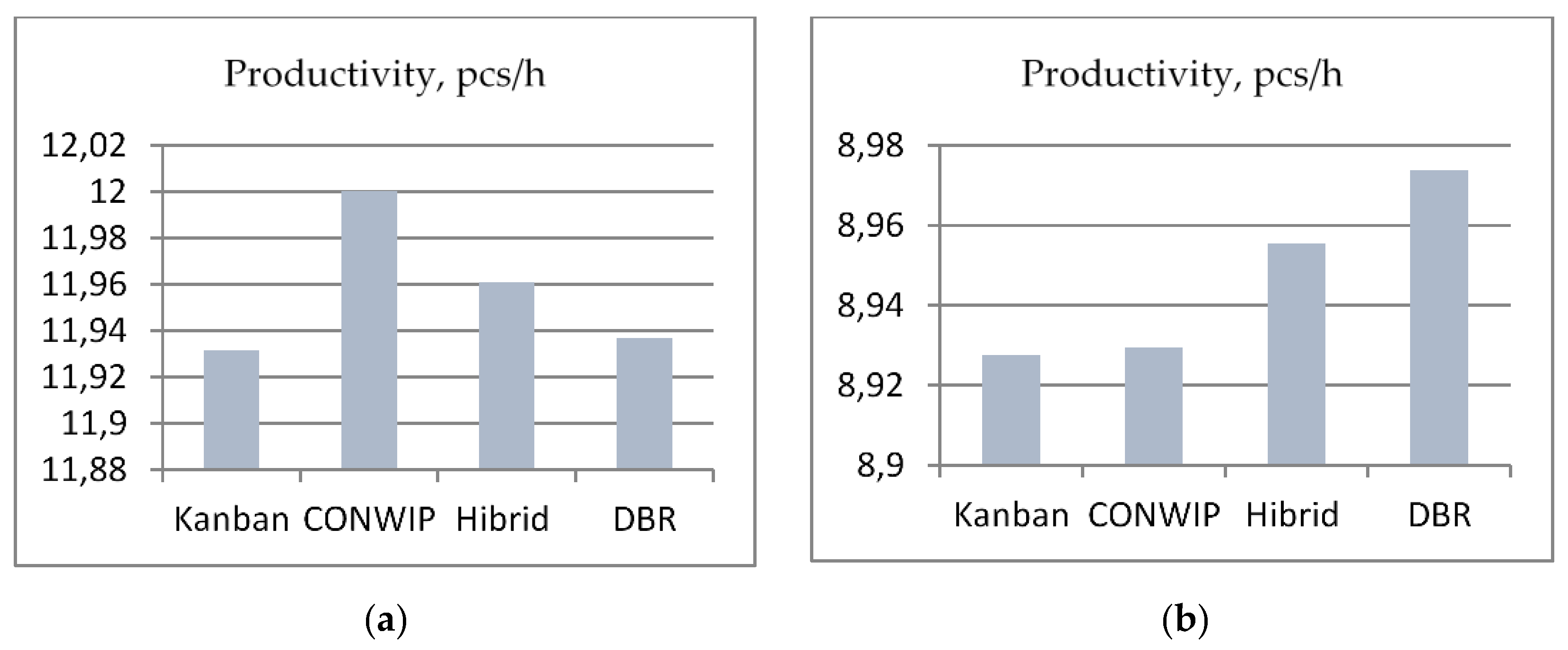
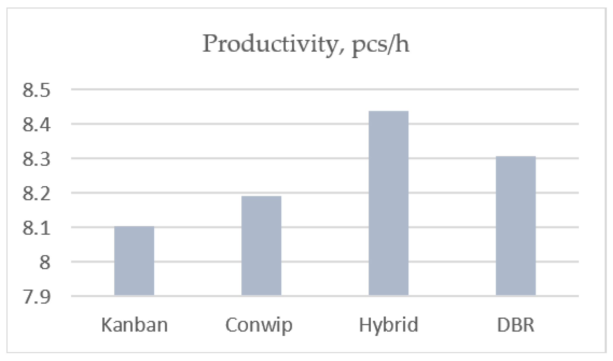
By using the regression function presented above, it is possible to calculate productivity levels for all four mechanisms, whether bottleneck exists in the process or not, and for a given current condition of a production process in terms of variability, processing time and the desired level of WIP. By comparing of calculated values, one can decide which control mechanism to choose. Figure 2 presents just one of the possible combinations of independent parameters and level of productivity for that specific condition. The influence of the bottleneck in the process is obvious and for the same level of parameters, variability, processing time and WIP, the same pull control mechanism will not achieve the optimal level of productivity in the process with and without bottleneck (Figure 2a,b). Therefore, for this specific case, for the process with bottleneck DBR would be better choice, while for the process without bottleneck the better choice would be the Conwip mechanism.
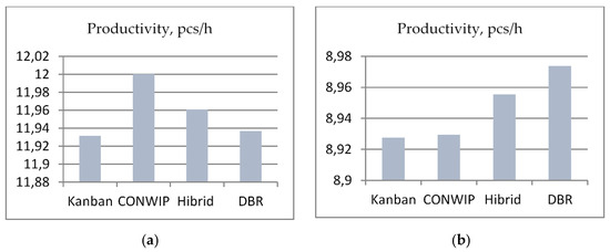
Figure 2.
Comparison of effectiveness of pull control mechanisms (a) Productivity for set of parameters: za Cv = 0.25, T = 5 min, WIP = 15, for the process without bottleneck (b) Productivity for set of parameters: za Cv = 0.25, T = 5 min, WIP = 15, for the process with bottleneck.
For further check and discussion, let us look at a production process with higher variability, Cv = 1.25, and WIP = 5 and the process with bottleneck. Processing time is 5 min as above. Figure 3 presents the levels of productivity for this combination of parameters. In this case with bottleneck Hybrid Kanban/Conwip would be better choice.
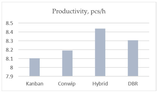
Figure 3.
Comparison of the effectiveness of pull control mechanisms in the process with bottleneck for Cv = 1.25, t = 5min, WIP = 5.
The advantage and novelty of this study is that it is useful as u guideline for many other combinations of levels of independent parameters which are different for different production facilities. This could help managers in this field in making decision on which production control mechanisms to implement.
In practice, lean implementation is not that simple task. There are well known general steps in transforming production processes according to lean principles. Many lean implementation projects start with great success but do not succeed in greater extant, rather slow down or stop due to challenges that emerge. Pull principle is a big challenge for many companies and demands a lot of prerequisites in order to be achieved and that is well described in literature [3,71].
One of the decisions that have to be made when introducing pull in the production is which production control mechanism to use. Effectiveness of pull control mechanisms under various production condition is not the same and for industrial practitioners it is not always clear which control mechanism would be suitable for their process. The process of implementation of pull production mechanisms can be significantly long and to test in real production and then make the decision mechanism to implement is impractical and expensive. Thus, findings gained from this study could help production managers to make decision and choose appropriate pull mechanism.
As was the initial assumption, the results of simulation experimentation showed that the existence of bottleneck in the process affects the efficiency of pull control mechanisms in terms of productivity. That is, one mechanism which is optimal for the process without bottleneck is not optimal for the process with bottleneck. It is also confirmed that for the different level of input parameters, namely variability, process time and number of control cards, different pull control mechanism contribute to better levels of productivity, thus if in the case of a bottleneck one mechanism for one setting of production parameters is optimal for another setting of parameters, also with bottleneck, that same mechanism will not be the best choice.
5. Conclusions
The focus of this study was to explore how the bottleneck influences effectiveness of pull control mechanisms in terms of production productivity in various production conditions, defined by different levels of variability in the production process, processing time and number of signal cards, which actually define the level of work-in-process, since every card is tied to one product at a time. Some previous studies have investigated the influence of bottleneck but not for these production conditions, nor for all of four pull mechanisms researched in this study. In addition, this study gained, regression functions defining the dependence of productivity on all of these mentioned parameters. Regression functions were generated separately for each of the four control mechanisms, and, separately for the process with and the process without the bottleneck. Thus, a total of eight regression functions were generated. The influence of independent parameters, their main effects and interaction effects, on the dependent variable is different in all eight cases, which can be seen by reviewing the regression coefficients shown in Appendix B. This shows that for the same level of parameters the level of productivity will be different depending on the type of control mechanism under consideration. The same goes for the process with or without bottleneck. As shown in more detail in the Discussion section, by calculating the value of productivity, one can make a comparison and decide which control mechanism to choose for implementation. Thus, by knowing the current state of production process in terms of existence of bottleneck, level of variability, processing time and the desired level of work-in process, one can use those regression functions to find determine which pull control mechanism to use in their process. In addition, by knowing the current state of production process regarding bottleneck, variations in the process, level of work in process, industrial practitioners can, by using the knowledge from this study about influence of all these parameters on productivity, make a decision for an improvement goals in the process.
Authors of this study are aware that this type of decision is not a “one-way road”, that is, that many other factors such as previous experience of the company in lean manufacturing in general as a mindset, but also experience in implementing pull principle, can influence the decision which pull control mechanism to use.
The limitation of this study is in that it has considered single-product production, so future studies could focus on researching multiple-product production, as well as different types of production processes other than serial production line explored in this study.
Author Contributions
Conceptualization, N.T. and N.Š.; methodology, N.T.; software, N.T.; validation, N.T. and N.Š.; re-sources, N.T.; writing—original draft preparation, N.T.; writing—review and editing, N.T. and N.Š. All authors have read and agreed to the published version of the manuscript.
Funding
The Article Processing Charges (APCs) is funded by the European Regional Development Fund, grant number KK.01.1.1.07.0052.
Institutional Review Board Statement
Not applicable.
Informed Consent Statement
Not applicable.
Data Availability Statement
Data available on request.
Conflicts of Interest
The authors declare no conflict of interest.
Appendix A
Table A1.
Experiment design table—KANBAN.
Table A1.
Experiment design table—KANBAN.
| Factor 1 | Factor 2 | Factor 3 | Factor 4 | Response 1 | |
|---|---|---|---|---|---|
| Std | A:Coeff. of var. | B:Process. time | C:Bottleneck | D:Num. of Cards | Productivity |
| 79 | 0.25 | 60 | YES | 5 | 0.7358 |
| 61 | 0.25 | 5 | YES | 5 | 8.91 |
| 12 | 0.86 | 60 | NO | 5 | 0.662511 |
| 24 | 0.86 | 60 | YES | 2 | 0.4687 |
| 56 | 0.86 | 60 | YES | 2 | 0.4798 |
| 2 | 0.86 | 5 | NO | 2 | 11.37 |
| 78 | 0.86 | 5 | YES | 5 | 8.4114 |
| 5 | 0.25 | 5 | YES | 2 | 8.89218 |
| 73 | 0.25 | 5 | NO | 5 | 11.9192 |
| 66 | 0.86 | 5 | NO | 2 | 11.391 |
| 47 | 0.25 | 60 | YES | 5 | 0.7261 |
| 51 | 0.25 | 60 | NO | 2 | 0.937762 |
| 75 | 0.25 | 60 | NO | 5 | 0.9615 |
| 54 | 0.86 | 5 | YES | 2 | 8.40368 |
| 22 | 0.86 | 5 | YES | 2 | 8.40368 |
| 69 | 0.25 | 5 | YES | 2 | 8.90216 |
| 14 | 0.86 | 5 | YES | 5 | 8.42742 |
| 43 | 0.25 | 60 | NO | 5 | 0.9594 |
| 67 | 0.25 | 60 | NO | 2 | 0.946778 |
| 32 | 0.86 | 60 | YES | 5 | 0.5497 |
| 44 | 0.86 | 60 | NO | 5 | 0.66613 |
| 1 | 0.25 | 5 | NO | 2 | 11.9043 |
| 6 | 0.86 | 5 | YES | 2 | 8.41359 |
| 68 | 0.86 | 60 | NO | 2 | 0.520305 |
| 23 | 0.25 | 60 | YES | 2 | 0.7266 |
| 21 | 0.25 | 5 | YES | 2 | 8.90216 |
| 25 | 0.25 | 5 | NO | 5 | 11.9262 |
| 35 | 0.25 | 60 | NO | 2 | 0.948248 |
| 46 | 0.86 | 5 | YES | 5 | 8.44544 |
| 42 | 0.86 | 5 | NO | 5 | 11.417 |
| 31 | 0.25 | 60 | YES | 5 | 0.7302 |
| 33 | 0.25 | 5 | NO | 2 | 11.9104 |
| 55 | 0.25 | 60 | YES | 2 | 0.7277 |
| 50 | 0.86 | 5 | NO | 2 | 11.41 |
| 17 | 0.25 | 5 | NO | 2 | 11.9161 |
| 19 | 0.25 | 60 | NO | 2 | 0.945308 |
| 80 | 0.86 | 60 | YES | 5 | 0.5251 |
| 49 | 0.25 | 5 | NO | 2 | 11.9161 |
| 16 | 0.86 | 60 | YES | 5 | 0.4861 |
| 41 | 0.25 | 5 | NO | 5 | 11.9352 |
| 71 | 0.25 | 60 | YES | 2 | 0.7261 |
| 28 | 0.86 | 60 | NO | 5 | 0.568699 |
| 7 | 0.25 | 60 | YES | 2 | 0.7323 |
| 52 | 0.86 | 60 | NO | 2 | 0.525112 |
| 13 | 0.25 | 5 | YES | 5 | 8.9276 |
| 63 | 0.25 | 60 | YES | 5 | 0.74 |
| 15 | 0.25 | 60 | YES | 5 | 0.7277 |
| 65 | 0.25 | 5 | NO | 2 | 11.9181 |
| 18 | 0.86 | 5 | NO | 2 | 11.41 |
| 74 | 0.86 | 5 | NO | 5 | 11.436 |
| 9 | 0.25 | 5 | NO | 5 | 11.9365 |
| 20 | 0.86 | 60 | NO | 2 | 0.537443 |
| 77 | 0.25 | 5 | YES | 5 | 8.9297 |
| 4 | 0.86 | 60 | NO | 2 | 0.539638 |
| 60 | 0.86 | 60 | NO | 5 | 0.605299 |
| 53 | 0.25 | 5 | YES | 2 | 8.91214 |
| 59 | 0.25 | 60 | NO | 5 | 0.962 |
| 3 | 0.25 | 60 | NO | 2 | 0.940212 |
| 64 | 0.86 | 60 | YES | 5 | 0.5425 |
| 72 | 0.86 | 60 | YES | 2 | 0.5113 |
| 37 | 0.25 | 5 | YES | 2 | 8.92212 |
| 62 | 0.86 | 5 | YES | 5 | 8.45244 |
| 76 | 0.86 | 60 | NO | 5 | 0.641898 |
| 48 | 0.86 | 60 | YES | 5 | 0.502 |
| 45 | 0.25 | 5 | YES | 5 | 8.934 |
| 70 | 0.86 | 5 | YES | 2 | 8.43341 |
| 38 | 0.86 | 5 | YES | 2 | 8.45323 |
| 58 | 0.86 | 5 | NO | 5 | 11.465 |
| 11 | 0.25 | 60 | NO | 5 | 0.961 |
| 10 | 0.86 | 5 | NO | 5 | 11.496 |
| 29 | 0.25 | 5 | YES | 5 | 8.937 |
| 40 | 0.86 | 60 | YES | 2 | 0.5225 |
| 39 | 0.25 | 60 | YES | 2 | 0.7246 |
| 34 | 0.86 | 5 | NO | 2 | 11.43 |
| 30 | 0.86 | 5 | YES | 5 | 8.45244 |
| 26 | 0.86 | 5 | NO | 5 | 11.533 |
| 8 | 0.86 | 60 | YES | 2 | 0.5471 |
| 57 | 0.25 | 5 | NO | 5 | 11.9447 |
| 27 | 0.25 | 60 | NO | 5 | 0.9538 |
| 36 | 0.86 | 60 | NO | 2 | 0.551446 |
Std-standard order.
Table A2.
Experiment design table—CONWIP.
Table A2.
Experiment design table—CONWIP.
| Factor 1 | Factor 2 | Factor 3 | Factor 4 | Response 1 | |
|---|---|---|---|---|---|
| Std | A:Coeff. of var. | B:Process. Time | C:Bottleneck | D:Num. of Cards | Productivity |
| 56 | 0.86 | 60 | YES | 2 | 0.5149 |
| 51 | 0.25 | 60 | NO | 2 | 0.9728 |
| 47 | 0.25 | 60 | YES | 3 | 0.7358 |
| 75 | 0.25 | 60 | NO | 3 | 0.971115 |
| 61 | 0.25 | 5 | YES | 3 | 8.935 |
| 64 | 0.86 | 60 | YES | 3 | 0.588179 |
| 24 | 0.86 | 60 | YES | 2 | 0.5251 |
| 3 | 0.25 | 60 | NO | 2 | 0.9656 |
| 18 | 0.86 | 5 | NO | 2 | 11.364 |
| 57 | 0.25 | 5 | NO | 3 | 11.93 |
| 21 | 0.25 | 5 | YES | 2 | 8.974 |
| 17 | 0.25 | 5 | NO | 2 | 11.92 |
| 35 | 0.25 | 60 | NO | 2 | 0.9579 |
| 76 | 0.86 | 60 | NO | 3 | 0.672078 |
| 26 | 0.86 | 5 | NO | 3 | 11.41 |
| 40 | 0.86 | 60 | YES | 2 | 0.5221 |
| 22 | 0.86 | 5 | YES | 2 | 8.48 |
| 31 | 0.25 | 60 | YES | 3 | 0.7261 |
| 78 | 0.86 | 5 | YES | 3 | 8.462 |
| 27 | 0.25 | 60 | NO | 3 | 0.967075 |
| 79 | 0.25 | 60 | YES | 3 | 0.7302 |
| 10 | 0.86 | 5 | NO | 3 | 11.42 |
| 50 | 0.86 | 5 | NO | 2 | 11.326 |
| 16 | 0.86 | 60 | YES | 3 | 0.561857 |
| 11 | 0.25 | 60 | NO | 3 | 0.969696 |
| 25 | 0.25 | 5 | NO | 3 | 11.94 |
| 73 | 0.25 | 5 | NO | 3 | 11.94 |
| 19 | 0.25 | 60 | NO | 2 | 0.959 |
| 55 | 0.25 | 60 | YES | 2 | 0.7354 |
| 29 | 0.25 | 5 | YES | 3 | 8.946 |
| 53 | 0.25 | 5 | YES | 2 | 8.956 |
| 5 | 0.25 | 5 | YES | 2 | 8.943 |
| 6 | 0.86 | 5 | YES | 2 | 8.48 |
| 49 | 0.25 | 5 | NO | 2 | 11.93 |
| 1 | 0.25 | 5 | NO | 2 | 11.937 |
| 74 | 0.86 | 5 | NO | 3 | 11.45 |
| 36 | 0.86 | 60 | NO | 2 | 0.5327 |
| 48 | 0.86 | 60 | YES | 3 | 0.520127 |
| 43 | 0.25 | 60 | NO | 3 | 0.968688 |
| 67 | 0.25 | 60 | NO | 2 | 0.957 |
| 12 | 0.86 | 60 | NO | 3 | 0.67575 |
| 30 | 0.86 | 5 | YES | 3 | 8.503 |
| 68 | 0.86 | 60 | NO | 2 | 0.5376 |
| 4 | 0.86 | 60 | NO | 2 | 0.5503 |
| 54 | 0.86 | 5 | YES | 2 | 8.49 |
| 44 | 0.86 | 60 | NO | 3 | 0.576912 |
| 33 | 0.25 | 5 | NO | 2 | 11.94 |
| 41 | 0.25 | 5 | NO | 3 | 11.94 |
| 60 | 0.86 | 60 | NO | 3 | 0.61404 |
| 52 | 0.86 | 60 | NO | 2 | 0.5525 |
| 63 | 0.25 | 60 | YES | 3 | 0.74 |
| 34 | 0.86 | 5 | NO | 2 | 11.334 |
| 77 | 0.25 | 5 | YES | 3 | 8.927 |
| 39 | 0.25 | 60 | YES | 2 | 0.7262 |
| 14 | 0.86 | 5 | YES | 3 | 8.468 |
| 80 | 0.86 | 60 | YES | 3 | 0.580475 |
| 42 | 0.86 | 5 | NO | 3 | 11.48 |
| 2 | 0.86 | 5 | NO | 2 | 11.364 |
| 62 | 0.86 | 5 | YES | 3 | 8.487 |
| 38 | 0.86 | 5 | YES | 2 | 8.51 |
| 65 | 0.25 | 5 | NO | 2 | 11.937 |
| 23 | 0.25 | 60 | YES | 2 | 0.7303 |
| 8 | 0.86 | 60 | YES | 2 | 0.5154 |
| 69 | 0.25 | 5 | YES | 2 | 8.945 |
| 66 | 0.86 | 5 | NO | 2 | 11.328 |
| 71 | 0.25 | 60 | YES | 2 | 0.7215 |
| 20 | 0.86 | 60 | NO | 2 | 0.5646 |
| 28 | 0.86 | 60 | NO | 3 | 0.651168 |
| 45 | 0.25 | 5 | YES | 3 | 8.925 |
| 59 | 0.25 | 60 | NO | 3 | 0.96143 |
| 7 | 0.25 | 60 | YES | 2 | 0.7277 |
| 32 | 0.86 | 60 | YES | 3 | 0.53714 |
| 13 | 0.25 | 5 | YES | 3 | 8.932 |
| 46 | 0.86 | 5 | YES | 3 | 8.547 |
| 70 | 0.86 | 5 | YES | 2 | 8.59 |
| 9 | 0.25 | 5 | NO | 3 | 11.95 |
| 72 | 0.86 | 60 | YES | 2 | 0.521 |
| 15 | 0.25 | 60 | YES | 3 | 0.7277 |
| 37 | 0.25 | 5 | YES | 2 | 8.959 |
| 58 | 0.86 | 5 | NO | 3 | 11.47 |
Std—standard order.
Table A3.
Experiment design table—Hybrid Kanban/Conwip.
Table A3.
Experiment design table—Hybrid Kanban/Conwip.
| Factor 1 | Factor 2 | Factor 3 | Factor 4 | Response 1 | |
|---|---|---|---|---|---|
| Std | A:Coeff. of var. | B:Process. Time | C:Bottleneck | D:Num. of Cards | Productivity |
| 64 | 0.86 | 60 | YES | 3 | 0.5568 |
| 26 | 0.86 | 5 | NO | 3 | 11.4524 |
| 74 | 0.86 | 5 | NO | 3 | 11.4715 |
| 2 | 0.86 | 5 | NO | 2 | 11.3676 |
| 22 | 0.86 | 5 | YES | 2 | 8.593 |
| 32 | 0.86 | 60 | YES | 3 | 0.5319 |
| 48 | 0.86 | 60 | YES | 3 | 0.4924 |
| 71 | 0.25 | 60 | YES | 2 | 0.7276 |
| 17 | 0.25 | 5 | NO | 2 | 11.9389 |
| 5 | 0.25 | 5 | YES | 2 | 8.9441 |
| 46 | 0.86 | 5 | YES | 3 | 8.552 |
| 30 | 0.86 | 5 | YES | 3 | 8.568 |
| 66 | 0.86 | 5 | NO | 2 | 11.3415 |
| 53 | 0.25 | 5 | YES | 2 | 8.9558 |
| 78 | 0.86 | 5 | YES | 3 | 8.587 |
| 25 | 0.25 | 5 | NO | 3 | 0.7328 |
| 14 | 0.86 | 5 | YES | 3 | 8.594 |
| 44 | 0.86 | 60 | NO | 3 | 0.647 |
| 70 | 0.86 | 5 | YES | 2 | 8.626 |
| 11 | 0.25 | 60 | NO | 3 | 11.977 |
| 79 | 0.25 | 60 | YES | 3 | 8.961 |
| 21 | 0.25 | 5 | YES | 2 | 8.9554 |
| 50 | 0.86 | 5 | NO | 2 | 11.4522 |
| 9 | 0.25 | 5 | NO | 3 | 11.9514 |
| 37 | 0.25 | 5 | YES | 2 | 8.9657 |
| 31 | 0.25 | 60 | YES | 3 | 0.728059 |
| 18 | 0.86 | 5 | NO | 2 | 11.449 |
| 3 | 0.25 | 60 | NO | 2 | 0.9625 |
| 55 | 0.25 | 60 | YES | 2 | 0.7269 |
| 57 | 0.25 | 5 | NO | 3 | 11.9584 |
| 42 | 0.86 | 5 | NO | 3 | 11.5005 |
| 29 | 0.25 | 5 | YES | 3 | 0.9661 |
| 20 | 0.86 | 60 | NO | 2 | 0.5161 |
| 65 | 0.25 | 5 | NO | 2 | 11.9615 |
| 33 | 0.25 | 5 | NO | 2 | 11.947 |
| 16 | 0.86 | 60 | YES | 3 | 0.5495 |
| 15 | 0.25 | 60 | YES | 3 | 0.732221 |
| 10 | 0.86 | 5 | NO | 3 | 11.5316 |
| 68 | 0.86 | 60 | NO | 2 | 0.5209 |
| 8 | 0.86 | 60 | YES | 2 | 0.522 |
| 59 | 0.25 | 60 | NO | 3 | 0.974 |
| 12 | 0.86 | 60 | NO | 3 | 0.6505 |
| 75 | 0.25 | 60 | NO | 3 | 0.9718 |
| 63 | 0.25 | 60 | YES | 3 | 0.742066 |
| 28 | 0.86 | 60 | NO | 3 | 0.6554 |
| 61 | 0.25 | 5 | YES | 3 | 8.934 |
| 39 | 0.25 | 60 | YES | 2 | 0.722 |
| 60 | 0.86 | 60 | NO | 3 | 0.6111 |
| 62 | 0.86 | 5 | YES | 3 | 8.594 |
| 6 | 0.86 | 5 | YES | 2 | 8.5958 |
| 1 | 0.25 | 5 | NO | 2 | 11.923 |
| 23 | 0.25 | 60 | YES | 2 | 0.7256 |
| 36 | 0.86 | 60 | NO | 2 | 0.5331 |
| 7 | 0.25 | 60 | YES | 2 | 0.722 |
| 43 | 0.25 | 60 | NO | 3 | 0.9745 |
| 38 | 0.86 | 5 | YES | 2 | 8.6092 |
| 24 | 0.86 | 60 | YES | 2 | 0.5123 |
| 52 | 0.86 | 60 | NO | 2 | 0.5353 |
| 54 | 0.86 | 5 | YES | 2 | 8.586 |
| 49 | 0.25 | 5 | NO | 2 | 11.9317 |
| 34 | 0.86 | 5 | NO | 2 | 11.4723 |
| 41 | 0.25 | 5 | NO | 3 | 11.9674 |
| 58 | 0.86 | 5 | NO | 3 | 11.5688 |
| 56 | 0.86 | 60 | YES | 2 | 0.5184 |
| 4 | 0.86 | 60 | NO | 2 | 0.547 |
| 19 | 0.25 | 60 | NO | 2 | 0.9656 |
| 69 | 0.25 | 5 | YES | 2 | 8.9757 |
| 72 | 0.86 | 60 | YES | 2 | 0.5077 |
| 80 | 0.86 | 60 | YES | 3 | 0.5085 |
| 77 | 0.25 | 5 | YES | 3 | 8.952 |
| 47 | 0.25 | 60 | YES | 3 | 0.729684 |
| 35 | 0.25 | 60 | NO | 2 | 0.9683 |
| 51 | 0.25 | 60 | NO | 2 | 0.96154 |
| 40 | 0.86 | 60 | YES | 2 | 0.5205 |
| 73 | 0.25 | 5 | NO | 3 | 11.9687 |
| 13 | 0.25 | 5 | YES | 3 | 8.954 |
| 27 | 0.25 | 60 | NO | 3 | 0.9734 |
| 45 | 0.25 | 5 | YES | 3 | 8.958 |
| 76 | 0.86 | 60 | NO | 3 | 0.6269 |
| 67 | 0.25 | 60 | NO | 2 | 0.95691 |
Std—standard order.
Table A4.
Experiment design table—DBR.
Table A4.
Experiment design table—DBR.
| Factor 1 | Factor 2 | Factor 3 | Factor 4 | Response 1 | |
|---|---|---|---|---|---|
| Std | A:Coeff. of var. | B:Process. Time | C:Bottleneck | D:Num. of Cards | Productivity |
| 79 | 0.25 | 60 | YES | 3.5 | 0.747939 |
| 18 | 0.86 | 5 | NO | 2.25 | 11.387 |
| 20 | 0.86 | 60 | NO | 2.25 | 0.6164 |
| 59 | 0.25 | 60 | NO | 3.5 | 0.955385 |
| 32 | 0.86 | 60 | YES | 3.5 | 0.571312 |
| 47 | 0.25 | 60 | YES | 3.5 | 0.75639 |
| 26 | 0.86 | 5 | NO | 3.5 | 11.421 |
| 73 | 0.25 | 5 | NO | 3.5 | 11.937 |
| 23 | 0.25 | 60 | YES | 2.25 | 0.736492 |
| 38 | 0.86 | 5 | YES | 2.25 | 8.595 |
| 55 | 0.25 | 60 | YES | 2.25 | 0.728715 |
| 40 | 0.86 | 60 | YES | 2.25 | 0.5395 |
| 28 | 0.86 | 60 | NO | 3.5 | 0.6 |
| 41 | 0.25 | 5 | NO | 3.5 | 11.931 |
| 9 | 0.25 | 5 | NO | 3.5 | 11.943 |
| 76 | 0.86 | 60 | NO | 3.5 | 0.630769 |
| 27 | 0.25 | 60 | NO | 3.5 | 0.964103 |
| 68 | 0.86 | 60 | NO | 2.25 | 0.5897 |
| 31 | 0.25 | 60 | YES | 3.5 | 0.73579 |
| 58 | 0.86 | 5 | NO | 3.5 | 11.412 |
| 30 | 0.86 | 5 | YES | 3.5 | 8.60618 |
| 36 | 0.86 | 60 | NO | 2.25 | 0.6144 |
| 4 | 0.86 | 60 | NO | 2.25 | 0.6036 |
| 10 | 0.86 | 5 | NO | 3.5 | 11.417 |
| 12 | 0.86 | 60 | NO | 3.5 | 0.577949 |
| 3 | 0.25 | 60 | NO | 2.25 | 0.961 |
| 70 | 0.86 | 5 | YES | 2.25 | 8.608 |
| 64 | 0.86 | 60 | YES | 3.5 | 0.562615 |
| 39 | 0.25 | 60 | YES | 2.25 | 0.731846 |
| 44 | 0.86 | 60 | NO | 3.5 | 0.663077 |
| 24 | 0.86 | 60 | YES | 2.25 | 0.5159 |
| 53 | 0.25 | 5 | YES | 2.25 | 8.987 |
| 19 | 0.25 | 60 | NO | 2.25 | 0.9595 |
| 14 | 0.86 | 5 | YES | 3.5 | 8.60618 |
| 78 | 0.86 | 5 | YES | 3.5 | 8.63924 |
| 72 | 0.86 | 60 | YES | 2.25 | 0.5323 |
| 62 | 0.86 | 5 | YES | 3.5 | 8.6172 |
| 52 | 0.86 | 60 | NO | 2.25 | 0.5856 |
| 49 | 0.25 | 5 | NO | 2.25 | 11.94 |
| 2 | 0.86 | 5 | NO | 2.25 | 11.423 |
| 42 | 0.86 | 5 | NO | 3.5 | 11.388 |
| 57 | 0.25 | 5 | NO | 3.5 | 11.937 |
| 54 | 0.86 | 5 | YES | 2.25 | 8.58 |
| 45 | 0.25 | 5 | YES | 3.5 | 8.95988 |
| 71 | 0.25 | 60 | YES | 2.25 | 0.739623 |
| 37 | 0.25 | 5 | YES | 2.25 | 8.9818 |
| 33 | 0.25 | 5 | NO | 2.25 | 11.96 |
| 66 | 0.86 | 5 | NO | 2.25 | 11.391 |
| 67 | 0.25 | 60 | NO | 2.25 | 0.9615 |
| 69 | 0.25 | 5 | YES | 2.25 | 8.98 |
| 48 | 0.86 | 60 | YES | 3.5 | 0.5512 |
| 22 | 0.86 | 5 | YES | 2.25 | 8.591 |
| 74 | 0.86 | 5 | NO | 3.5 | 11.431 |
| 13 | 0.25 | 5 | YES | 3.5 | 8.97191 |
| 34 | 0.86 | 5 | NO | 2.25 | 11.377 |
| 75 | 0.25 | 60 | NO | 3.5 | 0.963077 |
| 21 | 0.25 | 5 | YES | 2.25 | 8.9708 |
| 43 | 0.25 | 60 | NO | 3.5 | 0.962564 |
| 61 | 0.25 | 5 | YES | 3.5 | 8.97491 |
| 46 | 0.86 | 5 | YES | 3.5 | 8.63423 |
| 50 | 0.86 | 5 | NO | 2.25 | 11.417 |
| 60 | 0.86 | 60 | NO | 3.5 | 0.610256 |
| 11 | 0.25 | 60 | NO | 3.5 | 0.963077 |
| 29 | 0.25 | 5 | YES | 3.5 | 8.9679 |
| 7 | 0.25 | 60 | YES | 2.25 | 0.738613 |
| 17 | 0.25 | 5 | NO | 2.25 | 11.947 |
| 77 | 0.25 | 5 | YES | 3.5 | 8.96189 |
| 63 | 0.25 | 60 | YES | 3.5 | 0.742657 |
| 8 | 0.86 | 60 | YES | 2.25 | 0.5207 |
| 65 | 0.25 | 5 | NO | 2.25 | 11.923 |
| 5 | 0.25 | 5 | YES | 2.25 | 8.976 |
| 16 | 0.86 | 60 | YES | 3.5 | 0.578379 |
| 56 | 0.86 | 60 | YES | 2.25 | 0.5221 |
| 80 | 0.86 | 60 | YES | 3.5 | 0.559897 |
| 15 | 0.25 | 60 | YES | 3.5 | 0.745826 |
| 6 | 0.86 | 5 | YES | 2.25 | 8.6 |
| 51 | 0.25 | 60 | NO | 2.25 | 0.9538 |
| 1 | 0.25 | 5 | NO | 2.25 | 11.931 |
| 25 | 0.25 | 5 | NO | 3.5 | 11.935 |
| 35 | 0.25 | 60 | NO | 2.25 | 0.9738 |
Std—standard order.
Appendix B
Table A5.
Regression coefficient for coded factors.
Table A5.
Regression coefficient for coded factors.
| A | B | C | D | AB | AC | AD | BC | BD | CD | ABC | ABD | ACD | ||
|---|---|---|---|---|---|---|---|---|---|---|---|---|---|---|
| Kanban | 5.44 | −0.195 | −4.74 | −0.7878 | 0.00159 | 0.0485 | 0.0191 | 0.0082 | 0.7152 | - | −0.0087 | 0.0192 | - | −0.0075 |
| (Conwip)0.88 | 4.22 | −0.1465 | −3.49 | −0.5229 | 0.0109 | 0.0174 | 0.0269 | 0.0112 | 0.4574 | 0.0052 | −0.0093 | 0.0132 | - | −0.0067 |
| (Hybrid)0.81 | 3.66 | −0.1195 | −2.91 | −0.414 | 0.0101 | −0.0081 | 0.0246 | 0.0074 | O.3502 | 0.005 | −0.0101 | 0.0112 | 0.0044 | −0.0079 |
| DBR | 5.47 | −0.1806 | −4.76 | −0.7561 | 0.0055 | 0.0437 | 0.0405 | 0.0062 | 0.6848 | - | - | - | - | - |
Table A6.
Regression coefficient for real factors-process with bottleneck.
Table A6.
Regression coefficient for real factors-process with bottleneck.
| Cv | T | Nr | CvT | CvNr | TNr | CvTNr | ||
|---|---|---|---|---|---|---|---|---|
| Kanban | 9.85712 | −0.844392 | −0.150878 | 0.003959 | 0.008078 | 0.001504 | - | - |
| (Conwip)0.88 | 7.6239 | −0.584773 | −0.113088 | −0.025503 | 0.003642 | 0.029719 | 0.000376 | - |
| (Hybrid)0.81 | 6.43031 | −0.231142 | −0.092833 | 0.008571 | −0.002235 | −0.036615 | −0.000215 | 0.001038 |
| DBR | 9.88346 | −0.696599 | −0.151325 | −0.004601 | 0.005583 | 0.016574 | - | - |
Table A7.
Regression coefficient for real factors-process without bottleneck.
Table A7.
Regression coefficient for real factors-process without bottleneck.
| Cv | T | Nr | CvT | CvNr | TNr | CvTNr | ||
|---|---|---|---|---|---|---|---|---|
| Kanban | 13.13354 | −0.936188 | −0.200347 | −0.002739 | 0.003491 | 0.034448 | - | - |
| (Conwip)0.88 | 9.82046 | −0.877525 | −0.144614 | −0.036874 | 0.0051 | 0.117177 | 0.000376 | 0.000376 |
| (Hybrid)0.81 | 8.16982 | −0.563684 | −0.116823 | −0.008266 | −0.004897 | 0.066395 | 0.000215 | 0.001038 |
| DBR | 13.16724 | −0.961586 | −0.201172 | 0.004601 | 0.005583 | 0.016574 |
References
- Tortorella, G.L.; Giglio, R.; van Dun, D.H. Industry 4.0 adoption as a moderator of the impact of lean production practices on operational performance improvement. Int. J. Oper. Prod. Manag. 2019, 39, 860–886. [Google Scholar] [CrossRef]
- Trstenjak, M.; Cajner, H.; Opetuk, T. Industry 4.0 Readiness Factor Calculation: Criteria Evaluation Framework. FME Trans. 2019, 47, 841–845. [Google Scholar] [CrossRef]
- Womack, J.P.; Jones, D.T. Lean Thinking: Banish Waste and Create Wealth in Your Corporation, 2nd ed.; Simon & Schuster: New York, NY, USA, 2003. [Google Scholar]
- Hopp, J.; Spearman, M.L. To Pull or Not to Pull: What Is the Question? Manuf. Serv. Oper. Manag. 2004, 6, 133–148. [Google Scholar] [CrossRef] [Green Version]
- Manikandaprabu, S.; Anbuudayasankar, S.P. Productivity Improvement through Lean. Int. J. Eng. Adv. Technol. 2019, 8, 2657–2660. [Google Scholar]
- Nallusamy, S. Execution of lean and industrial techniques for productivity enhancement in a manufacturing industry. Mater. Today Proc. 2021, 37, 568–575. [Google Scholar] [CrossRef]
- Daneshjo, N.; Malega, P. Measurement of Productivity in Small-Series Production and Application of Lean Production Elements. TEM J. 2020, 9, 107. [Google Scholar]
- Rahani, A.R.; Al-Ashraf, M. Production Flow Analysis through Value Stream Mapping: A Lean Manufacturing Process Case Study. Procedia Eng. 2012, 41, 1727–1734. [Google Scholar] [CrossRef] [Green Version]
- Atul, P.; Pankaj, D. Lean manufacturing as a vital tool for increasing productivity in manufacturing. Mater. Today Proc. 2021, 46, 729–736. [Google Scholar]
- Wang, T.N.; Hung, Y.H. Lean Application: The Design Process and Effectiveness. In Human Systems Engineering and Design II; Springer: Cham, Switzerland, 2020. [Google Scholar] [CrossRef]
- Karrer, C. Engineering Production Control Strategies, a Guide to Tailor Strategies That Unite the Merits of Push and Pull; Springer: Berlin/Heidelberg, Germany, 2012; Chapter 2. [Google Scholar]
- Chu, C.H.; Shih, W.L. Simulation Studies in JIT. Int. J. Prod. Res. 2007, 30, 2573–2586. [Google Scholar] [CrossRef]
- Bonvik, A.M.; Couch, C.; Gershwin, S.B. A Comparison of Production-line Control Mechanisms. Int. J. Prod. Res. 1997, 35, 789–804. [Google Scholar] [CrossRef]
- Bicheno, L. The New Lean Toolbox: Towards Fast Flexible Flow; Picsie Books: Buckingham, UK, 2004. [Google Scholar]
- Goldart, E.M. Theory of Constraints; The North River Press: Great Barrington, MA, USA, 1999. [Google Scholar]
- Altshuler, A.; Anderson, M.; Jones, D.; Roos, D.; Womack, J.P. The Future of the Automobile: The Report of MIT’s International Automobile Program; The MIT Press: Cambridge, MA, USA, 1984. [Google Scholar]
- Womack, J.P.; Jones, D.; Roos, D. The Machine That Changed the World; Simon and Schuster: London, UK, 2007. [Google Scholar]
- Murman, E.; Allen, T.; Bozdogan, K.; Cutcher-Gershenfeld, J.; McManus, H.; Nightingale, D.; Rebentisch, E.; Shields, T.; Stahl, F.; Walton, M.; et al. Lean Enterprise Value: Insights from MIT’s Lean Aerospace Initiative; Palgrave: New York, NY, USA, 2002. [Google Scholar]
- Hines, P.; Holweg, M.; Rich, N. Learning to evolve: A review of contemporary lean thinking. Int. J. Oper. Prod. Manag. 2004, 24, 994–1011. [Google Scholar] [CrossRef] [Green Version]
- de Almeida, J.P.L.; Galina, S.V.R.; Grande, M.M.; Brum, D.G. Lean thinking: Planning and implementation in the public sector. Int. J. Lean Six Sigma 2017, 8, 390–410. [Google Scholar] [CrossRef]
- Jing, S.; Hou, K.; Yan, J.; Ho, Z.-P.; Han, L. Investigating the effect of value stream mapping on procurement effectiveness: A case study. J. Intell. Manuf. 2021, 32, 935–946. [Google Scholar] [CrossRef]
- Qin, Y.; Liu, H. Application of Value Stream Mapping in E-Commerce: A Case Study on an Amazon Retailer. Sustainability 2022, 14, 713. [Google Scholar] [CrossRef]
- Amrani, A.Z.; Garel, B.; Vallespir, B. Lean Transformation in Healthcare: A French Case Study. In Proceedings of the Advances in Production Management Systems: Artificial Intelligence for Sustainable and Resilient Production Systems, APMS 2021, PT II, Nantes, France, 5–9 September 2021. [Google Scholar]
- Antosz, K.; Augustyn, A.; Jasiulewicz-Kaczmarek, M. Application of VSM for Improving the Medical Processes—Case Study. In Advances in Production Management System: Artificial Intelligence for Sustainable and Resilient Production System; APMS 2021; Springer: Berlin/Heidelberg, Germany, 2021. [Google Scholar] [CrossRef]
- Cardoso, W. Stream mapping as lean healthcare’s tool to see wastage and improvement points: The case of the emergency care management of a university hospital. Rev. Gest. Sist. Saúde São Paulo 2020, 9, 360–380. [Google Scholar] [CrossRef]
- Yu, T.; Demirli, K.; Bhuiyan, N. Lean transformation framework for treatment-oriented outpatient departments. Int. J. Prod. Res. 2021, 1–15. [Google Scholar] [CrossRef]
- Lima, R.M.; Dinis-Carvalho, J.; Souza, T.; Vieira, E.; Gonçalves, B. Implementation of Lean in Healthcare environments: An update of systematic reviews. Int. J. Lean Six Sigma 2020, 12, 399–431. [Google Scholar] [CrossRef]
- Muiambo, C.C.E.; Joao, I.M.; Navas, H.V.G. Lean waste assessment in a laboratory for training chemical analysts for the pharmaceutical industry. Int. J. Lean Six Sigma 2021. [Google Scholar] [CrossRef]
- Byrne, B.; McDermott, O.; Noonan, J. Applying Lean Six Sigma Methodology to a Pharmaceutical Manufacturing Facility: A Case Study. Processes 2021, 9, 550. [Google Scholar] [CrossRef]
- Gaspar, F.; Fabiano, L. A methodology for applying the shop floor management method for sustaining lean manufacturing tools and philosophies: A study of an automotive company in Brazil. Int. J. Lean Six Sigma 2020, 11, 1219–1238. [Google Scholar] [CrossRef]
- Singh, J.; Singh, H. Application of lean manufacturing in automotive manufacturing unit. Int. J. Lean Six Sigma 2020, 11, 171–210. [Google Scholar] [CrossRef]
- Furman, J.; Malysa, T. The use of lean manufacturing (LM) tools in the field of production organization in the metallurgical industry. Metalurgija 2021, 60, 431–433. [Google Scholar]
- Reyes, S.; Jeampiere, A.; Castro, S.; Fernanda, R. Application of Lean Techniques to Reduce Preparation Times: Case Study of a Peruvian Plastic Company. Int. J. Appl. Eng. Res. 2017, 12, 13541–13551. [Google Scholar]
- De La Vega, M.; Baez-Lopez, Y.; Limon-Romero, J.; Tlapa, D.; Flores, D.L.; Borbón, M.I.R.; Maldonado-Macías, A.A. Lean Manufacturing Critical Success Factors for the Transportation Equipment Manufacturing Industry in Mexico. IEEW Access 2020, 8, 168534–168545. [Google Scholar] [CrossRef]
- Zahraee, M. A survey on lean manufacturing implementation in the selected manufacturing industry in Iran. Int. J. Lean Six Sigma 2016, 7, 136–148. [Google Scholar] [CrossRef]
- Zakaria, D.; Zoubeir, L.; Marc, B. Application of Lean to the Bidding Phase in Building Construction: A French contractors’ Experience. Int. J. Lean Six Sigma 2017, 8, 153–180. [Google Scholar]
- Awad, T.; Guardiola, J.; Fraíz, D. Sustainable Construction:Improving Productivity through Lean Construction. Sustainability 2021, 13, 13877. [Google Scholar] [CrossRef]
- Gjeldum, N.; Veža, I.; Bilić, B. Simulation of Production Process reorganized with Value Stream Mapping. Tech. Gaz. 2011, 18, 341–347. [Google Scholar]
- Lai, E.T.H.; Yun, F.N.J.; Arokiam, I.C.; Joo, J.H.A. Barriers Affecting Successful Lean Implementation in Singapore’s Shipbuilding Industry: A Case Study. Oper. Supply Chain Manag. Int. J. 2020, 13, 166–175. [Google Scholar] [CrossRef]
- Amitkumar, D.M.; Gajanan, S.P. A methodical literature review on application of Lean & Six Sigma in various industries. Aust. J. Mech. Eng. 2019, 19, 107–121. [Google Scholar] [CrossRef]
- Spearman, M.L.; Woodruff, D.L.; Hopp, W.J. CONWIP: A Pull Alternative to Kanban. Int. J. Prod. Res. 1990, 28, 879–894. [Google Scholar] [CrossRef]
- Enns, S.T. Pull replenishment performance as a function of demand rates and setup times under optimal settings. In Proceedings of the 2007 Winter Simulation Conference, Washington, DC, USA, 9–12 December 2007; Institute of Electrical and Electronics Engineers: Piscataway, NJ, USA, 2007; pp. 1624–1632. [Google Scholar]
- Yang, L.; Zhang, X.P. Design and Application of Kanban Control System in a Multi-Stage, Mixed-Model Assembly Line. Syst. Eng. Theory Pract. 2009, 29, 64–72. [Google Scholar] [CrossRef]
- Lavoie, P.; Gharbi, A.; Kenne, J.P. A comparative study of pull control mechanisms for unreliable homogenous transfer lines. Int. J. Prod. Econ. 2010, 124, 241–251. [Google Scholar] [CrossRef]
- Pettersen, J.A. Pull Based Production Systems—Performance, Modeling and Analysis. Ph.D. Thesis, Lulea University of Technology, Lulea, Sweden, 2010. [Google Scholar]
- Pettersen, J.A.; Segerstedt, A. Restricted work-in-process: A study of differences between Kanban and CONWIP. Int. J. Prod. Econ. 2009, 118, 199–207. [Google Scholar] [CrossRef]
- Sharma, S.; Agrawal, N. Selection of a pull production control policy under different demand situations for a manufacturing system by AHP-algorithm. Comput. Oper. Res. 2009, 36, 1622–1632. [Google Scholar] [CrossRef]
- Yang, T.; Hung, Y.H.; Huang, K.C. A simulation study on CONWIP System Design for Bicycle Chain Manufacturing. In Proceedings of the 9th IFAC Conference on Manufacturing Modelling, Management, and Control (MIM 2019), Berlin, Germany, 28–30 August 2019; IFAC-PapersOnLine. Volume 52. [Google Scholar]
- Leonardo, D.G.; Sereno, B.; da Silva, D.S.A.; Sampaio, M.; Massote, A.A.; Simões, J.C. Implementation of hybrid Kanban-CONWIP system: A case study. J. Manuf. Technol. Manag. 2017, 28, 714–736. [Google Scholar] [CrossRef]
- Stevenson, S.; Found, P. Completely Taktless! What Is Pull in the Context of the Process Industries? In Understanding the Lean Enterprise; Springer: Cham, Switzerland, 2016; pp. 153–184. [Google Scholar]
- Gayer, B.D.; Saurin, T.A.; Wachs, P. A method for assessing pull production systems: A study of manufacturing, healthcare, and construction. Prod. Plan. Control 2021, 32, 1063–1083. [Google Scholar] [CrossRef]
- Aldas, D.; Reyes, J.P.; Aman, R.J. Manufacturing Strategies for an optimal pull-type production control system. Case study in a textile industry. In Proceedings of the 4th International Congress of Innovation and Trends in Engineering (CONIITI) 2018, Bogota, Colombia, 3–5 October 2018. [Google Scholar]
- Piplani, R.; Ang, A.W.H. Performance comparison of multiple product Kanban control systems. Int. J. Prod. Res. 2018, 56, 1299–1312. [Google Scholar] [CrossRef]
- Hopp, W.J.; Spearman, M.C. Factory Physics, 3rd ed.; Waveland Press Inc.: Long Grove, IL, USA, 2008. [Google Scholar]
- Boonlertvanich, K. Extended CONWIP-Kanban System: Control and Performance. Ph.D. Thesis, Georgia Institute of Technology, SAD, Atlant, GA, USA, 2005. [Google Scholar]
- Sokolowski, J.A.; Banks, C.M. Principles of Modeling and Simulation; John Wiley & Sons, Inc.: Hoboken, NJ, USA, 2009. [Google Scholar]
- Law, A.M.; Kelton, W.D. Simulation Modeling and Analysis, 2nd ed.; McGraw-Hill: New York, NY, USA, 1991. [Google Scholar]
- Terrence, M.J. A Simulation and Evaluation Study of the Economic Production Quantity Lot Size and Kanban for Single Line, Multi–Product Production System Under Various Setup Times. Ph.D. Thesis, Kent State University, SAD, Kent, OH, USA, 2008. [Google Scholar]
- Darlingtona, J.; Francisb, M.; Foundc, P.; Thomasc, A. Design and implementation of a Drum-Buffer-Rope pull-system. Prod. Plan. Control 2015, 26, 489–504. [Google Scholar] [CrossRef]
- Marek, R.P.; Elkins, D.A.; Smith, D.R. Understanding the fundamentals of Kanban and CONWIP pull systems using simulation. In Proceedings of the Winter Simulation Conference 2001, Arlington, VA, USA, 9–12 December 2001. [Google Scholar]
- Enns, S.T.; Rogers, P. Clarifying CONWIP versus PUSH system behavior using simulation. In Proceedings of the 2008 Winter Simulation Conference, Miami, FL, USA, 7–10 December 2008; Mason, S.J., Hill, R.R., Mönch, L., Rose, O., Jefferson, T., Fowler, J.W., Eds.; Institute of Electrical and Electronics Engineers: Piscataway, NJ, USA, 2008; pp. 1867–1872. [Google Scholar]
- Sandanayake, Y.G.; Oduoza, C.F.; Proverbs, D.G. A systematic modelling and simulation approach for JIT performance optimization. Robot. Comput.-Integr. Manuf. 2008, 24, 735–743. [Google Scholar] [CrossRef]
- Suri, R. Quick Response Manufacturing. A Company Approach to Reducing Lead Times; Productivity Press: New York, NY, USA, 1998. [Google Scholar]
- Sergent, R.G. Verification and validation of simulation models. In Proceedings of the 2010 Winter Simulation Conference, Baltimore, MD, USA, 5–8 December 2010. [Google Scholar]
- Prakash, J.; Chin, J.F. A comparison of push and pull production controls under machine breakdown. Int. J. Bus. Sci. Appl. Manag. 2011, 6, 58–70. [Google Scholar]
- Omer, F.B.; Serpil, E. Simulation modelling and analysis of a JIT production system. Int. J. Prod. Econ. 1998, 55, 203–212. [Google Scholar]
- Matlab R2017b. Available online: https://www.mathworks.com/products/simevents/whatsnew.html (accessed on 17 November 2017).
- Myers, R.H.; Montgomery, D.C.; Anderson-Cook, C.M. Response Surface Methodology: Process and Product Optimization Using Designed Experiments, 3rd ed.; Wiley: New York, NY, USA, 2009. [Google Scholar]
- Design-Expert® Software Version 11. Available online: https://www.statease.com/dx11.html (accessed on 14 November 2017).
- Cajner, H.; Tonković, Z.; Šakić, N. The significance of data transformation in analysis of experiments. In Proceedings of the 12th International Scientific Conference on Production Engineering, CIM 2009, Biograd, Croatia, 17–20 June 2009; Eberhard, A., Toma, U., Damir, C., Eds.; Croatian Association of Production Engineering: Zagreb, Croatia, 2009. [Google Scholar]
- Monden, Y. Toyota Production System: An Integrated Approach to Just-In-Time, 4th ed.; Taylor & Francis Group: Abingdon, UK, 2012. [Google Scholar]

Publisher’s Note: MDPI stays neutral with regard to jurisdictional claims in published maps and institutional affiliations. |
© 2022 by the authors. Licensee MDPI, Basel, Switzerland. This article is an open access article distributed under the terms and conditions of the Creative Commons Attribution (CC BY) license (https://creativecommons.org/licenses/by/4.0/).