An Adapted Two-Steps Approach to Simulate Nonlinear Vibrations of Solid Undergoing Large Deformation in Contact with Rigid Plane—Application to a Grooved Cylinder

Abstract

Simulating the full dynamic response of a rolling sculpted tire requires not only taking into account various non-linearities but also considering the multi-scale nature of the dynamic response itself. On one hand, there is the macroscopic rolling dynamic behavior that operates around the rotating frequency with relatively high amplitudes. On the other hand, the vibratory response operates in a larger frequency window with relatively low amplitudes. In contrast to a straightforward strategy that consists of using an energy-conserving stable time integrator to predict the multi-scale dynamic response, the proposed strategy is based on a two-steps approach to separate the dynamics operating at different scales. This methodology is applied to simulate the nonlinear vibrations of a hyperelastic solid undergoing large deformations in contact with a rigid plane. In order to illustrate the potential of the proposed numerical method, the nonlinear vibrations response of a grooved cylinder rolling on a rigid plane is investigated.

1. Introduction

Tire/road noise is becoming a major source of vehicle noise as the transition towards electrical vehicles is underway. This has resulted in tire manufacturers refining their tire design to help reduce traffic noise. The basic physical principles of tire/pavement noise are well understood and documented [1]. For the interested reader, a literature review of design considerations on parameters influencing tire/pavement interaction noise can be found in [2] and a complete review of models on tire–pavement interaction noise is also provided in [3]. The tire/pavement noise generation mechanisms can be divided into two categories. The first one is an air-flow mechanism that generates noise at high frequencies (above 1000 Hz) and is commonly referred to as air-pumping. The second one is the tire vibrations mechanism that generates noise at low and medium frequencies (below 1000 Hz). These noise generation mechanisms are well described in [4]. This paper focuses on the latter mechanism.

The tire solid vibrations are generated by two excitation sources. The first one is the road roughness for which the resulting vibrations could be well predicted for axi-symmetric tires using an ALE-formulation [5,6]. This approach consists of using a fixed mesh through which the tire material particles flow. This approach gives a stationary state of the loaded rotating tire. Afterward, the small vibrations due to the road excitation could be computed using a modal superposition technique [7,8]. Most industrial models found in the literature are based on this approach. The second excitation source is the tire’s groove resonance. The small scale tread deformation has an impact on the noise emitted by the tire [9]. The main goal of the grooves is to ensure sufficient grip in wet conditions in order to avoid hydroplaning; however, the tire groove geometry parameters (length, width, angle, depth…) and the material proprieties change the vibratory behavior of the tire [10,11]. The prediction of the vibrations induced by this second mechanism can be more complex to achieve and requires the implementation of a specific methodology. Indeed, obtaining a stationary state is no longer possible and full Lagrangian vision should be adopted to treat the tire’s large deformations. Hence, a time integration process seems unavoidable. The vibrations small scale requires using energy conserving schemes [12,13] but remains costly from a CPU time perspective.

The main contribution of the proposed study is to promote a numerical methodology based on a two-step approach for solving such problem [14]. Firstly, a non-linear quasi-static simulation is performed to avoid using a high-order stable numerical scheme capable of handling the considered non-linearities. Afterward, the non-stationary equations of motion are linearized using the quasi-static response as a reference point. The method was originally proposed by Valyaev [15] for linear elastic materials. The effectiveness of the proposed approach is illustrated by predicting the non-linear vibrations of a grooved cylinder rolling on a rigid plane with frictionless contact in the first case and with frictional contact in the second case. Even if special attention is given to the mechanical contact, since the tire vibration noise is mainly caused by the impact between the tire and the pavement [4], the main objective is not to propose a reality of the physical phenomena and the interaction between the vibratory response of the tire and the road, but only to demonstrate the capacity of the numerical methodology put forward to correctly predict the vibratory response of solid undergoing large deformation with frictional contact.

This paper is organized as follows. Section 2 presents the mathematical framework used to describe the mechanical behavior of a hyperelastic solid undergoing large deformations in contact with a rigid plane. Afterward, the linearization process is detailed and several hypotheses are made and justified. The efficiency of the proposed strategy is demonstrated by applying it to simulate the non-linear vibrations of a grooved cylinder. The prototype structure and the numerical results are presented in Section 3. Finally, the concluding remarks are given in Section 4.

2. Problem Setting

This section sets the mathematical framework used to develop the proposed methodology. Firstly, the mechanical quantities needed to use the large deformation theory are introduced. Afterward, the mathematical formulation of the frictional contact is presented. Then, the equations of motion are given with the corresponding weak formulations. Finally, the perturbation of the quasi-static simulation that gives the vibration response is detailed.

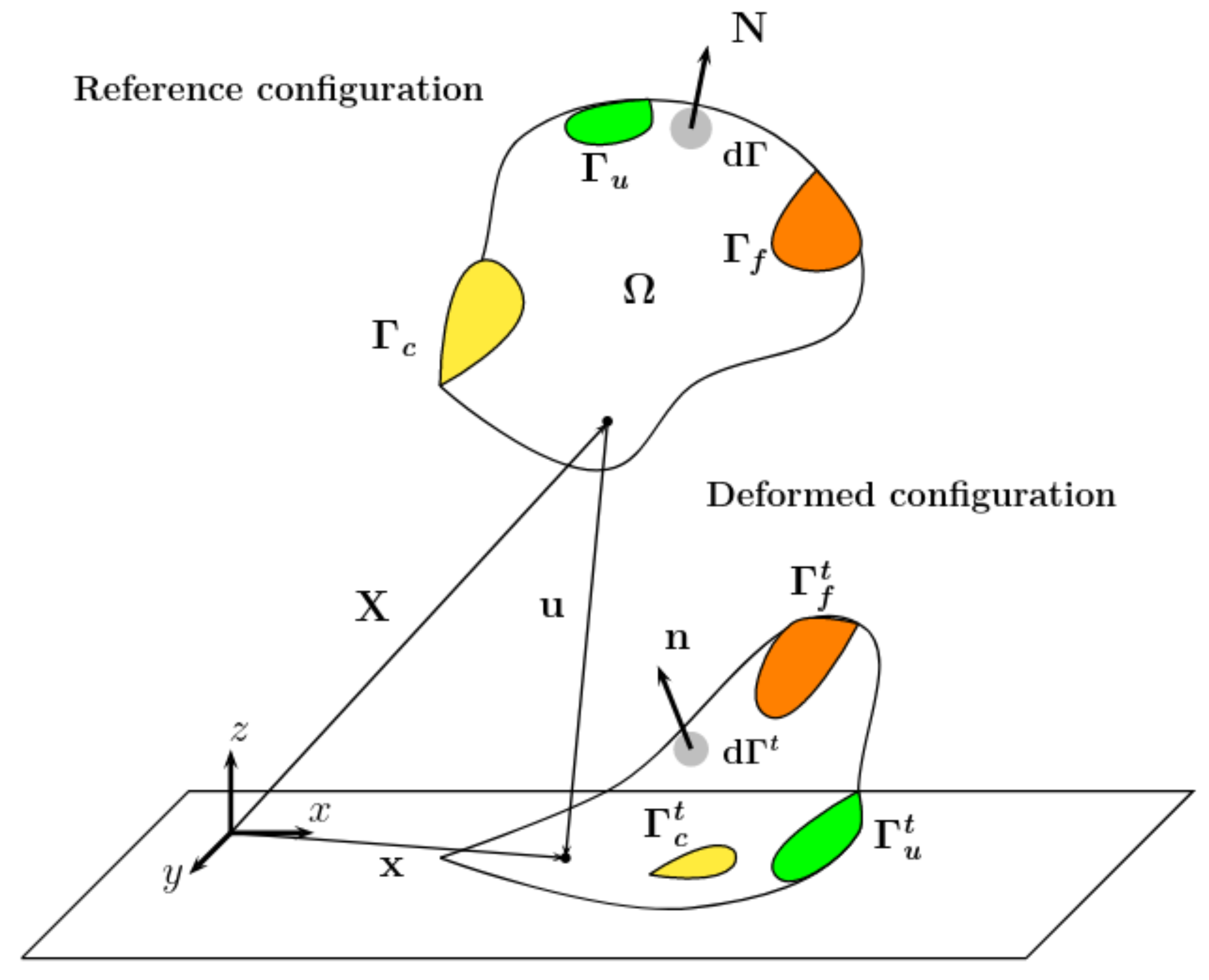
2.1. Notations

An open set $\Omega \subset {\mathbb{R}}^3$ represents the reference state of a continuum body with material points $\mathbf{X}\in \Omega$, $\mathbf{x}=\mathbf{\phi }(\mathbf{X},t)\in {\mathbb{R}}^3$ is the deformation field of the body relative to its reference state at time $t\in [0,+\infty ]$ and $\mathbf{u}(\mathbf{X},t)=\mathbf{x}-\mathbf{X}$ is the displacement field. The boundary of the material domain $\partial \Omega$ is composed of ${\Gamma }_u$ where the displacement is imposed, ${\Gamma }_f$ where the external force is imposed and ${\Gamma }_c$ the potential contact zone.

The gradient of a quantity in the reference configuration is noted ∇. To describe the deformation, several mechanical quantities are introduced. The identity matrix is denoted by $\mathbf{I}$ and the deformation gradient is represented by $\mathbf{F}=\mathbf{I}+\nabla \mathbf{u}$. The Jacobian of φ is denoted by $J=det\left(\mathbf{F}\right)$. $\mathbf{C}={\mathbf{F}}^{⊺}\mathbf{F}$ represents the Cauchy–Green tensor and $\mathbf{E}=\frac{1}{2}(\mathbf{C}-\mathbf{I})$ is the Green–Lagrange strain tensor. $\sigma$ is the Cauchy stress tensor, $\mathbf{P}=J\sigma {\mathbf{F}}^{-⊺}$ is the first Piola–Kirchhoff stress tensor and $\mathbf{S}=J{\mathbf{F}}^{-1}\sigma {\mathbf{F}}^{-⊺}$ is the second Piola–Kirchhoff stress tensor. To treat rubber-like materials, a general hyperelastic constitutive law is considered. This law is derived from the strain energy function W that depends on the deformation through E [16]. The second Piola–Kirchhoff stress tensor is given by:

$$\mathbf{S}=\frac{\partial W}{\partial \mathbf{E}}\left(\mathbf{E}\right)$$

(1)

with corresponding fourth-order elasticity tensor

$$\mathcal{C}=\frac{\partial \mathbf{S}}{\partial \mathbf{E}}=\frac{{\partial }^{2}W}{\partial \mathbf{E}\partial \mathbf{E}}$$

(2)

The fourth-order material elasticity tensor $\mathcal{C}$ is necessary within typical finite element procedures and is used in the linearization procedure later on.

2.2. Contact Mechanics

A unilateral contact with rigid plane is considered, as illustrated in Figure 1. ${\Gamma }_c$ is a restricted part of $\partial \Omega$ and represents the surface where contact/friction phenomena may occur. $\mathbf{N}$ (resp. $\mathbf{n}$) is the unit outward normal in the reference (resp. current) configuration. The motion of the body is restricted to the upper half-space $z\ge 0$ from the rigid plane $z=0$.

To treat the geometrical non linearity, the equilibrium equations are written in the reference configuration. Thus, the second definition of the force will be privileged. The traction vector is decomposed in the deformed configuration as follows:

$$\mathbf{PN}={\Pi }_n\mathbf{n}+{\Pi }_t$$

(3)

where ${\Pi }_n\mathbf{n}$ is the normal stress vector and ${\Pi }_t$ is the tangential stress vector at the interface. ${\Pi }_t$ is calculated as follows:

$${\Pi }_t=(\mathbf{I}-\mathbf{n}\otimes \mathbf{n})·\mathbf{PN}$$

(4)

The contact constraint’s mathematical formulation requires also the displacement field decomposition in the contact patch

$$\mathbf{u}=u_n\mathbf{n}+{\mathbf{u}}_t$$

(5)

where $u_n$ (resp. ${\mathbf{u}}_t$) is the normal (resp. tangential) displacement.

2.2.1. Signorini Conditions

The non-penetration condition in the contact surface is mathematically formulated using the normal gap function $g_n$ defined as:

$$g_n=-\mathbf{x}.\mathbf{n}\ge 0$$

(6)

The gap function could be written using the displacement $\mathbf{u}$

$$\begin{array}{cc}\hfill g_n\left(\mathbf{u}\right)=& -(\mathbf{X}+\mathbf{u}).\mathbf{n}\hfill \\ \hfill =& g_0-u_n\hfill \end{array}$$

(7)

where $g_0>0$ is the initial gap. To prevent the body from penetrating the plane, a non-positive contact pressure arises in the contact zone.

$${\Pi }_n\le 0$$

(8)

Finally, if a point is not in contact, then ${\Pi }_n=0$, meanwhile ${\Pi }_n<0$ if not. This leads to the non-penetration non-adhesion condition:

$${\Pi }_n{g}_n=0$$

(9)

The force acting on an element of area in the deformed configuration is defined via

$$df=\sigma \mathbf{n}\mathrm{d}{\Gamma }^t=\mathbf{PN}\mathrm{d}\Gamma$$

(10)

The set of the presented conditions are called Hertz–Signorini–Morea or Karush–Kuhn–Tucker conditions [17]:

$$g_n\ge 0,{\Pi }_n\le 0,g_n{\Pi }_n=0\mathrm{on}{\Gamma }_c$$

(11)

These conditions provide the basis to treat frictionless contact problems in the context of constraint optimization.

2.2.2. Coulomb Friction Law

Friction on the contact interface can be introduced in the general form [18]:

$${\Pi }_t={\Pi }_t({\Pi }_n,{\dot{\Pi }}_n,{\dot{\mathbf{u}}}_t,t,\dots )$$

(12)

The simplest friction law states that the tangential resistance of the contact interface depends on the contact pressure and that the direction of the tangential stress vector is given by the sliding direction $\mathbf{s}$.

$${\Pi }_t={\Pi }_t({\Pi }_n,\mathbf{s})\mathrm{where}\mathbf{s}=\left\{\begin{array}{cc}\hfill \frac{{\dot{\mathbf{u}}}_t}{\Vert {\dot{\mathbf{u}}}_t\Vert }\hfill & \hfill \mathrm{if}\Vert {\dot{\mathbf{u}}}_t\Vert >\mathbf{0}\hfill \\ \hfill \mathbf{0}\hfill & \hfill \mathrm{if}\Vert {\dot{\mathbf{u}}}_t\Vert =\mathbf{0}\hfill \end{array}\right.$$

(13)

where ${\dot{\mathbf{u}}}_t$ is the sliding velocity. The relative motion of the point along the rigid plane is confined by the frictional shear force in the way that the point remains at the initial contact location if the shear stress vector is smaller than the critical frictional stress ${\Pi }_t^c$, which in Coulomb’s friction law is proportional to the contact pressure, so the point does not move if

$$\Vert {\Pi }_t\Vert \le {\Pi }_t^c=\mu \left|{\Pi }_n\right|$$

(14)

where the coefficient of proportionality $\mu$ is the coefficient of friction. The maximal permitted tangential stress in equilibrium straight motion is limited by $\mu |{\Pi }_n|$. The contact condition in the slip regime is

$${\Pi }_t-\mu \left|{\Pi }_n\right|\mathbf{s}=\mathbf{0}$$

(15)

The former condition could be generalized to the stick regime by multiplying it by the norm of the sliding velocity $\Vert {\dot{\mathbf{u}}}_t\Vert$

$$\Vert {\dot{\mathbf{u}}}_t\Vert {\Pi }_t-\mu \left|{\Pi }_n\right|{\dot{\mathbf{u}}}_t=\mathbf{0}$$

(16)

A complementary condition is added to distinguish stick and slip states

$$\Vert \mathbf{s}\Vert \Vert {\Pi }_t-\mu \left|{\Pi }_n\right|\mathbf{s}\Vert =0$$

(17)

Union of all fore mentioned conditions forms the set of conditions for Coulomb’s friction law

$$\Vert {\Pi }_t\Vert \le \mu |{\Pi }_n|,\Vert {\dot{\mathbf{u}}}_t\Vert {\Pi }_t-\mu \left|{\Pi }_n\right|{\dot{\mathbf{u}}}_t=0,\Vert \mathbf{s}\Vert \Vert {\Pi }_t-\mu \left|{\Pi }_n\right|\mathbf{s}\Vert =0\mathrm{on}{\Gamma }_c$$

(18)

The Coulomb’s friction law is sufficient to describe the macroscopic dry friction treated in this paper. For the interested reader, more complex friction laws based on tribological considerations at contact interfaces could be found in [19].

2.3. Equations of Motion

The contact conditions together with the relevant boundary conditions complement the local balance of momentum and angular momentum ($\sigma ={\sigma }^{⊺}$). The inertia effects are neglected and a quasi-static process will be considered to deal with Coulomb friction. Hence, the equations of motion are written as follows:

$$\begin{array}{c}\hfill \left\{\begin{array}{cc}\nabla ·\mathbf{P}+\mathbf{f}=\mathbf{0}\hfill & \hfill \mathrm{in}\Omega \hfill \\ \mathbf{P}\mathbf{N}={\mathbf{F}}_0\hfill & \hfill \mathrm{on}{\Gamma }_f\hfill \\ \mathbf{u}={\mathbf{u}}_d\hfill & \hfill \mathrm{on}{\Gamma }_u\hfill \\ g_n\ge 0,{\Pi }_n\le 0,g_n{\Pi }_n=0\hfill & \hfill \mathrm{on}{\Gamma }_c\hfill \\ \Vert {\Pi }_t\Vert \le \mu |{\Pi }_n|,\Vert {\dot{\mathbf{u}}}_t\Vert {\Pi }_t-\mu \left|{\Pi }_n\right|{\dot{\mathbf{u}}}_t=0,\Vert \mathbf{s}\Vert \Vert {\Pi }_t-\mu \left|{\Pi }_n\right|\mathbf{s}\Vert =0\hfill & \hfill \mathrm{on}{\Gamma }_c\hfill \end{array}\right.\end{array}$$

(19)

$\mathbf{f}$ defines the volume external forces, ${\mathbf{F}}_0$ is a prescribed traction (Neumann boundary conditions) and ${\mathbf{u}}_d$ is a prescribed displacement (Dirichlet boundary conditions).

In order to obtain the weak formulation, which is the starting point of the finite element method, the first equation of (19) is multiplied by a test function $\mathbf{v}$ and integration by parts is then performed. The weak formulation is stated as follows:

Find $\mathbf{u}\in \mathcal{U}=\left\{\mathbf{u}\in H^1(\Omega )|\mathbf{u}={\mathbf{u}}_{d}on{\Gamma }_u\right\}$

$$\begin{array}{c}\hfill {\int }_{\Omega }\mathbf{P}:\nabla \mathbf{v}\mathrm{d}\Omega -{\int }_{\Omega }\mathbf{f}.\mathbf{v}\mathrm{d}\Omega -{\int }_{\partial \Omega }\mathbf{P}\mathbf{N}.\mathbf{v}\mathrm{d}\Gamma =0\forall \mathbf{v}\in \mathcal{V}\end{array}$$

(20)

where $\mathcal{V}=\left\{\mathbf{u}\in H^1(\Omega )|\mathbf{u}=\mathbf{0}on{\Gamma }_u\right\}$. The integral defined on the boundary are separated as follows:

$${\int }_{\partial \Omega }\mathbf{PN}.\mathbf{v}\mathrm{d}\Gamma ={\int }_{{\Gamma }_f}{\mathbf{F}}_0.\mathbf{v}\mathrm{d}\Gamma +{\int }_{{\Gamma }_c}\mathbf{PN}.\mathbf{v}\mathrm{d}\Gamma$$

(21)

The first term takes into account the Neumann boundary condition. The second one is related to the contact constraint and could be written as follows

$$\begin{array}{cc}\hfill {\int }_{{\Gamma }_c}\mathbf{P}\mathbf{N}.\mathbf{v}\mathrm{d}\Gamma =& {\int }_{{\Gamma }_c}({\Pi }_n\mathbf{n}+{\Pi }_t).(v_n\mathbf{n}+{\mathbf{v}}_{\mathbf{t}})\mathrm{d}\Gamma \hfill \\ \hfill =& {\int }_{{\Gamma }_c}({\Pi }_n{v}_n+{\Pi }_t.{\mathbf{v}}_{\mathbf{t}})\mathrm{d}\Gamma \hfill \end{array}$$

(22)

The weak formulation could now be written as follows:

$$\begin{array}{c}\hfill \left\{\begin{array}{c}\mathrm{Find}\mathbf{u}\in \mathcal{U}\hfill \\ {\int }_{\Omega }\mathbf{P}:\nabla \mathbf{v}\mathrm{d}\Omega -{\int }_{\Omega }\mathbf{f}.\mathbf{v}\mathrm{d}\Omega -{\int }_{{\Gamma }_f}{\mathbf{F}}_0.\mathbf{v}\mathrm{d}\Gamma ={\int }_{{\Gamma }_c}{\Pi }_n{v}_n+{\Pi }_t.{\mathbf{v}}_{\mathbf{t}}\mathrm{d}\Gamma \forall \mathbf{v}\in \mathcal{V}\hfill \\ g_n\ge 0,{\Pi }_n\le 0,g_n{\Pi }_n=0\hfill & \hfill \mathrm{on}{\Gamma }_c\hfill \\ \Vert {\Pi }_t\Vert \le \mu |{\Pi }_n|\Vert {\dot{\mathbf{u}}}_t\Vert {\Pi }_t-\mu \left|{\Pi }_n\right|{\dot{\mathbf{u}}}_t=0\Vert \mathbf{s}\Vert \Vert {\Pi }_t-\mu \left|{\Pi }_n\right|\mathbf{s}\Vert =0\hfill & \hfill \mathrm{on}{\Gamma }_c\hfill \end{array}\right.\end{array}$$

(23)

Several formulations can be applied to incorporate the contact constraints into the variational formulation. Most standard finite element codes that are able to handle contact problems use either the penalty or the Lagrange multiplier method. Each of the methods has its own advantages and disadvantages. The methods are designed to fulfill the constraint equations in the normal direction in the contact interface. For the tangential part, a constitutive relation is needed when stick/slip motion occurs [19].

The penalty method is used to treat the normal contact condition. An active set strategy is employed to obtain the active contact zone. The normal contact condition contribution to the weak formulation is approximated as follows [20].

$${\int }_{{\Gamma }_c}{\Pi }_n{v}_n\mathrm{d}\Gamma ={\int }_{{\Gamma }_c}{\epsilon }_n{g}_n^{-}\left(\mathbf{u}\right)v_n\mathrm{d}\Gamma$$

(24)

where ${\epsilon }_n$ is the normal penalty parameter and $g_n^{-}=min(g_n,0)$ is the penetration function. As ${\epsilon }_n\to \infty$, the gap function $g_n\to 0$ on ${\Gamma }_c$, the constraint is increasingly well-satisfied. However, large values of ${\epsilon }_n$ will lead to an ill-conditioned numerical problem.

The Coulomb friction law is regularized using a linear approximation in the stick regime. The tangential contact contribution to the weak formulation is written as in [21]:

$${\int }_{{\Gamma }_c}{\Pi }_t.{\mathbf{v}}_{\mathbf{t}}\mathrm{d}\Gamma ={\int }_{{\Gamma }_c}\mu \left|{\Pi }_n\right|\left\{\begin{array}{cc}\frac{1}{{\epsilon }_r}(2-\frac{\Vert {\dot{\mathbf{u}}}_t\Vert }{{\epsilon }_r}){\dot{\mathbf{u}}}_{\mathbf{t}}.{\mathbf{v}}_{\mathbf{t}}\mathrm{d}\Gamma \hfill & \mathrm{if}\Vert {\dot{\mathbf{u}}}_{\mathbf{t}}\Vert <{\epsilon }_r\hfill \\ \frac{1}{\Vert {\dot{\mathbf{u}}}_{\mathbf{t}}\Vert }{\dot{\mathbf{u}}}_{\mathbf{t}}.{\mathbf{v}}_{\mathbf{t}}\mathrm{d}\Gamma \hfill & \mathrm{if}\Vert {\dot{\mathbf{u}}}_{\mathbf{t}}\Vert \ge {\epsilon }_r\hfill \end{array}\right.$$

(25)

where ${\epsilon }_r$ is the regularization coefficient. It determines the boundary between the stick and the slip regime. If ${\epsilon }_r\to 0$, we obtain the classical Coulomb law. Since the problem is written in a quasi-static framework, the sliding velocity ${\dot{\mathbf{u}}}_{\mathbf{t}}$ is approximated using a finite difference method. The analytical contribution of each integral term to the tangent matrix and to the nonlinear residual could be found in [21].

2.4. Dynamic Response

The weak formulation is solved using finite element method. Afterward, the quasi-static response is used to linearize the dynamic response. Several hypotheses are made and explained and the linearization process is detailed.

2.4.1. Main Hypothesis

The quasi-static problem, as formulated in the former section, is given by:

$$\begin{array}{c}\hfill {\int }_{\Omega }{\mathbf{P}}_{\mathbf{1}}:\nabla \mathbf{v}\mathrm{d}\Omega -{\int }_{\Omega }\mathbf{f}.\mathbf{v}\mathrm{d}\Omega -{\int }_{{\Gamma }_f}{\mathbf{F}}_0.\mathbf{v}\mathrm{d}\Gamma ={\mathbf{R}}_c\left({\mathbf{u}}_{\mathbf{1}}\right)\forall \mathbf{v}\in \mathcal{V}\end{array}$$

(26)

where ${\mathbf{R}}_c$ is the virtual work of the contact forces. The virtual work due to the inertial forces is added to the weak formulation. The dynamic problem is given by:

$$\begin{array}{c}\hfill {\int }_{\Omega }\rho {\ddot{\mathbf{u}}}_{\mathbf{2}}.\mathbf{v}\mathrm{d}\Omega +{\int }_{\Omega }{\mathbf{P}}_{\mathbf{2}}:\nabla \mathbf{v}\mathrm{d}\Omega -{\int }_{\Omega }\mathbf{f}.\mathbf{v}\mathrm{d}\Omega -{\int }_{{\Gamma }_f}{\mathbf{F}}_0.\mathbf{v}\mathrm{d}\Gamma ={\mathbf{R}}_c({\mathbf{u}}_{\mathbf{2}},{\dot{\mathbf{u}}}_{\mathbf{2}})\forall \mathbf{v}\in \mathcal{V}\end{array}$$

(27)

where $\rho$ is the density. The dynamic response ${\mathbf{u}}_{\mathbf{2}}$ is supposedly the sum of the quasi-static response ${\mathbf{u}}_{\mathbf{1}}$ and the vibrations field $\mathbf{w}$. In other words, the inertia effects are only considered for the vibrations problem.

$${\mathbf{u}}_{\mathbf{2}}(\mathbf{X},t)={\mathbf{u}}_{\mathbf{1}}(\mathbf{X},t)+\mathbf{w}(\mathbf{X},t)+o\left(\mathbf{w}\right)$$

(28)

An homogeneous Dirichlet boundary condition is applied on ${\Gamma }_u$ since the prescribed displacement is the same for both problems.

$$\mathbf{w}=\mathbf{0}\mathrm{on}{\Gamma }_u$$

(29)

The active contact zone ${\Gamma }_c^t$ and the virtual work of the contact forces are supposedly the same for the dynamic and quasi-static problem.

$${\mathbf{R}}_c({\mathbf{u}}_{\mathbf{2}},{\dot{\mathbf{u}}}_{\mathbf{2}})\approx {\mathbf{R}}_c\left({\mathbf{u}}_{\mathbf{1}}\right)$$

(30)

The active contact zone is not exactly the same since the inertia terms will change the contact stiffness and thus alter the contact patch [22]. Another difference between the virtual works is the friction law formulation. The sliding velocity is approximated in the quasi-steady regime whereas it is equal to the tangent velocity in the dynamic regime.

Given the hypothesis that the inertia effect does not change the contact patch, the normal displacement in the quasi-steady regime does not change in the dynamic regime since it is determined by the rigid plane position. Therefore, the normal vibrations field is null on the contact active zone.

$$\mathbf{w}.\mathbf{n}=0\mathrm{on}{\Gamma }_c^t$$

(31)

This boundary condition is an interpretation of the contact constraint as a Dirichlet-like boundary condition. The active contact zone ${\Gamma }_c^t$ is not related to a material domain, which is problematic from a mathematical point view; however, it is easily implemented after a finite element discretization.

2.4.2. Linearization

The linearization process starts with expressing the mechanical quantities of the dynamic problem as function of the mechanical quantities of the quasi-static problem with neglecting high order terms

$$\begin{array}{cc}\hfill {\mathbf{F}}_{\mathbf{2}}& ={\mathbf{F}}_{\mathbf{1}}+\nabla \mathbf{w}\hfill \\ \hfill {\mathbf{E}}_{\mathbf{2}}& ={\mathbf{E}}_{\mathbf{1}}+\frac{1}{2}({{\mathbf{F}}_{\mathbf{1}}}^{⊺}\nabla \mathbf{w}+{\nabla }^{⊺}\mathbf{w}{\mathbf{F}}_{\mathbf{1}}+\underset{\approx \mathbf{0}}{\underbrace{{\nabla }^{⊺}\mathbf{w}\nabla \mathbf{w}}})\hfill \\ \hfill & \approx {\mathbf{E}}_{\mathbf{1}}+\frac{1}{2}(\nabla \mathbf{w}+{\nabla }^{⊺}\mathbf{w}+{\nabla }^{⊺}{\mathbf{u}}_{\mathbf{1}}\nabla \mathbf{w}+{\nabla }^{⊺}\mathbf{w}\nabla {\mathbf{u}}_{\mathbf{1}})\hfill \\ \hfill & \approx {\mathbf{E}}_{\mathbf{1}}+{\mathbf{E}}_{\mathbf{w},{\mathbf{u}}_{\mathbf{1}}}\hfill \end{array}$$

(32)

The constitutive material law is linearized as follows

$$\begin{array}{cc}\hfill {\mathbf{S}}_{\mathbf{2}}& =\frac{\partial W}{\partial \mathbf{E}}\left({\mathbf{E}}_2\right)=\frac{\partial W}{\partial \mathbf{E}}({\mathbf{E}}_1+{\mathbf{E}}_{\mathbf{w},{\mathbf{u}}_{\mathbf{1}}})\hfill \\ \hfill & \approx \frac{\partial W}{\partial \mathbf{E}}\left({\mathbf{E}}_1\right)+\frac{{\partial }^{2}W}{\partial \mathbf{E}\partial \mathbf{E}}\left({\mathbf{E}}_{\mathbf{1}}\right):{\mathbf{E}}_{\mathbf{w},{\mathbf{u}}_{\mathbf{1}}}\hfill \\ \hfill & \approx {\mathbf{S}}_1+{\mathcal{C}}_1:{\mathbf{E}}_{\mathbf{w},{\mathbf{u}}_{\mathbf{1}}}\hfill \end{array}$$

(33)

The deformation integral term is linearized as follows

$$\begin{array}{cc}\hfill {\mathbf{P}}_{\mathbf{2}}:\nabla \mathbf{v}& ={\mathbf{S}}_{\mathbf{2}}:({\mathbf{F}}_{\mathbf{2}}^{⊺}\nabla \mathbf{v})\hfill \\ \hfill & =({\mathbf{S}}_{\mathbf{1}}+{\mathcal{C}}_{\mathbf{1}}:{\mathbf{E}}_{\mathbf{w},{\mathbf{u}}_{\mathbf{1}}}):({\mathbf{F}}_{\mathbf{1}}^{⊺}\nabla \mathbf{v}+{\nabla }^{⊺}\mathbf{w}\nabla \mathbf{v})\hfill \\ \hfill & ={\mathbf{P}}_{\mathbf{1}}:\nabla \mathbf{v}+{\mathbf{S}}_{\mathbf{1}}:{\nabla }^{⊺}\mathbf{w}\nabla \mathbf{v}+({\mathcal{C}}_1:{\mathbf{E}}_{\mathbf{w},{\mathbf{u}}_{\mathbf{1}}}):({\mathbf{F}}_{\mathbf{1}}^{⊺}\nabla \mathbf{v})\hfill \end{array}$$

(34)

The weak formulation governing the vibrations response is given by

$$\begin{array}{c}\hfill {\int }_{\Omega }\rho \ddot{\mathbf{w}}.\mathbf{v}\mathrm{d}\Omega +{\int }_{\Omega }{\mathbf{S}}_{\mathbf{1}}:{\nabla }^{⊺}\mathbf{w}\nabla \mathbf{v}+({\mathcal{C}}_1:{\mathbf{E}}_{\mathbf{w},{\mathbf{u}}_{\mathbf{1}}}):({\mathbf{F}}_{\mathbf{1}}^{⊺}\nabla \mathbf{v})\mathrm{d}\Omega =-{\int }_{\Omega }\rho {\ddot{\mathbf{u}}}_{\mathbf{1}}.\mathbf{v}\mathrm{d}\Omega \forall \mathbf{v}\in \mathcal{V}\end{array}$$

(35)

The deformation integral term depends on the gradient of the quasi-static displacement. The quasi-steady acceleration ${\ddot{\mathbf{u}}}_{\mathbf{1}}$ appears as the excitation force. It is approximated using a finite difference scheme. The second derivative numerical approximation generates high frequency noise. It could be handled by using low-pass filter or by choosing an adequate discretization. Equation (35) is linear with respect to $\mathbf{w}$ and could be solved using a time integration scheme.

3. Numerical Results

In this section, a numerical example intended to demonstrate the utility and performance of the proposed method is presented. The quasi-static problem is solved using a finite element code called MEF++, which is developed by the GIREF of Laval University (Groupe Interdisciplinaire de Recherche en Éléments Finis). The studied prototype is presented and the simulation numerical parameters are given. Afterward, the quasi-static simulation results are analyzed. Finally, the vibrations field is extracted using the presented method. The coefficient of friction impact on the quasi-static problem and on the vibrations is investigated.

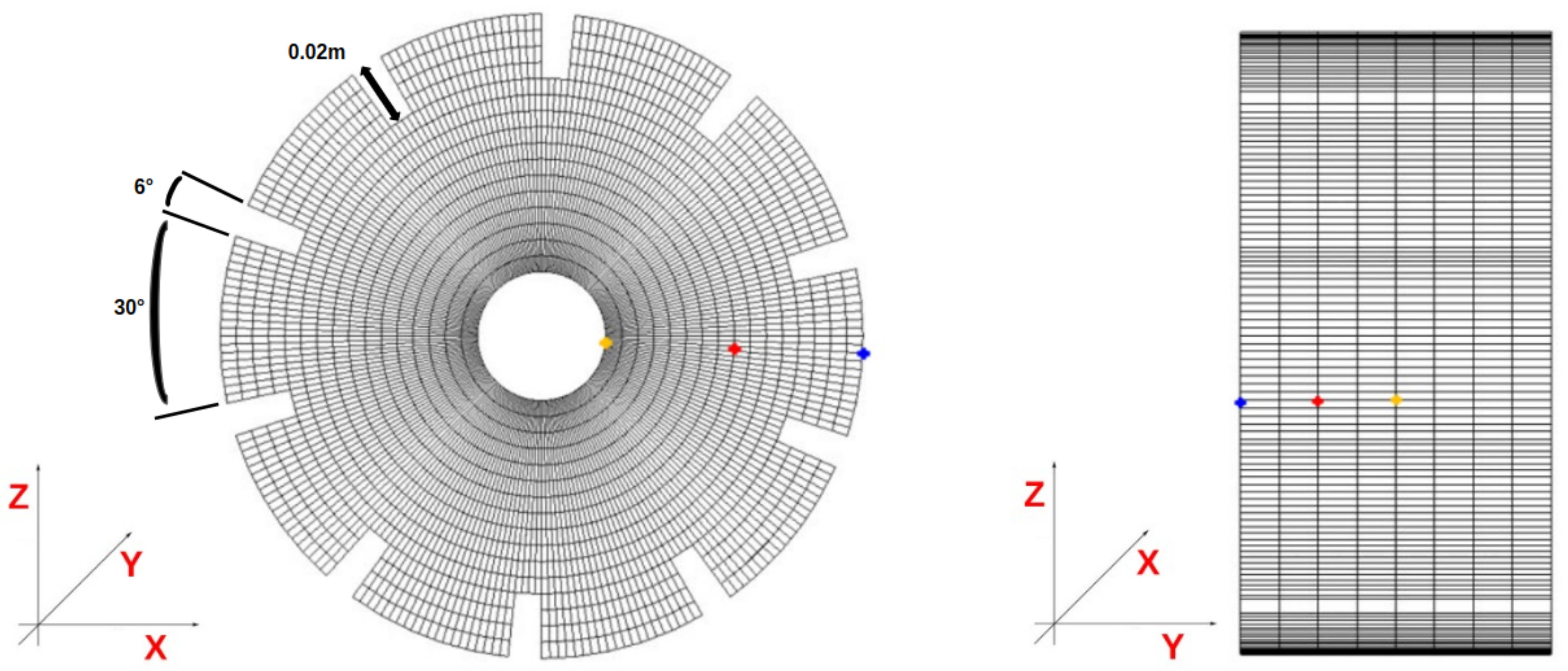
3.1. Prototype

The method presented in the former section is applied to predict the dynamic response of the grooved cylinder shown in Figure 2. The cylinder is composed of 10 blocks. The chosen mesh is a result of a convergence study with respect to the quasi-static displacement and the contact forces. The mesh is composed of 35,640 nodes and 29,440 linear elements.

The material domain is composed of the potential contact surface (in red) ${\Gamma }_c$ and the rim zone ${\Gamma }_u$ (in blue) where the following Dirichlet boundary condition is applied:

$$\mathbf{u}(\mathbf{X},t)={[Vt0-d]}^{⊺}+\mathbf{R}\left(\omega t\right)\mathbf{X}-\mathbf{X}\mathrm{in}{\Gamma }_u$$

(36)

The structure is loaded kinematically by applying a vertical displacement d in the rim zone. The load could be thus calculated by summing the vertical reactions in the contact patch. V is the translation velocity, and $\mathbf{R}$ is the rotation matrix associated with the angular velocity $\omega$. The translation velocity depends on the angular velocity via the effective radius (also known as the rolling radius) $r_{\omega }=V/\omega$. A first order approximation of $r_{\omega }$ is given as a function of the geometrical radius $R_e$ (see [23] for more details) as follows

$$r_{\omega }\approx R_e-\frac{d}{3}$$

(37)

The tire rubber is commonly modeled by using an hyperelastic material constitutive law. The simplest hyperelastic material model is the Saint Venant–Kirchhoff model, which is just an extension of the geometrically linear elastic material model to the geometrically nonlinear regime.

$$\mathbf{S}=\lambda \mathrm{tr}\left(\mathbf{E}\right)\mathbf{I}+2\mu \mathbf{E}$$

(38)

where $\lambda$ and $\mu$ are the Lamé constants. The numerical results presented in the next section are obtained using the geometrical and the material constitutive law properties given in

Table 1. Prototype mechanical properties.

External radius	${\mathit{R}}_{\mathit{e}}=0.1$ m
Internal radius	$R_i=0.02$ m
Width	$w=0.1$ m
Young Modulus	$E=2\times {10}^8$ Pa
Poisson coefficient	$\nu =0.3$
Density	$\rho =900$ kg/m3

. The rolling conditions and the simulation numerical parameters are also given in

Table 2. Simulation parameters.

Deflection	$\mathit{d}=0.01$ m
Rotation speed	$\omega =150$ rad/s
Normal penalization	${\epsilon }_n={10}^{12}$
Regularization coefficient	${\epsilon }_r={10}^{-6}$
Time step	$\Delta t={10}^{-4}$ s

. The chosen parameters are the result of a preliminary convergence study that is not presented. In fact, the resulting quasi-static displacement is practically invariant with respect to higher values of ${\epsilon }_n$ and lower values of ${\epsilon }_r$ using the chosen mesh and the mechanical properties given in Table 1.

3.2. Quasi-Static Rolling

The quasi-static rolling results are now presented. In order to study the deformation of the structure, the displacement field is extracted for different points as shown in Figure 3.

The first selection provides insight into the displacement variation in the radial direction while the second one provides an insight into the displacement variation in the lateral direction.

3.2.1. Preample-Frictionless Contact

The analysis of the quasi-static rolling is initiated by considering a frictionless contact. Although this first case studied, based on frictionless contact, does not make sense for the reality of tire-road interaction, as it does not correspond to the real phenomena of tire contact, this preliminary study is carried out only to illustrate the feasibility and validity of the proposed two-steps approach on the grooved cylinder under study. In addition, this first application with frictionless contact will serve as a reference for a qualitative comparison with the following case, which considers the impact of friction. So the main objective of this section is to study the kinematics and the contact pressure of the grooved cylinder in order to validate both the mechanical modeling and the associated numerical methodology.

Figure 4 shows the time evolution of the quasi-static displacement components. The displacement field is, as expected, periodic. The longitudinal displacement $U_{\mathrm{x}}$ slows down at the entry of the contact patch $(t\approx$ 0.05 s) and speeds up at the exit of the contact patch $(t\approx$ 0.055 s) to reach the rim longitudinal position. The longitudinal deformation decreases as we move away from the contact zone. The same kinematical behavior is observed for tires in [23]. In fact, the radial distance between the tread pattern and the rotation axis is minimal at the contact patch and reach its maximum at the opposite of the contact patch. The vertical displacement $U_{\mathrm{z}}$ shows that the non-penetration condition is well respected $(0.05$ s $\le t\le 0.055$ s) on the contact patch. The lateral displacement amplitude $U_{\mathrm{y}}$ decreased as we move away from the contact patch due to the Poisson effect. The lateral deformation is obviously greater in the contact active zone and is null at the opposite of the contact patch $(t\approx 0.07$ s). Furthermore, the lateral displacement has a symmetric distribution; the deformation at the entry of the contact zone is the same at the exit of the contact patch and the maximum is reached at the contact patch center $(t\approx 0.052$ s). The displacement of the node occupying the rim zone shows that the Dirichlet boundary conditions are well respected.

Figure 5 shows that the lateral position does not impact the longitudinal and vertical displacement. The lateral displacement amplitude decreases toward 0 as we move to the contact patch center. This result was expected since the plane $(y=0)$ is a symmetry plane of the structure.

Equation (35) shows that the quasi-steady acceleration appears as the excitation force of the vibrations response. The acceleration evolution in the circumferential direction and in the frequency domain is displayed in order to have an idea on how the vibrations will be excited.

Figure 6 shows the time evolution of the acceleration in the rotating frame. The angle $\theta =0$ deg denotes the contact patch center and $\theta <0$ deg designates the contact patch exit. From a time perspective, the acceleration’s maximum is reached when the block edge enters $(t\approx 0.052$ s) and leaves $(t\approx 0.0563$ s) the contact patch. From a circumferential point of view, the maximum of the vertical and lateral acceleration is located at the contact patch boundaries and have a similar distribution at the entry $(\theta \approx 20\mathrm{deg})$ and at the exit $(\theta \approx -17\mathrm{deg})$ of the contact active zone. The vertical acceleration is null in the contact zone since the vertical displacement is constant in the contact patch. The lateral acceleration decreases towards 0 as we move away from the contact patch. The longitudinal acceleration has a shear distribution in the contact patch. An acceleration at the entry of the contact patch and a deceleration at the exit patch are observed. The balance between the acceleration and the deceleration varies with respect to the contact patch form.

Figure 7 shows the associated quasi-steady acceleration spectrum plotted with respect to the order. The order is defined as the frequency over the rotation speed and it is used to analyze the spectrum distribution independently of the rotation frequency. The fundamental frequency is equal to the rotation frequency $(\mathrm{Order}=1)$. Two families of harmonics appear since various non-linearities are taken into account in the model. The first family of harmonics operates around the multiples of the rotation frequency $n\omega ,n\in \mathbb{N}$. The second family of harmonics operates around 10 k$\omega ,k\in \mathbb{N}$, with a modulation effect. It concerns the contact forces frequency since the structure is composed of 10 blocks. This modulation phenomena is due to the rotation effect [24,25]. In fact, the kinematical quantities are calculated with respect to the fixed frame while the contact forces are connected to the rotating frame. This phenomena is not observed in the lateral direction since it represents the rotation axis direction. The vertical and longitudinal accelerations have the same order of magnitude, which is greater than the one of the lateral acceleration. Finally, the acceleration amplitude decreases as we move away from the contact patch.

Figure 8 shows the contact pressure distribution with respect to the position of the groove (leading and trailing edge). When a block enters the contact zone, the contact pressure is concentrated at the entry. As the block advances, the contact pressure moves to the block center and becomes similar to the distribution of the cylindrical contact pressure described in Hertz theory [26]. As the block exits the contact patch, the pressure becomes concentrated in the trailing edge with the same distribution as the one observed for the leading edge. A small variation of the total contact force is observed. Since the deflection d is constant and the contact patch form is changing, the load supported by the structure varies. The last figure shows the spectrum of the total force variation $\delta F_z$, which represents the difference between the total contact force and its mean value. It shows that the variation spectrum is composed of harmonics located around the multiples of the blocks frequency. In the following, the Coulomb friction law is now considered and its impact on the quasi-static rolling is investigated.

3.2.2. Extension by Considering the Impact of the Friction Coefficient

The Coulomb friction is now taken into account using the regularization method presented in Section 2. The friction coefficient impact on the quasi-static rolling is investigated.

Figure 9 shows the displacement evolution in the contact zone for various values of $\mu$. We observe that increasing $\mu$ favors the stick regime. The longitudinal displacement remains constant for $\mu \ge 0.3$ and the lateral displacement variation decreases as the coefficient of friction increases. Indeed, the tangential pressure needed to switch to the slip regime increases knowing that the structure is subjected to the same deflection. The lateral displacement maximum has moved towards the exit of the contact patch when the friction is added. Furthermore, the lateral displacement at the entry of the contact patch is no longer similar to the one at the exit of the contact patch. The vertical displacement is more or less the same since the friction is mainly acting on the tangential components.

Figure 10 shows the normal contact pressure distribution at different stages of the contact. Similar to the frictionless contact, the contact pressure maximum is located at the entrance (resp. exit) for the the nodes located at the entry (resp. exit) of the block. Unlike the frictionless case, the distribution at the exit is different than the distribution at the entry since the friction law is characterized by a time-dependent path and the mechanical system is no longer conservative. Increasing $\mu$ leads also to the saturation of the normal contact pressure.

Figure 11 shows the tangential contact pressure is increasing with respect to $\mu$ unlike the normal contact pressure where a saturation effect is noticed. The tangential contact pressure has the same evolution as the normal pressure for the nodes located at the middle of the block $\theta ={\theta }_c$ and at the exit of the block $\theta ={\theta }_s$; however, an increase in the norm of the tangential pressure of the leading edge at the exit of the contact patch is observed. The differences observed between the tangential pressure for various values of $\mu$ is explained by the change of the slope in the stick regime and the change of the tangential pressure value in the slip regime.

Figure 12 shows the total contact force variation. As for the frictionless case, the total lateral force $F_y$ is null since the plane $(y=0)$ is a symmetry plane of the structure. The variation of the vertical load is a little bit greater as the coefficient of friction $\mu$ increases until reaching an invariant evolution. In fact, $F_z$ remains the same for $\mu =(0.3-0.5-1.0)$. This is coherent with the saturation phenomena observed for the normal contact pressure. The total longitudinal contact force amplitude decreases as we increase $\mu$. High frequency oscillations appear for larger values of $\mu$. These oscillations represent a consequence of the tangent pressure variation described in Figure 11.

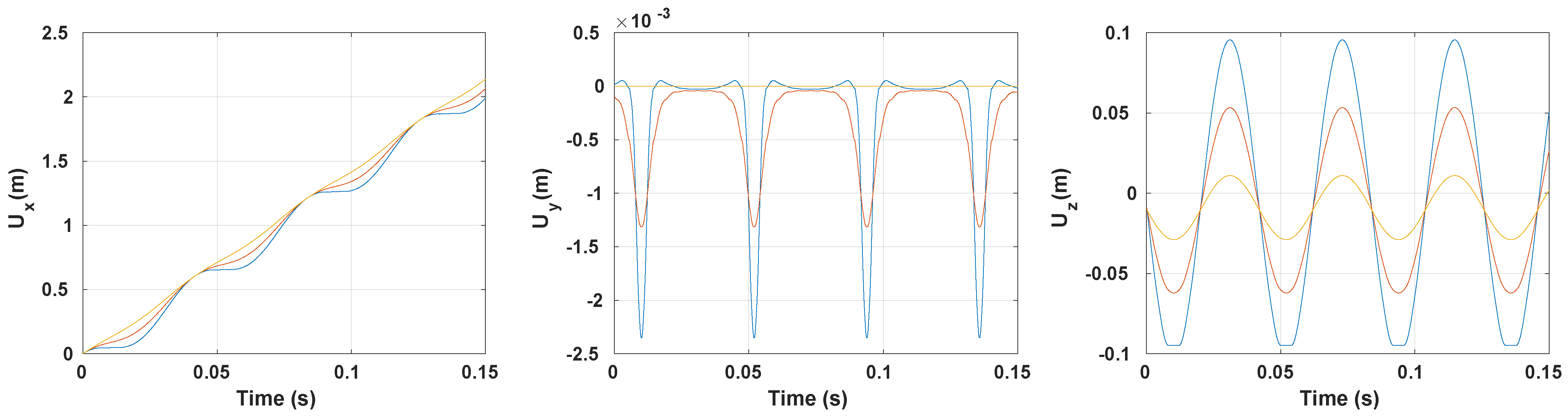
3.3. Vibration Response

The linearization method is used to calculate the vibrations field. The vibrations problem is solved using a time integration technique via an implicit Euler scheme. Since the prototype has a relatively simple geometry and constitutive material law, the dynamic problem could also be solved using the same integration scheme. The validity of the linearization process is then verified. Afterward, the coefficient of friction influence on the vibratory response is investigated.

3.3.1. Preample-Frictionless Contact

As for the quasi-static rolling, a frictionless contact is considered first. As a reminder, this first preliminary study based on the prediction of the nonlinear vibration response with frictionless contact only aims to illustrate the feasibility of the proposed two-steps approach. A comparison between the linearization method solution and the reference solution, which represents the difference between the dynamic and the quasi-static response is presented. Then, the vibrations velocity spectrum is analyzed. Finally, the vibrations spatial evolution is visualized to assess the global vibration behavior of the grooved cylinder.

Figure 13 illustrates the comparison between the linearized solution and the reference solution. Both solutions are, as expected, periodic. Both solutions have the same vibration frequency with a small difference with respect to the phase. The vertical vibrations are null in the contact patch for both methods; therefore, treating the normal contact constraint as a Dirichlet-like boundary condition seems to be the right choice. The longitudinal vibrations maximum amplitude is located in the contact patch and have the same order of magnitude as the vertical vibrations. The lateral vibrations are located in the contact zone and decrease towards 0 as we move away from the contact zone. The magnitude of the lateral vibrations are much lower than the vertical and longitudinal components.

Figure 14 shows the vibrations velocity spectrum. Both solutions give more or less the same vertical and longitudinal velocities. The main difference between the methods are observed in the lateral direction. A set harmonics around the multiples of the blocks frequency with the same modulation effect described in the quasi-static rolling results is observed for both solutions. The lateral vibrations velocity spectrum has a frequency comb distribution. The harmonics around the multiples of the rotation frequency have vanished for the longitudinal and vertical vibrations. Hence, the linearization method allows us to separate the dynamic behaviors operating at different scales. The vertical and longitudinal vibration velocity magnitude is more or less the same and greater than the magnitude of the lateral velocity. The same observation was found for the quasi-steady acceleration.

Figure 15 illustrates the vibrations variation in the radial and lateral directions. The vibrations amplitude decreases as we move away from the tread pattern in the radial direction. The lateral vibrations amplitude decreases as we move towards the contact center in the lateral direction whereas the vertical and longitudinal vibrations remain constant. The same observation was found for the quasi-static displacement in Figure 4 and Figure 5.

Figure 16 shows the vibrations velocity variation in the circumferential direction. Unlike the quasi-steady acceleration, the mechanical behavior at the entry of the contact patch is no longer similar to the behavior at the exit of the contact patch. The vertical vibrations are, as expected, null in the contact patch and at the opposite of the contact patch ($\theta =180$ deg). The lateral vibrations maximum is situated at the contact patch entry and decreases towards 0 as we move away from the contact active zone. The longitudinal vibrations velocity has a more or less symmetric distribution with respect to the plane $(z=R_i)$.

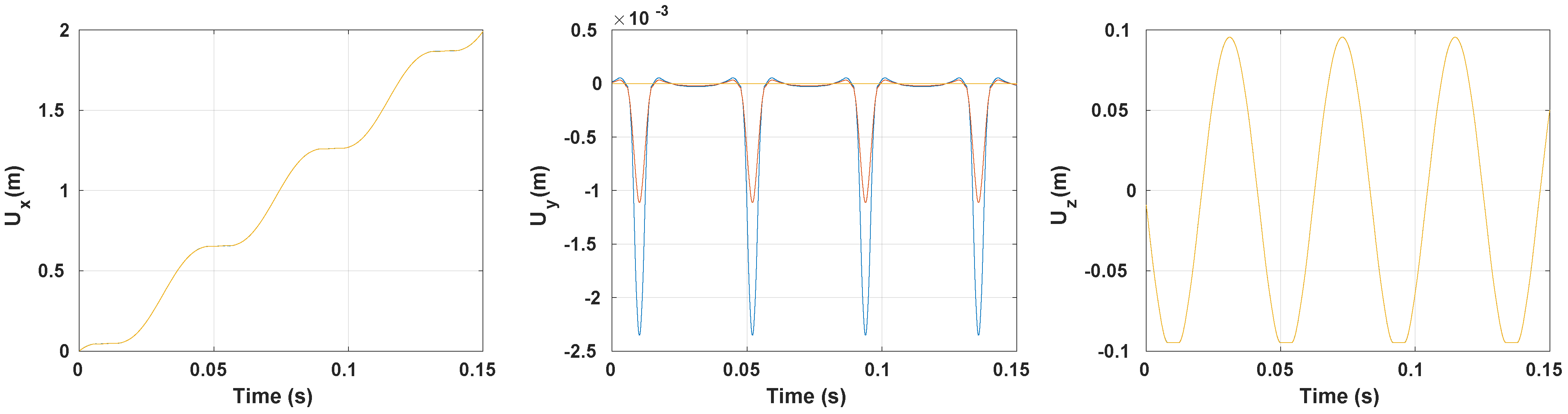
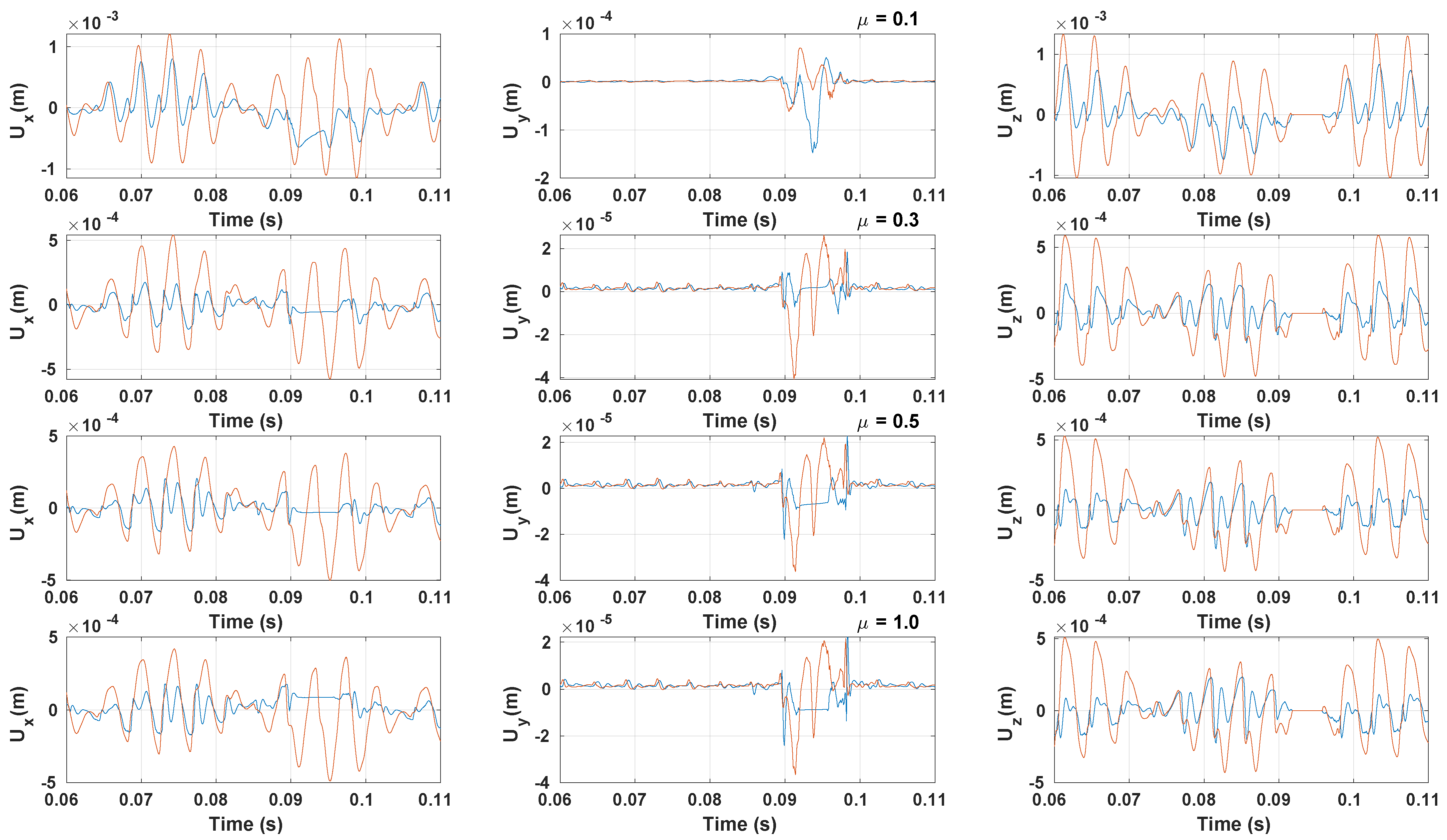
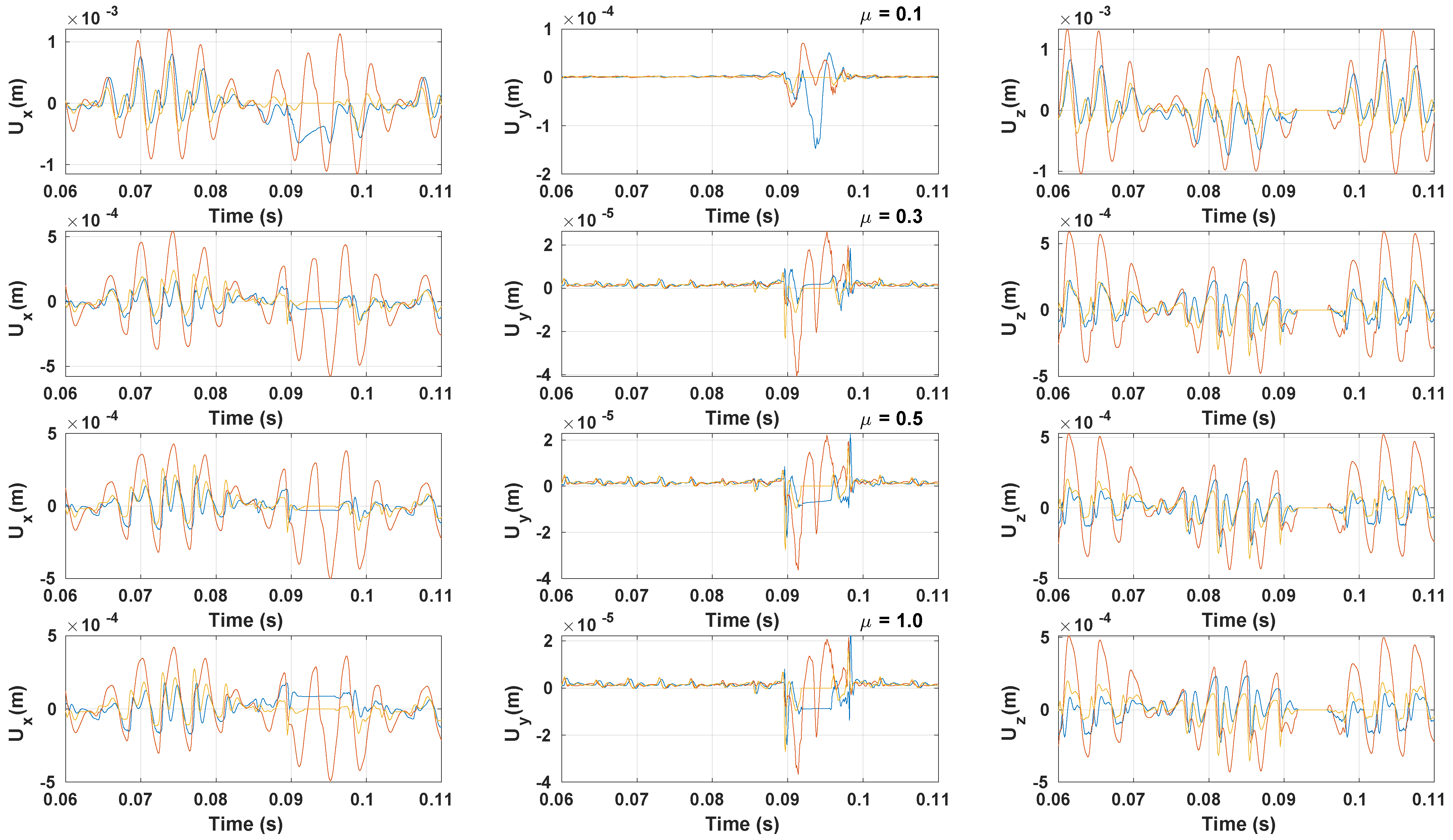
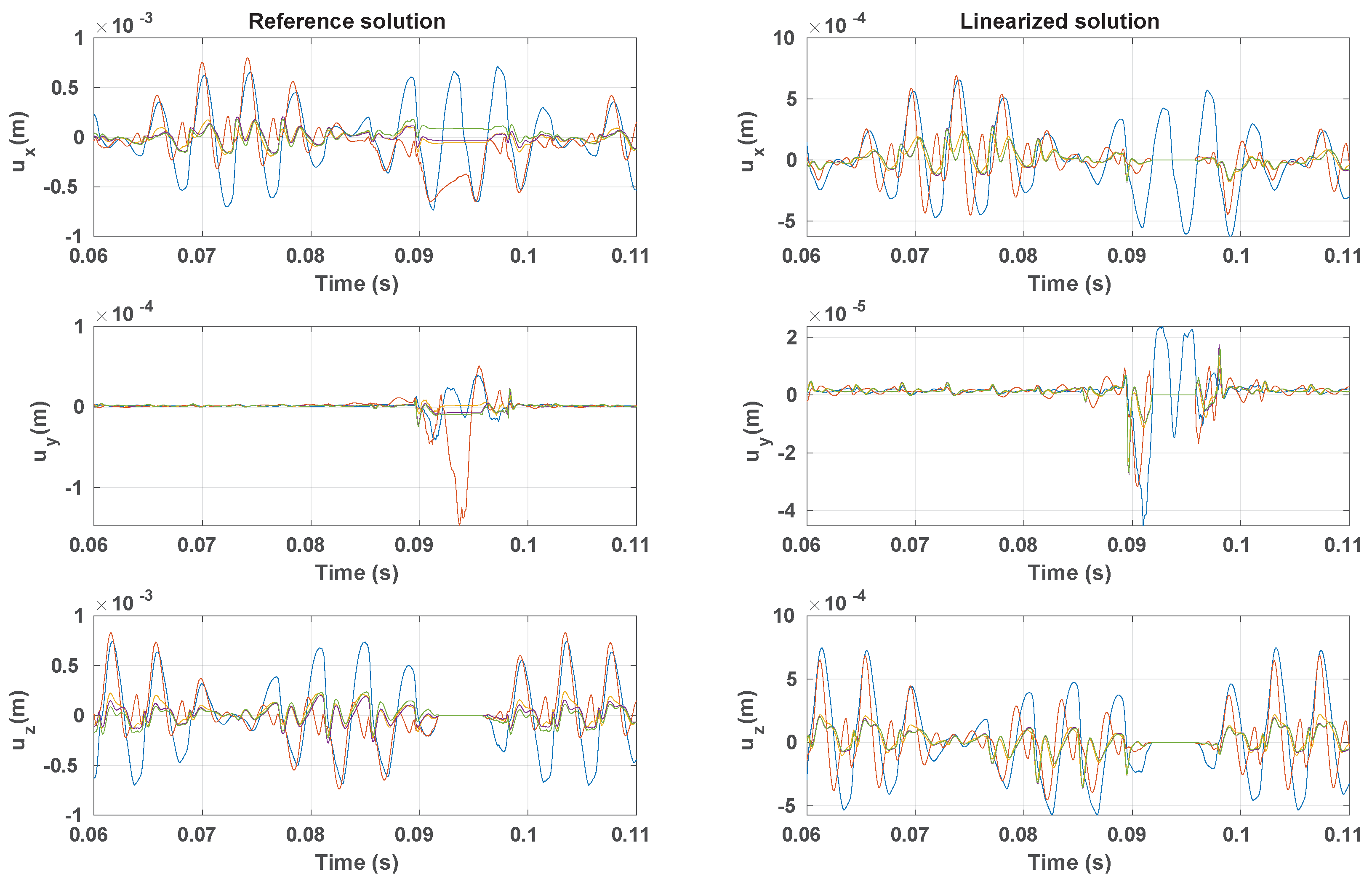
3.3.2. Coefficient of Friction Impact

The aim of this section is to study the coefficient of friction impact on the linearization process and on the vibrations response. A comparison between the displacement components of the linearized solution with the reference solution for various values of $\mu$ is displayed. A new boundary condition is proposed to improve the linearization method. Finally, the coefficient of friction impact on the vibrations amplitude is investigated.

Unlike the frictionless case, a greater difference between the vibrations is observed in Figure 17 for all values of $\mu$. The differences are especially observed in the contact active zone for the longitudinal and lateral vibrations displacement. Increasing the value of $\mu$ makes the vibrations constant in the contact patch for the reference solution. Indeed, the quasi-static rolling results show that increasing $\mu$ favors the stick regime. Hence, the longitudinal and lateral vibrations displacements remain constant in the contact patch. The constant value is not equal to 0 since the inertia changes the contact stiffness [22]. The boundary condition (31) used to treat the contact constraint is no longer valid for friction. A simple change of this condition is to impose an homogeneous displacement in the contact active zone as follows

$$\mathbf{w}=\mathbf{0}\mathrm{on}{\Gamma }_c^t$$

(39)

The results of the boundary conditions change are given in Figure 18 that illustrates the time evolution of the vibrations field for various values of $\mu$. A clear improvement of the linearized solution with respect to the reference solution is observed whether inside or outside the contact patch and especially for high values of $\mu$. The biggest difference is observed for $\mu =0.1$. Indeed, for this value of $\mu$, the nodes in the contact patch operate in the slip regime, which is clearly incompatible with the new boundary condition but still better than the previous one especially outside the contact zone. A more precise boundary condition to treat the frictional contact should depend on the contact regime. Now, we compare between the vibrations for different values of $\mu$ for both solutions.

Figure 19 shows the vibrations sensitivity with respect to the coefficient of friction. Both solutions give more or less the same observations expect for $\mu =0.1$ due to the incompatibility between the contact boundary condition and the friction slip regime. Larger vibrations are observed for the frictionless case for both solutions. Increasing $\mu$ results in damping the vibrations amplitude until reaching an invariant vibration response for $\mu >0.3$. This translates the saturation effect observed for the quasi-static rolling. The same saturation phenomenon is observed in [27] for advancing pin-loaded contacts with friction where the equations of motion are solved using the Green’s functions.

4. Conclusions

In this paper, an adapted two-step approach to simulate the nonlinear vibrations of a hyperelastic solid undergoing large deformations in contact with rigid plane is presented. The methodology allows not only the separation between the dynamics operating at different scales but also shows numerical robustness and consistency. The Coulomb friction law is used in the contact interface. This numerical approach is applied to a finite element model corresponding to a grooved cylinder. The linearization process seems to work very well for frictionless contact; however, significant differences can be observed for the case with frictional contact, especially for higher values of $\mu$. The change of the boundary condition in the contact active zone seems to improve the linearized solution. A much more precise condition in the contact active zone would probably depend on the friction (slip or stick) regime.

As previously mentioned, the example proposed and discussed in this paper corresponds to a grooved cylinder undergoing large deformation in contact with rigid plane. One of the most crucial next steps is to be able to provide an illustration of the feasibility of the proposed approach on a tire structure. Numerous future research can be carried out to increase the understanding of non-linear phenomena on tire structures. Although it is not possible to give an exhaustive list of topics of interest, some studies that seem to have a certain priority and interest may be considered:

• First of all, it can be noted that damping has been neglected in modeling; however, experiments show that vibration energy is not transported to the opposite of contact patch due to strong damping of tire structure for such relatively high frequencies. The vibration energy is thus concentrated close to the entrance and the exit of contact patch. Moreover the vibrations evolution in the circumferential direction shows the opposite observation; therefore, the addition of a suitable damping model seems important and is one of the priority issues to be explored. The inclusion of the Kelvin–Voigt model, often used to treat the viscosity of tire rubber, seems to be an interesting option [28].
• In a similar way, the modeling of friction at the contact interface should be completed by the consideration of the coefficient of rolling friction [29] in order to reproduce more realistic physical phenomena involved in tire/pavement interaction vibration and noise. Indeed, the consideration of only the coefficient of sliding friction force as proposed in this study may be not sufficient to accurately reproduce real phenomena of tire vibration response.
• It should be interesting to apply the proposed two-step approach on a real industrial tire structure and to compare the results with full experimental tests. One of the most important challenges may be to identify the different sources of nonlinear vibrations in order to identify and quantify the first-order physical phenomena involved. In this context, more realistic modeling including both tire rubber viscosity and Hertzian contact for polymorph materials or the model of contact 3D multi-layered structures with orthotropic material should be developed to reproduce more specifically the design of a real wheel tire.
• Extension of the prediction of non-linear vibrations in a real environment and in real conditions would also be interesting with the consideration of a more realistic pavement with imperfections. The road roughness excitation mechanism could be added to the proposed methodology by integrating the road texture in the normal gap function calculation. In this context, one of the main challenges for engineers working on the developments of optimization procedures for tire structures in a real environment should be the inclusions of modeling errors and uncertainties.
• The developments and combination of optimization procedures, genetic algorithms or artificial neural in relation with the proposed methodology should also be of prior interest to conduct parametric studies leading to increase the reliability and safety of tire structures subjected to complex and various external excitations.

References

- Sandberg, U.; Ejsmont, J.A. Tyre/Road Noise Reference Book; Informex: Kisa, Sweden, 2002. [Google Scholar]
- Li, T. Influencing parameters on tire–pavement interaction noise: Review, experiments and design considerations. Designs 2018, 2, 38. [Google Scholar] [CrossRef] [Green Version]
- Li, T.; Burdisso, R.; Sandu, C. Literature review of models on tire-pavement interaction noise. J. Sound Vib. 2018, 2, 357–445. [Google Scholar] [CrossRef]
- Ling, S.; Yu, F.; Sun, D.; Sun, G.; Xu, L. A comprehensive review of tire-pavement noise: Generation mechanism, measurement methods, and quiet asphalt pavement. J. Clean. Prod. 2021, 287, 125056. [Google Scholar] [CrossRef]
- Nackenhorst, U. The ALE-formulation of bodies in rolling contact: Theoretical foundations and finite element approach. Comput. Methods Appl. Mech. Eng. 2004, 193, 4299–4322. [Google Scholar] [CrossRef]
- Brinkmeier, M.; Nackenhorst, U.; Volk, H. A Finite Element Approach to the Transient Dynamics of Rolling Tires with Emphasis on Rolling Noise Simulation. Tire Sci. Technol. 2007, 35, 165–182. [Google Scholar] [CrossRef]
- De Gregoriis, D.; Naets, F.; Kindt, P.; Desmet, W. Development and validation of a fully predictive high-fidelity simulation approach for predicting coarse road dynamic tire/road rolling contact forces. J. Sound Vib. 2019, 452, 147–168. [Google Scholar] [CrossRef]
- Gonzalez Diaz, C.; Kindt, P.; Middelberg, J.; Vercammen, S.; Thiry, C.; Close, R.; Leyssens, J. Dynamic behaviour of a rolling tyre: Experimental and numerical analyses. J. Sound Vib. 2016, 364, 147–164. [Google Scholar] [CrossRef]
- Pinay, J.; Saito, Y.; Mignot, C.; Gauterin, F. Understanding the contribution of groove resonance to tire-road noise on different surfaces under various operating conditions. Acta Acust. 2020, 4, 1–12. [Google Scholar] [CrossRef]
- Ejsmont, J.A.; Sandberg, U.; Taryma, S. Influence of tread pattern on tire/road noise. SAE Transactions 1984, 93, 632–640. [Google Scholar] [CrossRef]
- Li, T. Influence of tread pattern on tire/road noise. Automot. Tire Noise Vib. 2020, 27–41. [Google Scholar] [CrossRef]
- Hauret, P. Méthodes Numériques Pour la Dynamique des Structures non Linéaires Incompressibles à Deux Échelles. Ph.D Thesis, Ecole Polytechnique, Palaiseau, France, 2004. [Google Scholar]
- Gonzalez, O. Exact energy and momentum conserving algorithms for general models in nonlinear elasticity. Comput. Methods Appl. Mech. Eng. 2000, 190, 1763–1783. [Google Scholar] [CrossRef] [Green Version]
- Biot, M.A. Mechanics of Incremental Deformations; John Wiley & Sons, Inc.: New York, NY, USA; London, UK; Sydney, Australia, 1965. [Google Scholar] [CrossRef] [Green Version]
- Valyaev, V. On approaches to simulation of rolling tire vibrations. Michelin Intern. Rep. 2016. [Google Scholar]
- Ogden, R.W. Non-Linear Elastic Deformations; Dover Publications Inc.: Mineola, NY, USA, 1997. [Google Scholar]
- Signorini, A. Questioni di elasticita non linearizzata e semilinearizzata. Rend. Mat. Delle Sue Appl. 1959, 18, 95–139. [Google Scholar]
- Yastrebov, V. Computational Contact Mechanics: Geometry, Detection and Numerical Techniques. Ph.D Thesis, École Nationale Supérieure des Mines de Paris, Paris, France, 2011. [Google Scholar]
- Wriggers, P. Constitutive Equations for Contact Interfaces. In Computational Contact Mechanics; Springer: Berlin/Heidelberg, Germany, 2006; pp. 69–108. [Google Scholar] [CrossRef]
- Simo, J.C.; Laursen, T.A. An augmented lagrangian treatment of contact problems involving friction. Comput. Struct. 1992, 42, 97–116. [Google Scholar] [CrossRef]
- Fortin, A.; Garon, A. Les Éléments Finis: De la Théorie à la Pratique. GIREF. 2020. Available online: https://giref.ulaval.ca/afortin/elements_finis.pdf (accessed on 14 December 2021).
- Winroth, J.; Andersson, P.; Kropp, W. Importance of tread inertia and damping on the tyre/road contact stiffness. J. Sound Vib. 2014, 333, 5378–5385. [Google Scholar] [CrossRef] [Green Version]
- Jazar, R.N. Tire Dynamics. Veh. Dyn. 2014, 95–163. [Google Scholar] [CrossRef]
- Chipato, E.T.; Shaw, A.D.; Friswell, M.I. Nonlinear rotordynamics of a MDOF rotor-stator contact system subjected to frictional and gravitational effects. Mech. Syst. Signal Process. 2021, 159, 107776. [Google Scholar] [CrossRef]
- Zhou, P.; Du, M.; Chen, S.; He, Q.; Peng, Z.; Zhang, W. Study on intra-wave frequency modulation phenomenon in detection of rub-impact fault. Mech. Syst. Signal Process. 2019, 122, 342–363. [Google Scholar] [CrossRef]
- Mlika, R.; Renard, Y.; Chouly, F. An unbiased Nitsche’s formulation of large deformation frictional contact and self-contact. Comput. Methods Appl. Mech. Eng. 2017, 325, 265–288. [Google Scholar] [CrossRef] [Green Version]
- Sundaram, N.; Farris, T. Mechanics of advancing pin-loaded contacts with friction. J. Mech. Phys. Solids 2010, 58, 1819–1833. [Google Scholar] [CrossRef]
- Scaraggi, M.; Persson, B. Friction and universal contact area law for randomly rough viscoelastic contacts. J. Phys. Condens. Matter 2015, 27, 105102. [Google Scholar] [CrossRef] [PubMed]
- Alaci, S.; Muscă, I.; Pentiuc, Ș.G. Study of the Rolling Friction Coefficient between Dissimilar Materials through the Motion of a Conical Pendulum. Materials 2020, 13, 5032. [Google Scholar] [CrossRef] [PubMed]