Uncertainty Analysis Based on Kriging Meta-Model for Acoustic-Structural Problems

Abstract

This paper consists of evaluating the performance of a vibro-acoustic model in the presence of uncertainties in the geometric and material parameters of the model using Monte Carlo simulations (MCS). The purpose of using a meta-model is to reduce the computational cost of finite element simulations. Uncertainty analysis requires a large sample of MCS to predict the effect of uncertain parameters on the system response. So, if this study is done through the finite element method (FEM), then the computational cost will be very important. Furthermore, for that, we use meta-models to be able to conduct an efficient uncertainty analysis more quickly. In the present contribution, the approximated meta-model is verified and validated using error measures and cross-validation (CV). Then, the uncertainty analysis is performed by Monte Carlo simulations using the computed Kriging meta-model. The developed methodology has been applied in two vibro-acoustic models. In these two models, the covariance of uncertainty of geometric and physical (elasticity and density) parameters are equal to 2% and 5% respectively. The obtained results prove that the suggested methodology of uncertainty propagation based on the Kriging meta-model can be considered as a very efficient and sufficiently accurate approach for the quantification of uncertainties in acoustic-structural systems.

1. Introduction

The problem of interaction between flexible vibrating structures and an enclosed cavity is a complex domain that has been of great attentions for researchers in different fields such as automobile compartments, airplane cabins, etc. The vibration energy generated from various sources is transmitted into the compartment cavity through structural connections. Thus, vibration characteristics of the cavity and its boundary are very important factors which dominate acoustic response in a vehicle passenger compartment. The knowledge of acoustic resonances and their own modes (i.e., sound pressure distributions) is an essential task in the study of the interaction between the vibrating surface and the enclosed cavity, and ultimately in determining the level of the resulting interior noise. Craggs [1] presented a verification of finite element predictions of acoustic resonances in a vehicle cabin, while in [2], Nefsk et al. presented an experimental verification of the finite element method to predict the noise reduction in the automobile. In [3], the author presented an active vibration control system for structural acoustic coupling of a 3D vehicle cabin model. The structural-acoustic coupling system is analyzed by combining the structural data from modal testing with the acoustic data from the finite element method. An excellent review was given by [4,5] to investigate the vibro-acoustic behavior of such systems, such as modal interaction of coupled structural-acoustic systems. Redonnet and Cunha [6] suggested an extended approach to numerically simulate complex noise problems. Several authors investigated in their studies the phenomenon of fluid–structure interaction applied to different applications [7,8,9], to determine the resonances of an irregularly shaped cavity. The finite element method (FEM) denotes a very powerful method, which can be used in order to obtain an approximate solution to the response of the coupled system. Dammak et al. [10] studied the vibro-acoustic response of a vehicle cabin in presence of uncertainties.

In general, it is well known that the numerical study of the frequency response of the vibro-acoustic field without considering the uncertainty associated with different parameters has achieved great attention. However, there are many sources of uncertainty such as errors related to manufacturing, material characteristics, boundary conditions, (etc.), that needed to be integrated in the study to ensure the robustness and reliability of results. Taking into account of uncertainties in systems analysis is a difficult domain including the following steps: quantification and identification of uncertainty, uncertainty propagation and post-processing to measure the influence of these uncertainties on the behaviour of the system. The main approaches for the inclusion of these uncertainties are probabilistic methods [11,12] which the uncertain parameters can be modeled as random variables through the description of their probability density functions. Recently, the probabilistic modeling of vibro-acoustic problems has received the attention of some researchers [13,14]. Among the probabilistic methods, the frequently used one is the statistical approach or sampling technique, like the Monte Carlo simulations (MCS) [15,16]. This technique requires a large number of samples of the input variables to have reasonable accuracy. The problem is then solved for each realization. This method is widely used because it is simple to implement and very robust. However, the number of realisation should be large enough, i.e., ${10}^5$ or ${10}^6$ deterministic FEM need to be executed in order to obtain accurate results. In [17], the author used only MCS to account for uncertainties in vibro-acoustic problem which took a huge computational cost in its development process. Several authors used the non-parametric probabilistic approach to model the effect of uncertainties in their vibro-acoustic studies of car models [18,19,20]. The spectral stochastic method is also an alternative solution for stochastic problems. The basic concept of this method is to use a series expansion to model the relationship between the uncertainty of the input and output variability. The generalized polynomial chaos (gPC), one of the spectral stochastic methods, has already been applied in the modeling of uncertainty in various areas, such as structural dynamics [21], fluid dynamics [22] and acoustics [23,24].

Generally when using computationally expensive simulation codes in complex engineering problems, it becomes impractical to perform a large number of simulations for the purpose of uncertainty quantification or design optimization. A better alternative lies in the use of approximations of the original models, which are often called meta-models. A surrogate model can be understood as a “model of model”. It is a statistical model of the response surface of a simulation model. A surrogate model describes the relationship between inputs (i.e., model’s adjustable parameters) and outputs (i.e., the performance measure of the simulation model) [25]. Surrogate models have primarily been developed for approximating deterministic simulations. Recent developments have explored their use in probabilistic analysis [26,27,28] and design optimization [29,30,31]. In [32], the authors performed a comprehensive study regarding the application of meta-models in mechanical systems. Response surface methodology (RSM) [33,34,35], Kriging [36,37,38] and neural networks [39,40] are the most commonly used meta-models.

This work presents the harmonic analysis of vibro-acoustic systems with taking into account uncertainties in geometrical and material parameters. The Kriging method is investigated to approximate the original model by representing the relationship between input parameters and output responses. In the proposed probabilistic method based on surrogate model, deterministic FEM are carried out to obtain the physical response of the system. MCS is performed by using Kriging meta-model in order to study the performance of the vibro-acoustic problems.

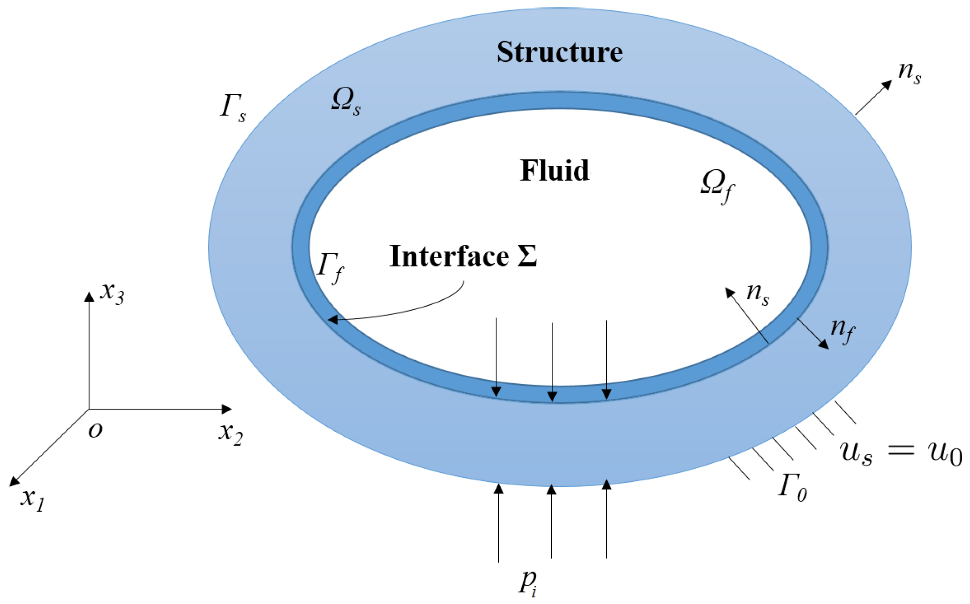
2. Vibro-Acoustic Formulation

In the presence of a harmonic variation and a closed cavity, ${\Omega }_f$, the acoustic pressure $p_i$ can be calculated using the Helmholtz equation as [41,42]:

$$\Delta p_i+k^2{p}_i=0\mathrm{in}{\Omega }_f$$

(1)

where $\Delta$ represents the Laplacian operator, the wave number is calculated by $k=\frac{\omega }{c}$ and c denotes the sound speed in the environment. The boundary conditions of the vibro-acoustic system is presented in Figure 1.

$$\frac{\partial p_i}{\partial n}={\rho }_f{\omega }^2{u}_s\mathrm{on}\Sigma$$

(2)

where $u_s$ is the structural displacement, ${\rho }_f$ denotes the density of the fluid. In the presence of a rigid surface, $\frac{\partial p_i}{\partial n}=0$. It is assumed that the structure is elastic and then its response can be determined from the local equations [43]:

$$\mathrm{div}\sigma \left(u_s\right)+{\rho }_s{\omega }^2{u}_s=0\mathrm{in}{\Omega }_s$$

(3)

where the density of the structure is denoted by ${\rho }_s$ and $\sigma \left(u_s\right)$ presents the stress tensor.

$$\sigma \left(u_s\right)·n=p_i\mathrm{on}{\Gamma }_s$$

(4)

$$u_s=u_0\mathrm{on}{\Gamma }_0$$

(5)

where ${\Gamma }_s\cap {\Gamma }_0=\left\{0\right\}$ and ${\Gamma }_s\cup {\Gamma }_0=\Sigma$. In most practical cases, the finite element method is used in order to solved numerically Equation (1). It is a coupled problem between the internal acoustic pressure and the vibration of the structure. The finite element discretization of the structural part and that of the fluid leads to the equations of motion corresponding to each part as follow [10,43,44]:

$$\left[{\mathit{M}}_{\mathit{s}}\right]\left\{{\ddot{\mathit{U}}}_{\mathit{s}}\right\}+\left[{\mathit{B}}_{\mathit{s}}\right]\left\{{\dot{\mathit{U}}}_{\mathit{s}}\right\}+\left[{\mathit{K}}_{\mathit{s}}\right]\left\{{\mathit{U}}_{\mathit{s}}\right\}=\left\{{\mathit{F}}_{\mathit{s}}\right\}+\left\{{\mathit{F}}_{\mathit{sf}}\right\}$$

(6)

$$\left[{\mathit{M}}_{\mathit{f}}\right]\left\{\ddot{\mathit{P}}\right\}+\left[{\mathit{B}}_{\mathit{f}}\right]\left\{\dot{\mathit{P}}\right\}+\left[{\mathit{K}}_{\mathit{f}}\right]\left\{\mathit{P}\right\}=\left\{{\mathit{F}}_{\mathit{f}}\right\}+\left\{{\mathit{F}}_{\mathit{fs}}\right\}$$

(7)

where $\left[{\mathit{M}}_{\mathit{s}}\right]$ is the mass matrix of the structure part, $\left[{\mathit{K}}_{\mathit{s}}\right]$ is the equivalent rigidity matrix of the structure, $\left\{{\mathit{F}}_{\mathit{s}}\right\}$ denotes the vector of external forces applied to the structure and $\left\{{\mathit{U}}_{\mathit{s}}\right\}$ represents the vector of nodal displacements. $\left[{\mathit{M}}_{\mathit{f}}\right]$ denotes the mass matrix of the fluid, $\left[{\mathit{K}}_{\mathit{f}}\right]$ represents the equivalent stiffness matrix of the fluid, $\left\{{\mathit{F}}_{\mathit{f}}\right\}$ is the vector of the external forces applied to the fluid, and $\left\{\mathit{P}\right\}$ denotes the vector of acoustic nodal pressures. $\left\{{\mathit{F}}_{\mathit{sf}}\right\}=-\left[\mathit{A}\right]\left\{\mathit{P}\right\}$ represents the vector of forces from the fluid portion acting on the structural part while $\left[\mathit{A}\right]$ represents the matrix of the coupled system at the boundary surfaces.

$\left\{{\mathit{F}}_{\mathit{fs}}\right\}={\left[\mathit{A}\right]}^{\mathrm{T}}\left\{{\ddot{\mathit{U}}}_{\mathit{s}}\right\}$ denotes the vector of structural forces acting on the fluid portion.

The motion equation for the coupled fluid–structure system can be written in a matrix form as follows:

$$\left[\begin{array}{cc}{\mathit{M}}_{\mathit{s}}& 0\\ -{\mathit{A}}^{\mathrm{T}}& {\mathit{M}}_{\mathit{f}}\end{array}\right]·\left(\begin{array}{c}{\ddot{\mathit{U}}}_{\mathit{s}}\\ \ddot{\mathit{P}}\end{array}\right)+\left[\begin{array}{cc}{\mathit{B}}_{\mathit{s}}& 0\\ 0& {\mathit{B}}_{\mathit{f}}\end{array}\right]·\left(\begin{array}{c}{\dot{\mathit{U}}}_{\mathit{s}}\\ \dot{\mathit{P}}\end{array}\right)+\left[\begin{array}{cc}{\mathit{K}}_{\mathit{s}}& \mathit{A}\\ 0& {\mathit{K}}_{\mathit{f}}\end{array}\right]·\left(\begin{array}{c}{\mathit{U}}_{\mathit{s}}\\ \mathit{P}\end{array}\right)=\left(\begin{array}{c}{\mathit{F}}_{\mathit{s}}\\ {\mathit{F}}_{\mathit{f}}\end{array}\right)$$

(8)

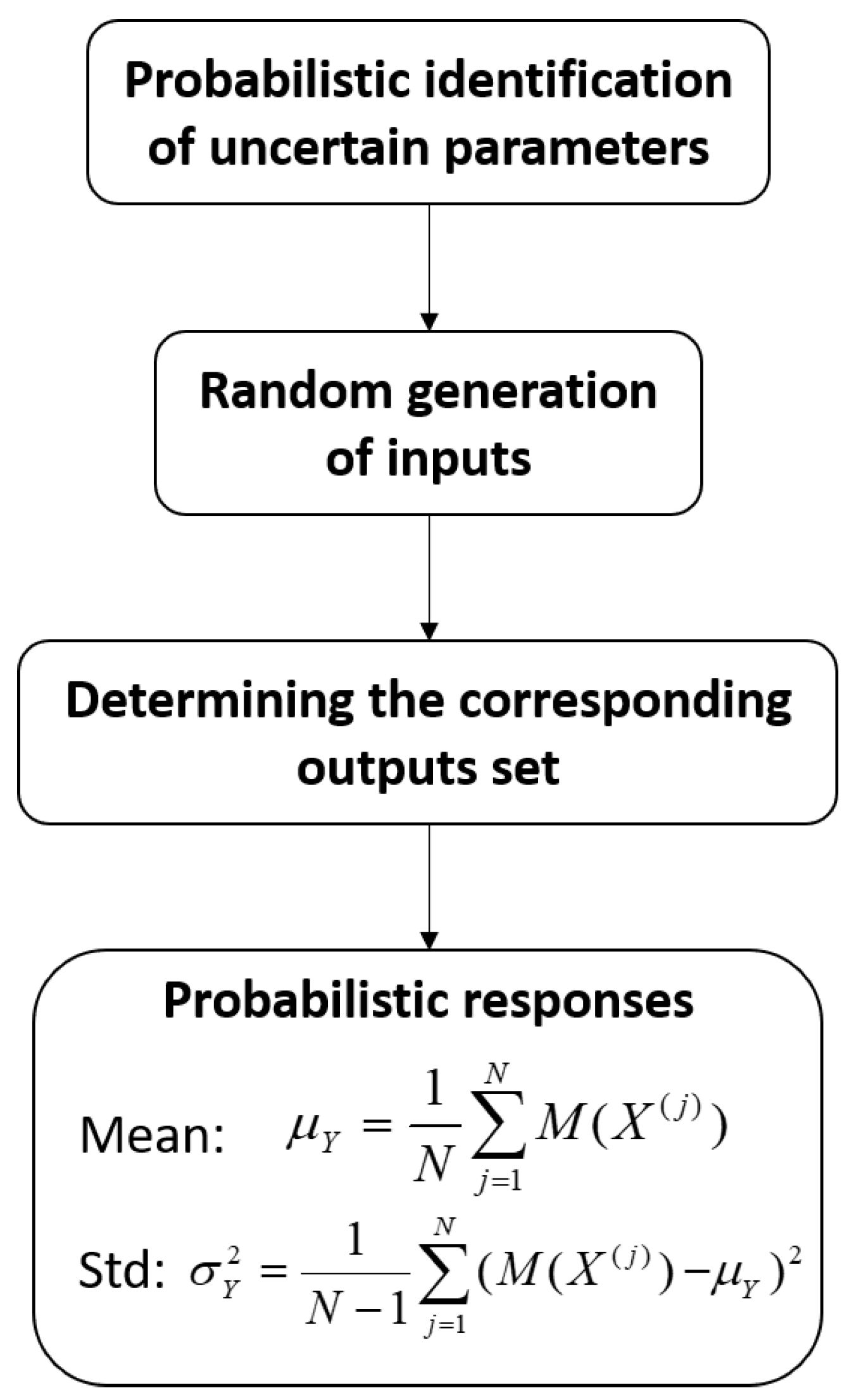
3. Monte Carlo Simulations

The MCS method provides successive resolutions of a deterministic system incorporating uncertain parameters described by random variables. It generates random samples for all uncertain parameters. For each iteration, a set of parameters is obtained and a deterministic calculation, according to well-defined numerical models (FEM) or analytical, is performed. The main advantage of this technique is its applicability to any system, regardless of its complexity (linear, non-linear, etc.) and size. A reasonable precision of the results requires a large number of points. This makes this method prohibitive in terms of calculation cost. The standard MCS approach considers functions of the following form:

$$\mathit{Y}=\chi \left(\mathit{X}\right)$$

(9)

where $\chi$ denotes the model, $\mathit{X}={[X_1,X_2,\dots ,X_n]}^{\mathrm{T}}$ represents the vector of uncertain input parameters and $\mathit{Y}$ is the vector of estimated outputs. The algorithm of this method can be summarized in the flowchart presented in Figure 2:

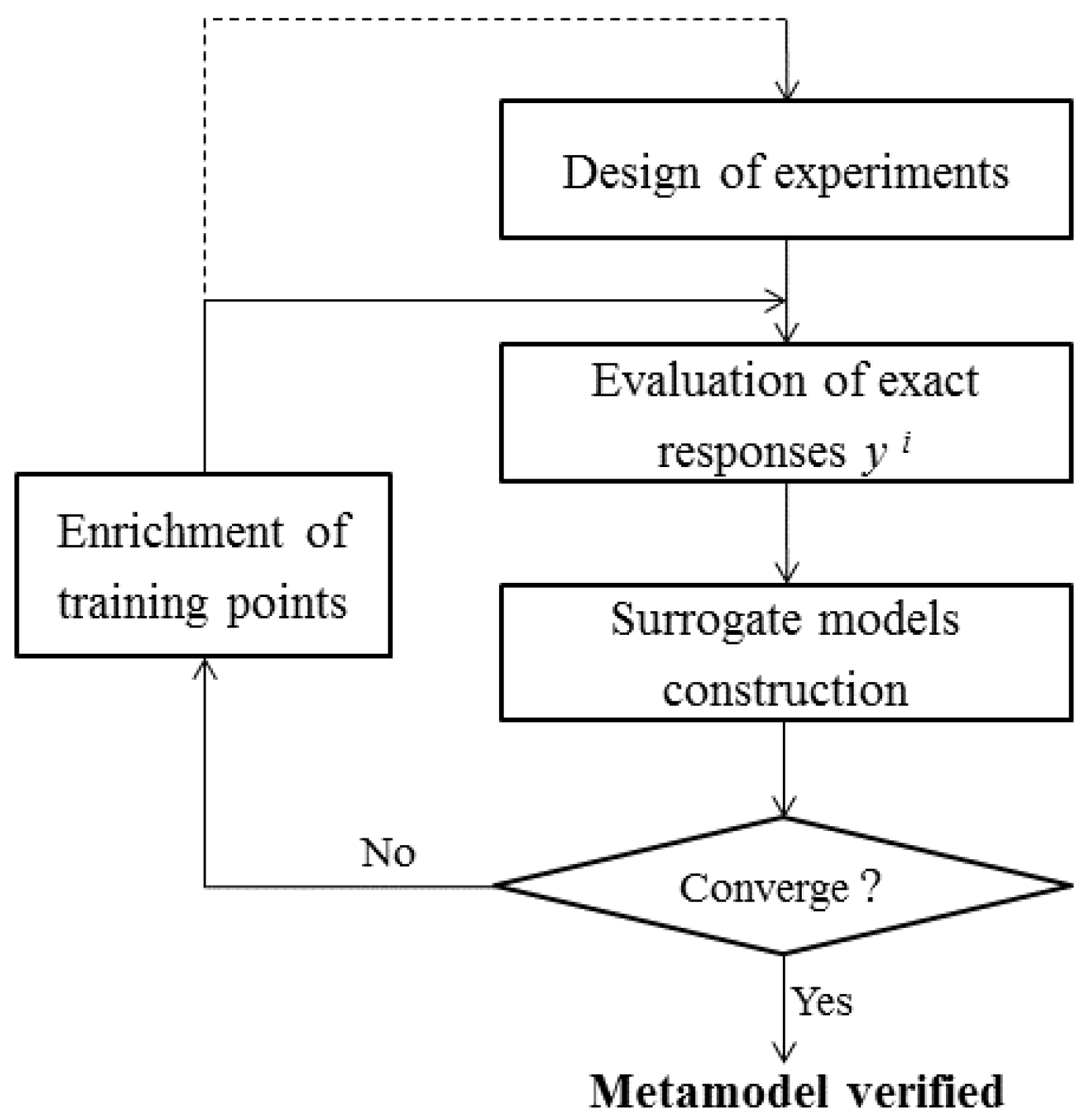
4. Surrogate Modeling Techniques

4.1. Generality

Nowadays, meta-model approaches are widely used in different engineering field. These models are used to construct approximations of the finite element method and describe the relationship between the input parameters and the responses of the system. Thus, the calculation cost is reduced. In this study, the meta-models are used to estimate the sound pressure level of coupled acoustic-structural problems.

To start, let us consider a m-dimensional problem. We use $\mathit{x}={\{x_1,x_2,\dots ,x_m\}}^{\mathrm{T}}$ to denote the design variables with m dimensions, ${\mathit{x}}_S={\{{\mathit{x}}^{\left(1\right)},{\mathit{x}}^{\left(2\right)},\dots ,{\mathit{x}}^{\left(n\right)}\}}^{\mathrm{T}}$ to indicate a set of samples with n design points, and ${\mathit{y}}_S={\{f\left({\mathit{x}}^{\left(1\right)}\right),\dots ,f\left({\mathit{x}}^{\left(n\right)}\right)\}}^{\mathrm{T}}$ to signify the corresponding outputs responses of the sample set. The pair $({\mathit{x}}_S,{\mathit{y}}_S)$ indicates the sampled data set. The objective of the meta-modeling is to build a meta model that predict the output of any untried point $\mathit{x}$, thus, to estimate $y\left(\mathit{x}\right)$ based on the pair $({\mathit{x}}_S,{\mathit{y}}_S)$. The implementation of a surrogate model is a multi-step process. As presented by Forrester et al. [25], in order to build a good approximation of the original model, we need several steps: Sampling plans, exact evaluations, constructing a surrogate and verifying meta-model quality. The flowchart of this process is presented in Figure 3.

The surrogate modelling approach first applies design of experiments (DOEs). Classical DOEs (fractional factorial designs, central composite designs, etc.) tend to spread the sample points around the border and only put a few points in the interior of the design space. They are primarily used for screening purposes and to build polynomial meta-models. For this, the Latin hypercube sampling (LHS), proposed by McKay et al. [45], is selected to repeat sampling in the design space and then chooses a type of meta-model to represent the sampled data. Thus, the original analysis code can be replaced by the surrogate model during the uncertainty process.

4.2. Kriging Meta-Model

Generally, the Kriging method is very applied today because of its robustness and the quality of the approximation it can provide. In addition, it provides an estimate of the least squares error of the process that it estimates. The modern framework of Kriging (also called Gaussian process modeling) is based on the fact that the substitution function is assumed to be an achievement of a Gaussian process denoted $y\left(\mathit{x}\right)$. Thus, the response $y\left(\mathit{x}\right)$ can be expressed as follows:

$$y\left(\mathit{x}\right)=G\left(\mathit{x}\right)+Z\left(\mathit{x}\right)$$

(10)

where $G\left(\mathit{x}\right)$ is usually given as a linear combination of basic polynomial functions:

$$G\left(\mathit{x}\right)=\sum _{i=1}^{p-1}{\beta }_i{f}_i\left(\mathit{x}\right)$$

(11)

where $\mathit{f}\left(\mathit{x}\right)={[f_0\left(\mathit{x}\right),f_1\left(\mathit{x}\right),\dots ,f_{p-1}\left(\mathit{x}\right)]}^{\mathrm{T}}$ represents the vector of regression basis function and the column vector $\beta ={[{\beta }_0,{\beta }_1,\dots ,{\beta }_{p-1}]}^{\mathrm{T}}$ is the vector of regression coefficients and $Z\left(\mathit{x}\right)$ is a stochastic process (random function) with zero mean $\left(\mathbb{E}\right[Z\left(\mathit{x}\right)]=0)$, a variance ${\sigma }^2$ and non-zero covariance given by:

$$Cov(Z\left(\mathit{x}\right)-Z\left({\mathit{x}}^{\prime }\right))={\sigma }^{2}R(\mathit{x},{\mathit{x}}^{\prime })$$

(12)

where $R(\mathit{x},{\mathit{x}}^{\prime })$ denotes the correlation function between the estimated sampling points $\mathit{x}$ and ${\mathit{x}}^{\prime }$ in the design space. It controls the smoothness of the resulting model. The correlation function in Equation (12) affects the smoothness of the model. A product of correlation functions is generally used to construct n dimensional ones:

$$R(\mathit{x},{\mathit{x}}^{\prime })=\prod _{i=1}^{m}R(x_i,x_i^{\prime })$$

(13)

where m is the dimension of design variables and $x_i$ and $x_i^{\prime }$, respectively, are the ith component of the sampling design point $\mathit{x}$ and ${\mathit{x}}^{\prime }$, respectively.

According to [46] two commonly applied functions are the exponential (Equation (14)) and the Gaussian correlation functions (Equation (15)):

$$R(\mathit{x},{\mathit{x}}^{\prime })=exp\left[-\sum _{i=1}^m{\theta }_i|x_i-x_i^{\prime }|\right]$$

(14)

$$R(\mathit{x},{\mathit{x}}^{\prime })=exp\left[-\sum _{i=1}^m{\theta }_i{|x_i-x_i^{\prime }|}^2\right]$$

(15)

with $\mathit{\theta }={[{\theta }_1,\dots ,{\theta }_m]}^{\mathrm{T}}$ denotes the vector of unknown parameters of the correlation function. The Kriging estimator at a given point $\mathit{x}$ is by definition a Gaussian random variable obtained as a linear combination of the observations and which is called the best linear unbiased estimator (BLUE) [47]:

$$\widehat{y}\left(\mathit{x}\right)={\mathit{f}}^{\mathrm{T}}\left(\mathit{x}\right)\mathit{\beta }+{\mathit{r}}^{\mathrm{T}}\left(\mathit{x}\right){\mathit{R}}^{-1}({\mathit{y}}_S-{\mathit{F}}^{\mathrm{T}}\mathit{\beta })$$

(16)

where ${\mathit{f}}^{\mathrm{T}}\left(\mathit{x}\right)$ is the regression basis function vector of the untired site $\mathit{x}$, $\mathit{\beta }$ denotes the vector of estimated regression coefficients, $\mathit{r}\left(\mathit{x}\right)={[R(\mathit{x},{\mathit{x}}^{\left(1\right)}),R(\mathit{x},{\mathit{x}}^{\left(2\right)}),\dots ,R(\mathit{x},{\mathit{x}}^{\left(n\right)})]}^{\mathrm{T}}$ represents the vector of correlation functions between the untried sites $\mathit{x}$ and the m sample points, $\mathit{R}$ is the $m\times m$ matrix of correlation functions for the fitting sample, ${\mathit{y}}_S$ represents the vector of the observed responses in the fitting sample and the term $({\mathit{y}}_S-{\mathit{F}}^{\mathrm{T}}\mathit{\beta })$ represents the vector of residuals for all fitting points when the stochastic term of the model is neglected. $\mathit{F}$ represents the model matrix as follows:

$$\mathit{F}=\left[\begin{array}{cccccccccc}1& x_1^{\left(1\right)}& \dots & x_m^{\left(1\right)}& x_1^{\left(1\right)}{x}_2^{\left(1\right)}& \dots & x_{m-1}^{\left(1\right)}{x}_m^{\left(1\right)}& {(x_1^{\left(1\right)})}^2& \dots & {(x_m^{\left(1\right)})}^2\\ 1& x_1^{\left(2\right)}& \dots & x_m^{\left(2\right)}& x_1^{\left(2\right)}{x}_2^{\left(2\right)}& \dots & x_{m-1}^{\left(1\right)}{x}_m^{\left(2\right)}& {(x_1^{\left(2\right)})}^2& \dots & {(x_m^{\left(2\right)})}^2\\ ⋮& ⋮& \ddots & ⋮& ⋮& \ddots & ⋮& ⋮& \ddots & ⋮\\ 1& x_1^{\left(n\right)}& \dots & x_m^{\left(n\right)}& x_1^{\left(n\right)}{x}_2^{\left(n\right)}& \dots & x_{m-1}^{\left(1\right)}{x}_m^{\left(n\right)}& {(x_1^{\left(n\right)})}^2& \dots & {(x_m^{\left(n\right)})}^2\end{array}\right]$$

(17)

In order to be able to construct the Kriging surrogate model, we first need to determine the correlation parameters of the vector $\mathit{\theta }$ in Equation (14) or Equation (15), the regression coefficients of the vector $\mathit{\beta }$ in Equation (11) and the variance of the stochastic model ${\sigma }^2$ in (Equation (12)). The method, currently the most used to determine all these parameters, is based on the statistical framework of Kriging and in particular that of Gaussian processes. Indeed, it proposes to determine these parameters by maximizing the likelihood function.

$$L(\mathit{\beta },{\sigma }^2,\mathit{\theta })=\frac{1}{\sqrt[n]{2\pi {\sigma }^2}\sqrt{\left|\mathit{R}\right(\mathit{\theta }\left)\right|}}exp\left[-\frac{{({\mathit{y}}_S-{\mathit{F}}^{\mathrm{T}}\mathit{\beta })}^{\mathrm{T}}{\mathit{R}}^{-1}\left(\mathit{\theta }\right)({\mathit{y}}_S-{\mathit{F}}^{\mathrm{T}}\mathit{\beta })}{2{\sigma }^2}\right]$$

(18)

In practice, we apply the natural logarithm on the expression of the likelihood and we obtain:

$$ln\left(L\right)=-\frac{n}{2}ln\left(2\pi \right)-\frac{n}{2}ln\left({\sigma }^2\right)-\frac{1}{2}ln\left(\right|\mathit{R}\left(\mathit{\theta }\right)\left|\right)-\frac{{({\mathit{y}}_S-{\mathit{F}}^{\mathrm{T}}\mathit{\beta })}^{\mathrm{T}}{\mathit{R}}^{-1}\left(\mathit{\theta }\right)({\mathit{y}}_S-{\mathit{F}}^{\mathrm{T}}\mathit{\beta })}{2{\sigma }^2}$$

(19)

The likelihood is maximal when its derivatives with respect to $\mathit{\beta }$ and ${\sigma }^2$ are setting to zero, thus gives:

$$\widehat{\mathit{\beta }}={\left({\mathit{F}}^{\mathrm{T}}{\mathit{R}}^{-1}\mathit{F}\right)}^{-1}{\mathit{F}}^{\mathrm{T}}{\mathit{R}}^{-1}{\mathit{y}}_S,$$

(20)

and

$${\widehat{\sigma }}^2=\frac{{({\mathit{y}}_S-{\mathit{F}}^{\mathrm{T}}\mathit{\beta })}^{\mathrm{T}}{\mathit{R}}^{-1}\left(\mathit{\theta }\right)({\mathit{y}}_S-{\mathit{F}}^{\mathrm{T}}\mathit{\beta })}{n}$$

(21)

The optimal values of $\mathit{\theta }$ are determined by solving the nonlinear optimization problem of the maximization of the likelihood function:

$$\begin{array}{cccc}\hfill & \underset{\theta }{\max }\hfill & \hfill & L\left(\mathit{\theta }\right)=-\frac{1}{2}[n(ln\left(2\pi \right)+ln\left({\widehat{\sigma }}^2\right))+ln\left(\right|\mathit{R}\left|\right)]\hfill \\ \hfill & \mathrm{s}.\mathrm{t}.\hfill & \hfill & {\theta }_i>0,i=1,\dots ,m\hfill \end{array}$$

(22)

Thus, by solving this optimization problem, the estimators $\widehat{\mathit{\beta }}$ and ${\widehat{\sigma }}^2$ can be calculated and then the model $\widehat{y}\left(\mathit{x}\right)$ is completely defined by Equation (16).

4.3. Metamodel Validation

It is necessary to assess the quality of the surrogate model after its construction. The quality of a surrogate model can be determined by several methods such as error measures and cross validation [47].

4.3.1. Error Measures

This method consists of studying the residuals of the model, i.e., the difference between the response of the original model $y^{\left(i\right)}$ and the value predicted by the meta-model ${\widehat{y}}^{\left(i\right)}$. The smaller the error, the better the quality of the estimator. The most popular measures are maximum absolute error (MAE), relative mean error (RME) and root mean squared error (RMSE) which can be expressed as follow:

$$\begin{array}{ccc}\hfill \mathrm{MAE}=max\left|y^{\left(i\right)}-{\widehat{y}}^{\left(i\right)}\right|,& \hfill & \hfill i=1,2,\dots ,n_t\end{array}$$

(23)

$$\mathrm{RME}=\frac{1}{n_t}\sum _{i=1}^{n_t}\left|\frac{y^{\left(i\right)}-{\widehat{y}}^{\left(i\right)}}{y^{\left(i\right)}}\right|$$

(24)

$$\mathrm{RMSE}=\sqrt{\frac{1}{n_t}\sum _{i=1}^{n_t}{\left(y^{\left(i\right)}-{\widehat{y}}^{\left(i\right)}\right)}^2}$$

(25)

where $n_t$ is the number of test points needed to calculate the error measures. The lower these measurements, the more accurate the meta-model.

4.3.2. Cross Validation

Another way to assess the quality of a surrogate model is cross validation (CV) [48]. In CV, samples data are divided into training points to build the model, and test points to assess its quality. The mean squares error (MSE), for ‘leave-one-out CV’ is expressed as:

$${\mathrm{MSE}}_{\mathrm{CV}}=\frac{1}{n}\sum _{i=1}^n{\left(y^{\left(i\right)}-{\widehat{y}}_{-i}^{\left(i\right)}\right)}^2$$

(26)

where $y^{\left(i\right)}$ is the response at ${\mathit{x}}^{\left(i\right)}$ from sample data and ${\widehat{y}}_{-i}^{\left(i\right)}$ denotes the estimation at ${\mathit{x}}^{\left(i\right)}$ using the meta-model built from all sampling points except $({\mathit{x}}^{\left(i\right)},y^{\left(i\right)})$ [49].

5. Numerical Examples

In the proposed method, the deterministic FEM is used to get the response feature at the training points that are generated using Latin hypercube sampling (LHS), the meta-model is employed to illustrate the relationship between inputs (design points) and outputs (responses), and then uncertainty analysis is carried out by using MCS based on surrogate model. In this section, the feasibility of the proposed methodology for uncertainty analysis based on surrogate model is applied on two vibro-acoustic models.

5.1. Structural-Acoustic Model

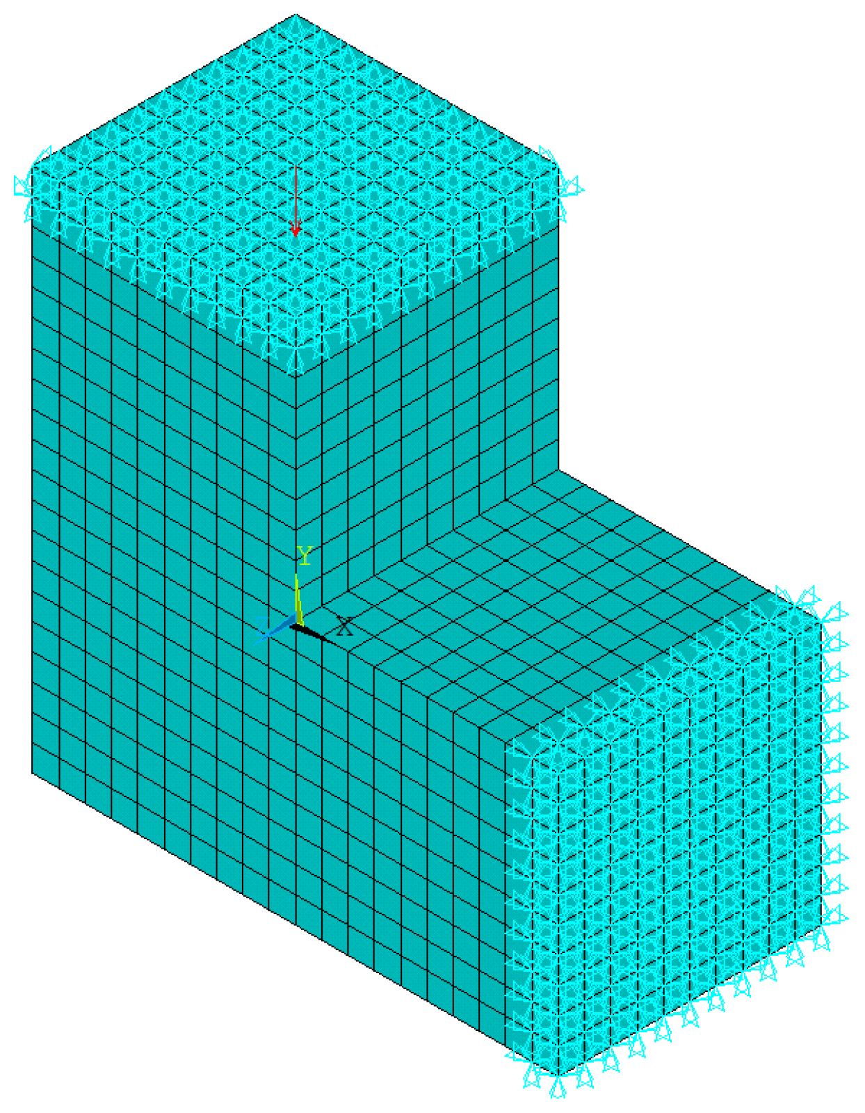
5.1.1. Deterministic FEM

The deterministic model consists of two aluminium flexible plates 1 and 2 with thickness $t_1=2$ mm and $t_2=4$ mm as shown in Figure 4 [50]. These plates are imposed on the right surface and on the top surface of the acoustic cavity, respectively. The remaining surfaces of the acoustic cavity are perfectly rigid and the system composed of flexible plates and acoustic cavity presents a coupled structural-acoustic problem. Numerical simulation of the vibro-acoustic response are performed using the commercial software ANSYS-APDL. Regarding the discretization of the internal fluid and the plates, 3000 and 200 elements are adopted, respectively, for the fluid and the structure. The internal fluid is modeled by Fluid30 elements having 8-nodes with one degree of freedom per node: the acoustic pressure. The flexible plates are modeled by Shell181 elements having 4-node with six degrees of freedom at each node: 3 translations in the x, y and z directions and 3 rotations about the x, y and z axes (see Figure 5). The adopted boundary conditions were fluid–structure interface at all free nodes of the aluminium plates. All the nodes at the plates border were constrained.

The finite element method (FEM) is used to study the sound pressure level (SPL) at point G2 as shown in Figure 6. This SPL can be determined using Equation (27) [10]:

$${\mathrm{SPL}}_{dB}=20{log}_{10}\left(\frac{P}{P_{ref}}\right)$$

(27)

with P is the acoustic pressure at G2 and $P_{ref}=20\mathsf{\mu }$Pa represents the acoustic pressure of human hearing.

5.1.2. Proposed Uncertainty Analysis Based on Surrogate Model

An accurate response surface is obtained from a minimum number of design points in the given sample space. The design sample space is constructed using Latin hypercube sampling (LHS) [45]. After the design of experiments process, several combinations of input parameters and their corresponding responses are obtained. The material parameters (elasticity and density) and the thicknesses of the aluminum plates are taken the uncertain variables in this study as shown in

Table 1. Characteristics of random variables.

Variables	Mean Value	Cov	Distribution Type
E (Pa)	2.1 × ${10}^{11}$	0.05	Normal
$\rho$ (kg/m${}^3$)	7850	0.05	Normal
$t_1$ (mm)	4	0.02	Uniform
$t_2$ (mm)	2	0.02	Uniform

.

For the assumed geometric constraints, design of experiment (DOE) points are generated. Mathematical model is then generated by performing a Kriging prediction to obtain the maximum sound pressure level inside the cavity. The Kriging models are obtained using the Matlab toolbox package Design and Analysis of Computer Experiments (DACE) [51]. A second order polynomial global trend function and exponential correlation function are adopted. The estimator is constructed across different Latin hypercube sampling (LHS) points in order to observe their influence on the maximum sound pressure level. Additional test points are created to verify the precision of the substitution model. FEM are repeatedly performed by taking the training data (Table 1) as inputs. The accuracy of Kriging substitution model is determined by their MAE (Equation (23)), RME (Equation (24)) and RMSE (Equation (25)) as presented in

Table 2. Kriging accuracy results.

Error Measures	20 LHS Points	30 LHS Points
MAE (dB)	2.255 × ${10}^{-4}$	1.269 × ${10}^{-4}$
RME	5.191 × ${10}^{-7}$	4.125 × ${10}^{-7}$
RMSE	5.851 × ${10}^{-5}$	8.926 × ${10}^{-6}$

for 20 and 30 LHS points. A comparative study of the number of training points using LHS is illustrated by the goodness-of-fit graphs in Figure 7 and Figure 8 for 20 and 30 LHS points, respectively.

In Figure 7 and Figure 8, the blue curve corresponds to the system response using FEM. However, the red points represent the dispersion of the response of the system calculated by the Kriging compared to the one calculated by the FEM at the LHS points. From Table 2 and cross-validation results Figure 7 and Figure 8, it is clear that the Kriging predictor provides better approximation with 30 LHS points. Given the relevant results obtained using Kriging 30 LHS point, it will be used in the Monte Carlo simulations for the uncertainty analysis. Thus, a sampling set with the number of $N={10}^6$ for random variables (Table 1) is generated, then the MCS is performed using the Kriging model. The mean value and standard deviation of the sound pressure level (SPL) are presented in Figure 9 and Figure 10, respectively.

One can see that the standard deviation is maximum at the peak level, this is due to the fact that the uncertainty of the model affects the amplitude of the system response at the peak level. It should be noted that the deterministic FEM computing time for one sampling is approximate 3 min. Furthermore, the computational cost of the training points is equal to: $30\times 3=90$ min. So, if the uncertainty analysis is performed using MCS based on FEM, the computational time will be taken about $3\times {10}^6$ min, while the MCS based on Kriging meta-models strongly reduces the computational cost (about 27 s). In other words, the proposed method using MCS based on surrogate model is more efficient than the classical one.

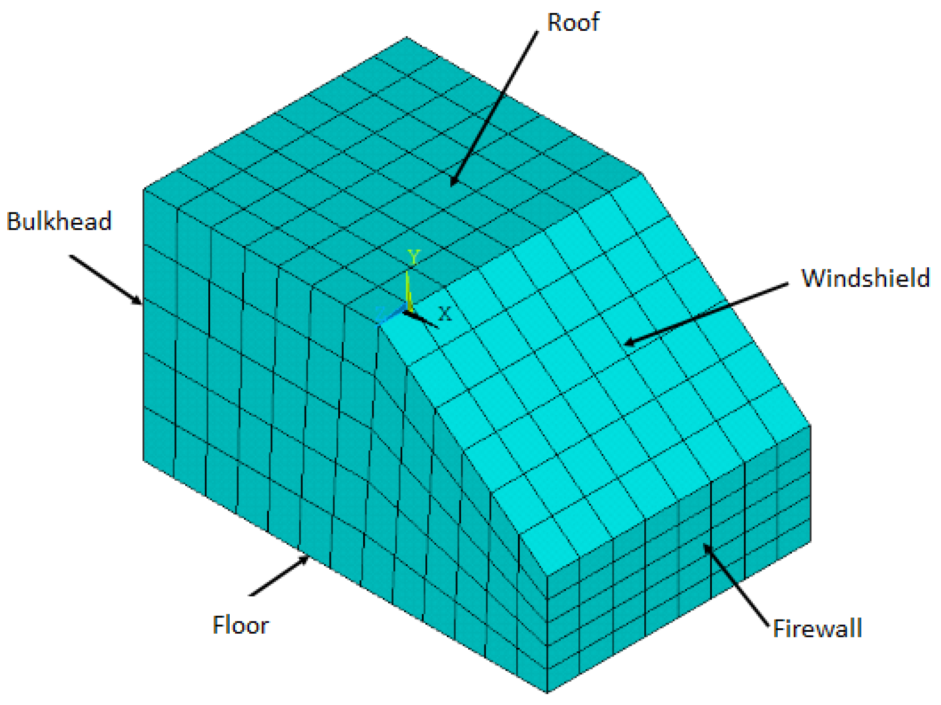
5.2. Simplified Car Interior with Flexible Plates

In this section, we considered a vibro-acoustic finite element model of a simplified automobile passenger compartment. The finite element model presented in Figure 11 was modeled in ANSYS software [11]. For modeling the acoustic cavity, FLUID30 elements were used. These are 3D elements having 8-nodes with 4 degrees of freedom per node: 3 translational displacements in the x, y, and z directions, and a pressure. For structure plates, SHELL181 elements were adopted which are 2D quadrilateral elements. A unit harmonic force in the frequency range 0–500 Hz is applied perpendicularly at the center of the firewall plate. The fluid inside the cabin is the air whose properties are: its density is 1.21 kg/m${}^3$ and the sound speed is 343 m/s.

The material characteristics of the structure are presented in

Table 3. Material properties of the structure.

Structure	Elasticity (Pa)	Poisson’s Ratio	Density (kg/m${}^3$)
Steel	2.1 × 10${}^{11}$	$0.3$	7850
Glass	6.2 × 10${}^{10}$	$0.24$	2300

.

The thickness values of the structural panels are listed in

Table 4. Panel thicknesses.

Panel	Thickness Value (mm)
firewall ($t_1$)	0.8
bulkhead ($t_2$)	0.8
roof ($t_3$)	0.7
floor ($t_4$)	0.9
windshield ($t_5$)	5

.

Table 5. Characteristics of uncertain parameters.

Variables	Mean Value	Cov	Distribution Type
$E_s$ (Pa)	2.1 × 10${}^{11}$	0.05	Normal
$E_g$ (Pa)	6.2 × 10${}^{10}$	0.05	Normal
${\rho }_a$ (kg/m${}^3$)	1.21	0.05	Normal
$t_1$ (mm)	0.8	0.02	Uniform
$t_5$ (mm)	5	0.02	Uniform

presents the different uncertain parameters chosen for this example.

The sound pressure level inside the cavity is approximated using Kriging model. The Kriging estimator is constructed through 50 Latin hypercube sampling points. An additional 50 sampling points are generated in order to validate the efficiency of the surrogate models. The accuracy of the approximation was verified by the cross-validation as shown in Figure 12.

After the validation of the Kriging surrogate model, a sampling set with the number of $N={10}^6$ for uncertain parameters (Table 5) is generated, then the MCS is performed using the Kriging approximation Figure 13.

It is clear that the presence of uncertainties affects the mean of the sound pressure level with small variation. Indeed, the maximum value of the SPL mean at frequency ∼280 Hz increased by $4.8$ dB as shown in Figure 13. It should be noted that the deterministic FEM computing time for one sampling is approximate 10 min. Furthermore, the computational cost of the training points is equal to: $50\times 10=500$ min. So, if the uncertainty analysis is performed using MCS based on FEM, the computational time will be taken about $10\times {10}^6$ min, while the MCS based on Kriging models strongly reduces the computational cost (about 108 s).

6. Conclusions

The aim of this paper is to study the performance of a vibro-acoustic model under the presence of uncertainties in the geometrical and material parameters of the model and to evaluate this performance using Monte Carlo simulations (MCS). The originality of the paper is focused on the implementation of a Kriging meta-model in the uncertainty quantification process which allows to significantly reduce the computational time of Monte Carlo simulations while guaranteeing robust and reliable simulation results. Kriging meta-models are generally subject to numerical problems. Thus, a parametric study was implemented in this work to determine the minimum number of training points that ensures a better fit of the real model. The results show that the Kriging predictor with 30 LHS points for the first application and 50 LHS for the second application provides the best fit compromise of the developed meta-model with the real FEM model. Through the performed analysis, it is clearly proven that the presence of uncertainties has slightly affected the average SPL. Indeed, the maximum value of the average SPL at the frequency 280 Hz increased by 4.8 dB. Overall, the results obtained are both interesting and useful, the developed methodology being able to analyze the influence of model uncertainty on the system response in a satisfactory manner. Therefore, it is also expected to work well with more complicated problems such as industrial vibro-acoustic models (automobile passenger compartment).

References

1. Craggs, A. An acoustic finite element approach for studying boundary flexibility and sound transmission between irregular enclosures. J. Sound Vib. 1973, 30, 343–357. [Google Scholar] [CrossRef]
2. Nefske, D.; Wolf, J., Jr.; Howell, L. Structural-acoustic finite element analysis of the automobile passenger compartment: A review of current practice. J. Sound Vib. 1982, 80, 247–266. [Google Scholar] [CrossRef]
3. Song, C.K.; Hwang, J.K.; Lee, J.M.; Hedrick, J.K. Active vibration control for structural–acoustic coupling system of a 3-D vehicle cabin model. J. Sound Vib. 2003, 267, 851–865. [Google Scholar] [CrossRef]
4. Peretti, L.F.; Dowell, E.H. Asymptotic modal-analysis of a rectangular acoustic cavity excited by wall vibration. AIAA J. 1992, 30, 1991–1998. [Google Scholar] [CrossRef]
5. Sum, K.S.; Pan, J. On acoustic and structural modal cross-couplings in plate-cavity systems. J. Acoust. Soc. Am. 2000, 107, 2021–2038. [Google Scholar] [CrossRef] [PubMed]
6. Redonnet, S.; Cunha, G. An advanced hybrid method for the acoustic prediction. Adv. Eng. Softw. 2015, 88, 30–52. [Google Scholar] [CrossRef]
7. Bös, J. Numerical optimization of the thickness distribution of three-dimensional structures with respect to their structural acoustic properties. Struct. Multidiscip. Optim. 2006, 32, 12–30. [Google Scholar] [CrossRef]
8. Abbes, M.; Bouaziz, S.; Chaari, F.; Maatar, M.; Haddar, M. An acoustic-structural interaction modelling for the evaluation of a gearbox-radiation noise. Int. J. Mech. Sci. 2007, 50, 569–577. [Google Scholar] [CrossRef]
9. Akrout, A.; Karra, C.; Hammami, L.; Haddar, M. Viscothermal fluid effects on vibro-acoustic behaviour of double elastic panels. Int. J. Mech. Sci. 2007, 50, 764–773. [Google Scholar] [CrossRef]
10. Dammak, K.; Koubaa, S.; El hami, A.; Walha, L.; Haddar, M. Numerical modelling of vibro-acoustic problem in presence of uncertainty: Application to a vehicle cabin. Appl. Acoust. 2019, 144, 113–123. [Google Scholar] [CrossRef]
11. Dammak, K.; El Hami, A.; Koubaa, S.; Walha, L.; Haddar, M. Reliability based design optimization of coupled acoustic-structure system using generalized polynomial chaos. Int. J. Mech. Sci. 2017, 134, 75–84. [Google Scholar] [CrossRef]
12. Dammak, K.; Koubaa, S.; El Hami, A.; Walha, L.; Haddar, M. Numerical modeling of uncertainty in acoustic propagation via generalized Polynomial Chaos. J. Theor. Appl. Mech. 2019, 57, 3–15. [Google Scholar] [CrossRef]
13. Sepahvand, K.; Marburg, S. On uncertainty quantification in vibroacoustic problems. In Proceedings of the 9th International Conference on Structural Dynamics, EURODYN, Porto, Portugal, 30 June–2 July 2014. [Google Scholar]
14. Xia, B.; Yin, S.; Yu, D. A new random interval method for response analysis of structural–acoustic system with interval random variables. Appl. Acoust. 2015, 99, 31–42. [Google Scholar] [CrossRef]
15. Hurtado, J.E.; Alvarez, D.A. The encounter of interval and probabilistic approaches to structural reliability at the design point. Comput. Methods Appl. Mech. Engrgy 2012, 225–228, 74–94. [Google Scholar] [CrossRef]
16. Guerine, A.; El Hami, A.; Walha, L.; Fakhfakh, T.; Haddar, M. Dynamic response of a Spur gear system with uncertain friction coefficient. Adv. Eng. Softw. 2016, 120, 45–54. [Google Scholar] [CrossRef]
17. Barillon, F.; Boubaker, M.; Mordillat, P.; Lardeur, P. Vibro-acoustic variability of a body in white using Monte Carlo simulation in a development process. In Proceedings of the Interantional Conference on Noise and Vibraiton Engineering (ISMA), Leuven, Belgium, 17–19 September 2012. [Google Scholar]
18. Durand, J.F.; Gagliardini, L.; Soize, C. Random uncertainties modelling for vibroacoustic frequency response functions of cars. In International Conference on Modal Analysis, Noise and Vibration Engineering; Katholieke Univ Leuven: Leuven, Belgium, 2004; Volume 1, pp. 3255–3266. [Google Scholar]
19. Gagliardini, L.; Durand, J.F.; Soize, C. Stochastic modeling of the vibro-acoustic behavior of production cars. J. Acoust. Soc. Am. 2008, 123, 3533. [Google Scholar] [CrossRef]
20. Fernandez, C.; Soize, C.; Gagliardini, L. Sound-insulation layer modelling in car computational vibroacoustics in the medium-frequency range. Acta Acust. United Acust. 2010, 96, 437–444. [Google Scholar] [CrossRef] [Green Version]
21. Sarkar, A.; Ghanem, R. Mid-frequency structural dynamics with parameter uncertainty. Comput. Methods Appl. Mech. Eng. 2002, 191, 5499–5513. [Google Scholar] [CrossRef]
22. Knio, O.M.; Le Maitre, O. Uncertainty propagation in CFD using polynomial chaos decomposition. Fluid Dyn. Res. 2006, 38, 616. [Google Scholar] [CrossRef]
23. Creamer, D.B. On using polynomial chaos for modeling uncertainty in acoustic propagation. J. Acoust. Soc. Am. 2006, 119, 1979–1994. [Google Scholar] [CrossRef]
24. Sepahvand, K.; Scheffler, M.; Marburg, S. Uncertainty quantification in natural frequencies and radiated acoustic power of composite plates: Analytical and experimental investigation. Appl. Acoust. 2015, 87, 23–29. [Google Scholar] [CrossRef]
25. Forrester, A.; Sobester, A.; Keane, A. Engineering Design via Surrogate Modelling: A Practical Guide; Wiley: New York, NY, USA, 2008. [Google Scholar]
26. Jin, R.; Du, X.; Chen, W. The use of metamodeling techniques for optimization under uncertainty. Struct. Multidiscip. Optim. 2003, 25, 99–116. [Google Scholar] [CrossRef]
27. Dey, S.; Mukhopadhyay, T.; Adhikari, S. Metamodel based high-fidelity stochastic analysis of composite laminates: A concise review with critical comparative assessment. Compos. Struct. 2017, 171, 227–250. [Google Scholar] [CrossRef] [Green Version]
28. Abid, F.; Dammak, K.; El Hami, A.; Merzouki, T.; Trabelsi, H.; Walha, L.; Haddar, M. Surrogate models for uncertainty analysis of micro-actuator. Microsyst. Technol. 2020, 26, 2589–2600. [Google Scholar] [CrossRef]
29. Laurent, L.; Boucard, P.A.; Soulier, B. Generation of a cokriging metamodel using a multiparametric strategy. Comput. Mech. 2013, 51, 151–169. [Google Scholar] [CrossRef] [Green Version]
30. Dammak, K.; El Hami, A. Multi-objective reliability based design optimization using Kriging surrogate model for cementless hip prosthesis. Comput. Methods Biomech. Biomed. Eng. 2020, 23, 854–867. [Google Scholar] [CrossRef]
31. Debich, B.; Yaich, A.; Dammak, K.; El Hami, A.; Gafsi, W.; Walha, L.; Haddar, M. Integration of multi-objective reliability-based design optimization into thermal energy management: Application on phase change material-based heat sinks. J. Energy Storage 2021, 41, 102906. [Google Scholar] [CrossRef]
32. Simpson, T.; Peplinski, J.; Koch, P.; Allen, J. On the use of statistics in design and the implications for deterministic computer experiments. In Proceedings of the International Design Engineering Technical Conferences and Computers and Information in Engineering Conference, Sacramento, CA, USA, 14–17 September 1997. [Google Scholar]
33. Myers, R.; Montgomery, D. Response Surface Methodology, 2nd ed.; Wiley: New York, NY, USA, 2002. [Google Scholar]
34. Kurtaran, H.; Eskandarian, A.; Marzougui, D.; Bedewi, N.E. Crashworthiness design optimization using successive response surface approximations. Comput. Mech. 2002, 29, 409–421. [Google Scholar] [CrossRef]
35. Dey, S.; Mukhopadhyay, T.; Khodaparast, H.H.; Kerfriden, P.; Adhikari, S. Rotational and ply-level uncertainty in response of composite shallow conical shells. Compos. Struct. 2015, 131, 594–605. [Google Scholar] [CrossRef] [Green Version]
36. Janusevskis, J.; Le Riche, R. Simultaneous kriging-based estimation and optimization of mean response. J. Glob. Optim. 2013, 55, 313–336. [Google Scholar] [CrossRef]
37. Mukhopadhyay, T.; Chakraborty, S.; Dey, S.; Adhikari, S.; Chowdhury, R. A critical assessment of Kriging model variants for high-fidelity uncertainty quantification in dynamics of composite shells. Arch. Comput. Methods Eng. 2017, 24, 495–518. [Google Scholar] [CrossRef]
38. Dammak, K.; El Hami, A. Thermal reliability-based design optimization using Kriging model of PCM based pin fin heat sink. Int. J. Heat Mass Transf. 2021, 166, 120745. [Google Scholar] [CrossRef]
39. Miriyala, S.S.; Mittal, P.; Majumdar, S.; Mitra, K. Comparative study of surrogate approaches while optimizing computationally expensive reaction networks. Chem. Eng. Sci. 2016, 140, 44–61. [Google Scholar] [CrossRef]
40. Miriyala, S.S.; Subramanian, V.R.; Mitra, K. TRANSFORM-ANN for online optimization of complex industrial processes: Casting process as case study. Eur. J. Oper. Res. 2018, 264, 294–309. [Google Scholar] [CrossRef]
41. Kinsler, L.; Frey, A. Fundamental of Acoustics; John Wiley & SonsNew: New York, NY, USA, 1962. [Google Scholar]
42. Morse, P.; Ingardku. Theoretical Acoustics; McGraw-Hill Book Company: New York, NY, USA, 1968. [Google Scholar]
43. Larbi, W.; Deü, J.; Ohayon, R. Vibroacoustic analysis of double-wall sandwich panels with viscoelastic core. Comput. Struct. 2016, 174, 92–103. [Google Scholar] [CrossRef]
44. Lupea, I.; Szatmari, R. Vibroacoustic Frequency Response on a Passenger Compartment. J. Vibroeng. 2010, 4, 406–418. [Google Scholar]
45. McKay, M.; Beckman, R.; Conover, W. A Comparison of Three Methods for Selecting Values of Input Variables in the Analysis of Output from a Computer Code. Technometrics 1979, 21, 239–245. [Google Scholar]
46. Stander, N.; Roux, W.; Goel, T.; Eggleston, T.; Craig, K. LS-Opt User’s Manual; Technical Report; Livermore Software Technology Corporation: Livermore, CA, USA, 2010. [Google Scholar]
47. Ryberg, A.; Domeij, B.; Nilsson, L. Metamodel-Based Multidisciplinary Design Optimization for Automotive Applications; Technical Report; Linköping University, Division of Solid Mechanics: Linköping, Sweden, 2012. [Google Scholar]
48. Meckesheimer, M.; Booker, A.; Barton, R.; Simpson, T. Computationally inexpensive metamodel assessment strategies. AIAA J. 2002, 40, 2053–2060. [Google Scholar] [CrossRef]
49. Forrester, A.I.; Keane, A.J. Recent advances in surrogate-based optimization. Prog. Aerosp. Sci. 2009, 45, 50–79. [Google Scholar] [CrossRef]
50. Xia, B.; Yu, D. Optimization based on reliability and confidence interval design for the structural-acoustic system with interval probabilistic variables. J. Sound Vib. 2015, 336, 1–15. [Google Scholar] [CrossRef]
51. Nielsen, H.; Lophaven, S.; Søndergaard, J.; Dace, A. A Matlab Kriging Toolbox; Technical Report; Technical University of Denmark: Kongens Lyngby, Denmark, 2002. [Google Scholar]
Figure 1. Boundary conditions of the vibro-acoustic system.
Applsci 12 01503 g001
Figure 2. Flowchart of the MCS.
Applsci 12 01503 g002
Figure 3. Flowchart of surrogate models construction.
Applsci 12 01503 g003
Figure 4. Acoustic-structural model.
Applsci 12 01503 g004
Figure 5. 3D finite element model.
Applsci 12 01503 g005
Figure 6. Sound pressure level inside the acoustic cavity.
Applsci 12 01503 g006
Figure 7. Cross-validation results of Kriging for maximum SPL with 20 LHS points.
Applsci 12 01503 g007
Figure 8. Cross-validation results of Kriging for maximum SPL with 30 LHS points.
Applsci 12 01503 g008
Figure 9. Mean value of the SPL.
Applsci 12 01503 g009
Figure 10. Standard deviation value of the SPL.
Applsci 12 01503 g010
Figure 11. 3D model of the passenger cavity.
Applsci 12 01503 g011
Figure 12. Cross-validation results for SPL using Kriging.
Applsci 12 01503 g012
Figure 13. Variation of the SPL mean with the frequency.
Applsci 12 01503 g013