
Pressure Drop and Particle Settlement of Gas–Solid Two-Phase Flow in a Pipe

Abstract
:1. Introduction
2. Basic Equations
3. Numerical Simulation
3.1. Parameters
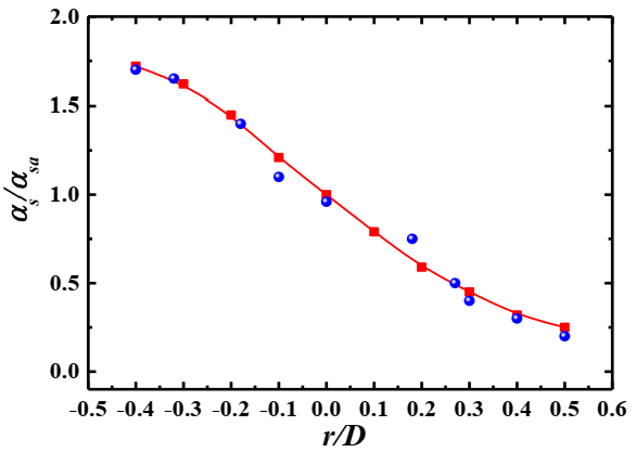
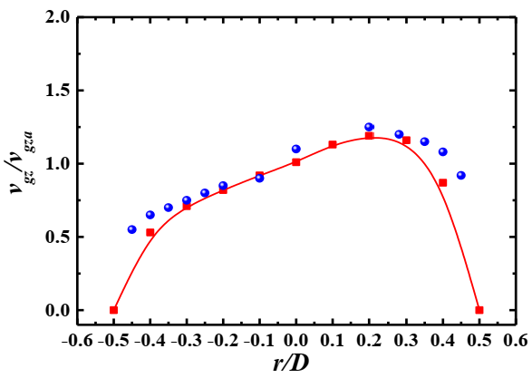
3.2. Validation
4. Results and Discussion
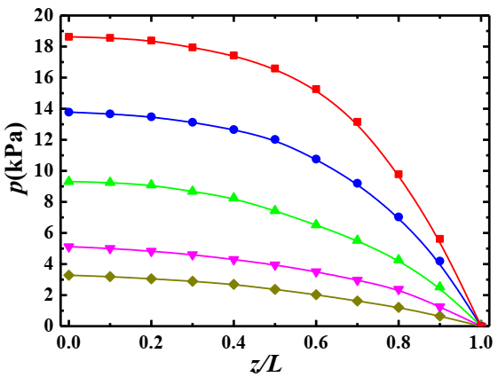
4.1. Distribution of Pressure along the Flow Direction
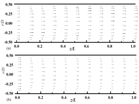
4.2. Distribution of Velocity along the Flow Direction
4.3. Distribution of Particle Volume Concentration
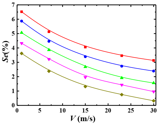
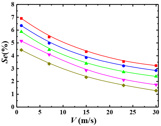
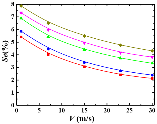
4.4. Relationship between the Settlement Index and Mixture Inlet Velocity
4.4.1. Effect of Particle Volume Concentration
4.4.2. Effect of Particle Mass Flow
4.4.3. Effect of Particle Diameter
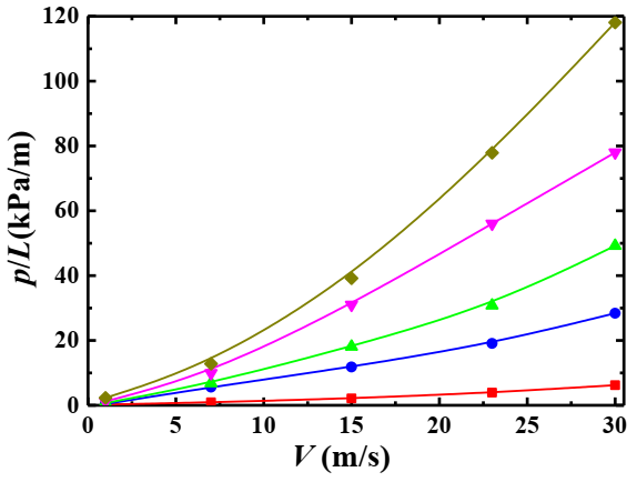
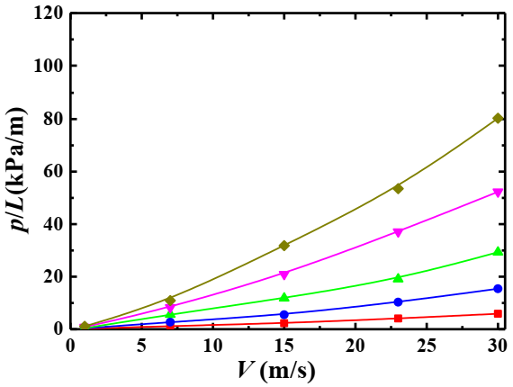
4.5. Relationship between the Pressure Drop and Mixture Inlet Velocity
4.5.1. Effect of Particle Volume Concentration
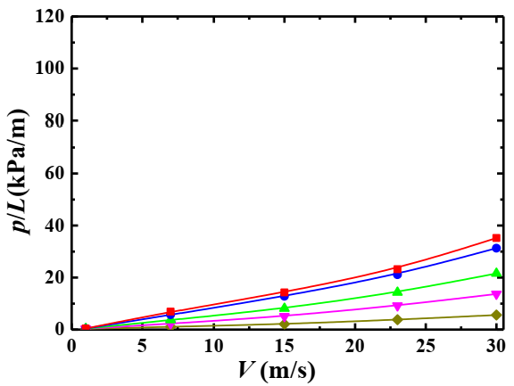
4.5.2. Effect of Particle Mass Flow
4.5.3. Effect of Particle Diameter
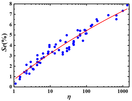
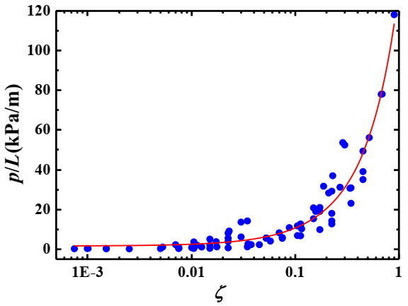
4.6. Relationship of Settlement Index, Pressure Drop and Related Parameters
5. Conclusions
Author Contributions
Funding
Conflicts of Interest
References
- Sergeev, V.; Vatin, N.; Kotov, E.; Nemova, D.; Khorobrov, S. Slug regime transitions in a two-phase flow in horizontal round pipe. CFD simulations. Appl. Sci. 2020, 23, 8739. [Google Scholar] [CrossRef]
- Nie, D.M.; Lin, J.Z. A LB-DF/FD Method for particle suspensions. Commun. Comput. Phys. 2010, 7, 544–563. [Google Scholar]
- Jin, Y.; Lu, H.; Guo, X.; Gong, X. Flow patterns classification of dense-phase pneumatic conveying of pulverized coal in the industrial vertical pipeline. Adv. Powder Technol. 2019, 30, 1277–1289. [Google Scholar] [CrossRef]
- Lin, J.Z.; Qian, L.J.; Xiong, H.B. Effects of operating conditions on the droplet deposition onto surface in the atomization impinging spray with an impinging plate. Surf. Coat. Technol. 2009, 203, 1733–1740. [Google Scholar] [CrossRef]
- Tong, Z.H.; Liu, H.T.; Chang, J.Z.; An, K. Direct simulation of melting solid particles sedimentation in a Newtonian fluid. Acta Phys. Sin. 2012, 61, 024401. [Google Scholar] [CrossRef]
- Balakin, B.; Hoffmann, A.C.; Kosinski, P.; Rhyne, L.D. Eulerian-Eulerian CFD model for the sedimentation of spherical particles in suspension with high particle concentrations. Eng. Appl. Comput. Fluid Mech. 2010, 4, 116–126. [Google Scholar] [CrossRef] [Green Version]
- Tao, S.; Guo, Z.L.; Wang, L. P Numerical study on the sedimentation of single and multiple slippery particles in a Newtonian fluid. Powder Technol. 2017, 315, 126–138. [Google Scholar] [CrossRef] [Green Version]
- Chiodi, F.; Claudin, P.; Andreotti, B. A two-phase flow model of sediment transport: Transition from bedload to suspended load. J. Fluid Mech. 2014, 755, 561–581. [Google Scholar] [CrossRef] [Green Version]
- Senapati, S.K.; Dash, S.K. Computation of pressure drop and heat transfer in gas-solid suspension with small sized particles in a horizontal pipe. Part. Sci. Technol. 2019, 38, 985–998. [Google Scholar] [CrossRef]
- Naveh, R.; Tripathi, N.M.; Kalman, H. Experimental pressure drop analysis for horizontal dilute phase particle- fluid flows. Powder Technol. 2017, 321, 355–368. [Google Scholar] [CrossRef]
- Ariyaratne, W.; Ratnayake, C.; Melaaen, M. CFD modeling of dilute phase pneumatic conveying in a horizontal pipe using Euler-Euler approach. Part. Sci. Technol. 2019, 37, 1011–1019. [Google Scholar] [CrossRef]
- Narimatsu, C.; Ferreira, M. Vertical pneumatic conveying in dilute and dense-phase flows: Experimental study of the influence of particle density and diameter on fluid dynamic behavior. Braz. J. Chem. Eng. 2001, 18, 221–232. [Google Scholar] [CrossRef]
- Herbreteau, C.; Bouard, R. Experimental study of parameters which influence the energy minimum in horizontal gas-solid conveying. Powder Technol. 2000, 112, 213–220. [Google Scholar] [CrossRef]
- Levy, A. Two-fluid approach for plug flow simulations in horizontal pneumatic conveying. Powder Technol. 2000, 112, 263–272. [Google Scholar] [CrossRef]
- Levy, A.; Mooney, T.; Marjanovic, P.; Mason, D.J. A comparison of analytical and numerical models for gas-solid flow through straight pipe of different inclinations with experimental data. Powder Technol. 1997, 93, 253–260. [Google Scholar] [CrossRef]
- Benyahia, S.; Arastoopour, H.; Knowlton, T.M.; Massah, H. Simulation of particles and gas flow behavior in the riser section of a circulating fluidized bed using the kinetic theory approach for the particulate phase. Powder Technol. 2000, 112, 24–33. [Google Scholar] [CrossRef]
- Tsuji, Y.; Morlkawa, Y.; Tanaka, T.; Nakatsukasa, N.; Nakatani, M. Numerical simulation of gas-solid two phase flow in a two-dimensional horizontal channel. Int. J. Multiph. Flow 1987, 13, 671–692. [Google Scholar] [CrossRef]


| r × θ × S | ∆p/L | r × θ × S | ∆p/L | r × θ × S | ∆p/L |
|---|---|---|---|---|---|
| 24 × 32 × 208 | 50,891 | 32 × 24 × 208 | 50,889 | 32 × 32 × 192 | 50,893 |
| 28 × 32 × 208 | 50,880 | 32 × 28 × 208 | 50,879 | 32 × 32 × 200 | 50,881 |
| 32 × 32 × 208 | 50,872 | 32 × 32 × 208 | 50,872 | 32 × 32 × 208 | 50,872 |
| 36 × 32 × 208 | 50,868 | 32 × 36 × 208 | 50,869 | 32 × 32 × 216 | 50,867 |
| 40 × 32 × 208 | 50,865 | 32 × 40 × 208 | 50,867 | 32 × 32 × 224 | 50,864 |
Publisher’s Note: MDPI stays neutral with regard to jurisdictional claims in published maps and institutional affiliations. |
© 2022 by the authors. Licensee MDPI, Basel, Switzerland. This article is an open access article distributed under the terms and conditions of the Creative Commons Attribution (CC BY) license (https://creativecommons.org/licenses/by/4.0/).
Share and Cite
Lin, W.; Li, L.; Wang, Y. Pressure Drop and Particle Settlement of Gas–Solid Two-Phase Flow in a Pipe. Appl. Sci. 2022, 12, 1623. https://doi.org/10.3390/app12031623
Lin W, Li L, Wang Y. Pressure Drop and Particle Settlement of Gas–Solid Two-Phase Flow in a Pipe. Applied Sciences. 2022; 12(3):1623. https://doi.org/10.3390/app12031623
Chicago/Turabian StyleLin, Wenqian, Liang Li, and Yelong Wang. 2022. "Pressure Drop and Particle Settlement of Gas–Solid Two-Phase Flow in a Pipe" Applied Sciences 12, no. 3: 1623. https://doi.org/10.3390/app12031623