Application of a Musical Robot for Adjusting Guitar String Re-Excitation Parameters in Sound Synthesis

Abstract

Sound synthesis methods based on physical modelling of acoustic instruments depend on data that require measurements and recordings. If a musical instrument is operated by a human, a difficulty in filtering out variability is introduced due to a lack of repeatability in excitation parameters, or in varying physical contact between a musician and an instrument, resulting in the damping of vibrating elements. Musical robots can solve this problem. Their repeatability and controllability allows studying even subtle phenomena. This paper presents an application of a robot in studying the re-excitation of a string in an acoustic guitar. The obtained results are used to improve a simple synthesis model of a vibrating string, based on the finite difference method. The improved model reproduced the observed phenomena, such as the alteration of the signal spectrum, damping, and ringing, all of which can be perceived by a human, and add up to the final sound of an instrument. Moreover, as it was demonstrated by using two different string plucking mechanisms, musical robots can be redesigned to study other sound production phenomena and, thus, to further improve the behaviours of and sounds produced by models applied in sound synthesis.

1. Introduction

Among the various methods of sound synthesis applied for musical purposes, one of the most powerful and versatile is based on numerical modelling of actual musical instruments [1,2]. Such method is commonly referred to as physical modelling sound synthesis, and is often implemented on the basis of finite difference simulations [1], waveguides [3,4,5,6,7], or modal techniques [8]. While, in general, sound synthesis aims at the sound itself, and its parameters are related to acoustic signal or its underlying abstract model, in physical modelling synthesis, parameters have actual physical counterparts, related mostly to the geometry and material of the object in question, or to the excitation of its vibrating elements. Therefore, in order to design a proper model, a real acoustic instrument needs to be studied and measured, so that the relevant effects can be reproduced, and the model can behave plausibly. However, it is important to note that, due to requirement of operating and controlling the model in real time, sound synthesis has to trade accuracy for computational efficiency. Simplifications are common, yet, still, important instrument features need to be considered. Some instruments, such as the grand piano, have been studied relatively well, to the level of subtle effects such as unison impact, inharmonicity, double decay, or reexcitation [9,10,11]. However, there is less data regarding some of the more subtle effects for the acoustic guitar, probably due to lack of appropriate test stands, in which a guitar could be mounted in a stable way, and excited in a repeatable, controllable manner.

This paper presents a test stand and measurements aimed at reproducing the effect of a guitar string re-excitation, i.e., plucking a vibrating string. The effect is clearly perceivable in the temporal and spectral domains, making subsequent plucks less repeatable, and as such shall be replicated in sound synthesis. There are studies regarding other guitar string excitation phenomena, such as plucking angle [12] or double decay [13], where a variety of plucking mechanisms are employed. However, studying re-excitation has very specific requirements. The plucking mechanism needs to be repeatable with regard to plucking amplitude. Moreover, it has to be able to perform multiple plucks, with precisely set and possibly adjustable re-excitation delay. Such requirements are far beyond the capabilities of human operators. Therefore, this study explores the use of a robot. The robot has been previously tested for the stability of its plucking amplitude [14], and has been recently expanded with a module able to perform a double pluck with a delay as short as the fundamental period of the lowest guitar string.

In our study a test stand equipped with a guitar-plucking robot has been employed to observe the effect of string re-excitation in order to improve computational models of the instruments utilised in sound synthesis. Initially, a basic model of a plucked string has been implemented using the finite difference method [1,15]. Re-excitation has been modelled by applying initial conditions twice, separated with adjustable time intervals. Two series of simulations have been carried out, with parameters reflecting the configurations of the test stand with two different plucking mechanisms, characterised by short and long re-excitation delay. Next, the robot has been used to pluck the string with both mechanisms. The results of measurements and simulations have been analysed and compared. A distinct effect of contact between the vibrating string and the moving plectrum, just before the re-excitation, has been observed in a real instrument. A modified model has been designed to reproduce this behaviour and the parameters of the simulated effect have been adjusted to match the real phenomenon.

According to our knowledge, application of a robot to control and study an instrument as a way to improve the latter’s sound synthesis model is a novel approach, with great potential. Even though both the stand and the model require further improvement, the use of a robot has already proved to be advantageous, allowing experiments to be easily repeated and adjusted.

2. Methods

2.1. Test Stand

For the needs of the research described in this article, a test stand was created using a three-axis, Cartesian robot (Figure 1) equipped with a replaceable end-of-arm tooling (EOAT) adapted to excite an acoustic guitar string. The use of the robot was dictated by the need to obtain repeatability in certain parameters: the point of the string’s excitation, the strength of the attack on the string, and the duration of the mechanism’s operations. The displacements in the x and z axes were driven by stepper motors, and the linear motion systems were built on the basis of a V-Slot aluminum profile system and trapezoidal lead screws, which guaranteed the desired precision of the mechanism. The y-axis position was fixed for the purpose of the experiment.

Two sets of end effectors were used for the experiment purposes (Figure 2). The first one’s (Figure 2a) task was to simulate the string excitation process of a human playing the guitar, with some assumed simplifications. The plucking element used in the tool was a standard Dunlop Tortex Sharp guitar pick, 0.73 mm thick. In order to eliminate the undesirable stiffness in the coupling of the plectrum with the end effector’s housing, a damping material in the form of a rubber pad was used, imitating the effect of a human finger holding the guitar pick.

In the process of string excitation, the musical robot performed a movement in two axes, x and z (Figure 3). The movement in the z axis caused the pick to attack the guitar string and was also used to return the EOAT to the starting position. The movement in the x axis was used to bypass the string as the end effector returned to the starting position. The movement pattern was dictated by the need to excite the string from the same direction, and it was carried out in the sequence illustrated in the Figure 3.

The implemented robot motion allowed achieving the time of a single string excitation cycle of over 500 ms. The discrepancies in the execution time of individual cycles—at the level of about $6\%$—resulted from the lack of real-time support by the operating system used to control the robot.

The second end effector (Figure 2b) used in the robot was designed to achieve re-excitation of the string for much shorter time courses. This was achieved by creating a set of disks (Figure 4) with protruding elements placed at certain angles to each other. The circles were mounted on a continuous rotation servo motor actuator. The diameter of the prepared discs was 11 mm, while the excitation protrusions were extended to a length of 1 mm outside the circle area. The dimensions of the disks were dictated by the parameters of the servo motor used for their rotation.

Figure 4a,b shows the models of the two discs used in the study. The segments highlighted in the pictures represent the axes of symmetry of the protrusions. The $\left|AB\right|$ and $|A{B}^{\prime }|$ segments correspond to the axes of symmetry arrangement for the disk in Figure 4a, arranged at an angle of $\alpha =5.2^{\circ }$. Such an arrangement of the plectrums allowed to achieve re-excitation after approx. 12 ms. The $\left|AB\right|$ and $|A{B}_1^{\prime }|$ segments correspond to the axes arrangement for the disk from the Figure 4b, arranged at an angle of $\beta ={26}^{\circ }$ which allowed for re-excitation after approx. 70 ms. The presented disks were printed with DLP technology using reinforced resin, which limited the wear of the string excitation protrusions.

2.2. Sound Synthesis

A finite difference (FD) method has been applied to simulate the plucked string. It is simple enough to operate in real time, as well as to simultaneously produce output signal and react to control. Therefore it is possible to play such a simulated instrument, and control it while it sounds, just like its acoustic counterpart. The FD method is flexible enough to allow various modifications of the basic model.

The model is based on a partial differential equation proposed in a work of Bensa et al. [16]. It is a wave equation with added stiffness, and frequency-dependent losses:

$${\displaystyle \frac{{\partial }^{2}u}{\partial t^2}}={\gamma }^2{\displaystyle \frac{{\partial }^{2}u}{\partial x^2}}-{\kappa }^2{\displaystyle \frac{{\partial }^{4}u}{\partial x^4}}-2{\sigma }_0{\displaystyle \frac{\partial u}{\partial t}}+2{\sigma }_1{\displaystyle \frac{{\partial }^{3}u}{\partial t\partial x^2}}$$

(1)

The equation is given in variables scaled to the length of a string L:

$$x={\displaystyle \frac{\tilde{x}}{L}}\gamma ={\displaystyle \frac{c}{L}}$$

(2)

The stiffness parameter is defined as [1,17]:

$$\kappa =\sqrt{{\displaystyle \frac{EI}{\rho A{L}^4}}}$$

(3)

where $\tilde{x}$—dimensional coordinate, c—transverse wave velocity, L—string length E—Young’s modulus, I—moment of inertia, $\rho$—material density, A—area of cross-section.

Losses increase with frequency and are determined by two decay times, $T_{60}$, specified for the frequencies $f_1<f_2$ [1]:

$$\begin{array}{cc}\hfill {\sigma }_0& =\frac{6ln\left(10\right)}{\xi \left(f_2\right)-\xi \left(f_1\right)}\left({\displaystyle \frac{\xi \left(f_2\right)}{T_{60}\left(f_1\right)}}-{\displaystyle \frac{\xi \left(f_1\right)}{T_{60}\left(f_2\right)}}\right)\hfill \\ \hfill {\sigma }_1& ={\displaystyle \frac{6ln\left(10\right)}{\xi \left(f_2\right)-\xi \left(f_1\right)}}\left(-{\displaystyle \frac{1}{T_{60}\left(f_1\right)}}+\frac{1}{T_{60}\left(f_2\right)}\right)\hfill \end{array}$$

(4)

with:

$$\xi \left(f\right)={\displaystyle \frac{-{\gamma }^2+\sqrt{{\gamma }^4+16{\kappa }^2{\pi }^2{f}^2}}{2{\kappa }^2}}$$

(5)

The equation is solved using an explicit differential scheme, proposed by Bilbao [1]:

$${\delta }_{tt}{u}_l\left[n\right]={\gamma }^2{\delta }_{xx}{u}_l\left[n\right]-{\kappa }^2{\delta }_{xxxx}{u}_l\left[n\right]-2{\sigma }_0{\delta }_{t·}{u}_l\left[n\right]+2{\sigma }_1{\delta }_{t-}{\delta }_{xx}{u}_l\left[n\right]$$

(6)

with a Courant–Friedrichs–Lewy (CFL) stability condition, where n is the time index, l the spatial grid index, and $\delta$ symbols represent derivative operators. The temporal operators are defined as:

$$\begin{array}{cc}\hfill & {\delta }_{t-}={\displaystyle \frac{1}{T}}(1-e_{t-})\cong {\displaystyle \frac{\partial }{\partial t}}\hfill \\ \hfill & {\delta }_{t·}={\displaystyle \frac{1}{2T}}(e_{t+}-e_{t-})\cong {\displaystyle \frac{\partial }{\partial t}}\hfill \\ \hfill & {\delta }_{tt}={\displaystyle \frac{1}{T^2}}(e_{t+}-2+e_{t-})\cong {\displaystyle \frac{{\partial }^2}{\partial t^2}}\hfill \end{array}$$

(7)

where T is the sampling period. The spatial operators are defined as:

$$\begin{array}{cc}\hfill & {\delta }_{xx}={\displaystyle \frac{1}{X^2}}(e_{x+}-2+e_{x-})\cong {\displaystyle \frac{{\partial }^2}{\partial x^2}}\hfill \\ \hfill & {\delta }_{xxxx}={\displaystyle \frac{1}{X^4}}(e_{x+}{e}_{x+}-4e_{x+}+6-4e_{x-}+e_{x-}{e}_{x-})\cong {\displaystyle \frac{{\partial }^4}{\partial x^4}}\hfill \end{array}$$

(8)

where X is the spatial sampling interval. Definitions (7) and (8) use forward and backward, and the temporal and spatial shift operators:

$$\begin{array}{cc}\hfill & e_{t+}u\left[n\right]=u[n+1]\hfill \\ \hfill & e_{t-}u\left[n\right]=u[n-1]\hfill \\ \hfill & e_{x+}{u}_l\left[n\right]=u_{l+1}\left[n\right]\hfill \\ \hfill & e_{x-}{u}_l\left[n\right]=u_{l-1}\left[n\right]\hfill \end{array}$$

(9)

Dirichlet boundary conditions are applied on both ends of string. Initial conditions are simulated with an idealised pluck, where initial velocity is set to zero, and initial displacement is set according to either raised cosine:

$$c_{rc}\left(x\right)=\left\{\begin{array}{cc}{\displaystyle \frac{c_0}{2}}\left(1+cos\left({\displaystyle \frac{\pi (x-x_0)}{x_{hw}}}\right)\right)& |x-x_0|\le x_{hw}\hfill \\ 0& |x-x_0|>x_{hw}\hfill \end{array}\right.$$

(10)

or the triangular spatial distribution:

$$c_{tri}\left(x\right)=\left\{\begin{array}{cc}{\displaystyle \frac{c_0}{x_0}}x& 0\le x\le x_0\hfill \\ {\displaystyle \frac{c_0}{x_0-1}}(x-1)& x_0<x\le 1\hfill \end{array}\right.$$

(11)

The output signal is read directly from the string displacement, u, using the following linear interpolation operator:

$$I_1\left(x_o\right)u_l=(1-{\alpha }_o)u_{l_o}+{\alpha }_o{u}_{l_o+1}$$

(12)

where ${\alpha }_o$ is the remainder of truncation, X is the spatial sampling interval, $l_o=⌊{\displaystyle \frac{x_o}{X}}⌋$:

$${\alpha }_o={\displaystyle \frac{x_o}{X}}-l_o$$

(13)

so that the readout position can be set to any location on the string, even between grid points.

2.3. Robot-Assisted Measurements

Two attempts at robot-assisted measurements were carried out, as described in

Table 1. Description of robot-assisted experiments with symbols representing them for brevity in the following sections.

Symbol	Plucking Mechanism	Re-Excitation Delay
M1	end effector with a plectrum (slow)	10 values between 544.9 ms and 577.0 ms
M2	EOAT (fast)	2 values: 12 ms and 70 ms

. In the first one (M1) the robot with plectrum-equipped end effector (Figure 2a) performed series of ten, single excitations and ten double excitations with re-excitation delay limited by the mechanism, varying from 544.9 ms to 577.0 ms—the delay was not precisely repeatable. In the second attempt (M2) the robot was equipped with a fast EOAT mechanism (Figure 2b). It performed a series of 10 single excitations, and two series of quick re-excitations, with delays of 12 ms and 70 ms. In all cases, the robot excited the lowest string, E2, which had a fundamental frequency of 82.4 Hz. All the sound recordings were carried out using a Studio Projects C4 condenser microphone.

2.4. Simulations

Four series of simulations with two different models have been carried out, as described in

Table 2. Description of simulations variants with symbols representing them for brevity in the following sections.

Symbol	Model	Re-Excitation Delay
L1	basic	10 equally spaced values between 544.9 ms and 557.1 ms
S1	basic	2 values: 12 ms and 70 ms
L2	improved	10 equally spaced values between 544.9 ms and 557.1 ms
S2	improved	2 values: 12 ms and 70 ms

. Both models are based on a sound synthesis technique discussed in Section 2.2 and a differential scheme given in (6). Simulation parameters have been set to replicate configuration of the robot test stand. They are presented in

Table 3. Simulation parameters; positions are scaled to the length of the string, as in (2).

Parameter	Symbol	Value
sample rate		88,200 Hz
excitation position		0.1899
initial displacement	u0	0.7
initial velocity	v0	0.0
readout position		0.239
fundamental frequency	f0	82.4 Hz
wave equation free parameter	$\gamma$	$2f_0$
inharmonicity	$\kappa$	$\sqrt{0.00001}\gamma /\pi$

.

The first two series of simulations (variants L1 and S1) had been carried out prior to robot-assisted measurements, as a reference. They apply a basic model where both excitation and re-excitation are simulated using the same initial conditions—an additive pluck approximated with raised cosine spatial distribution, defined in (10).

The remaining series (variants L2 and S2) have been carried out after analysing the results of robot-assisted measurements, and represent an improved model. The changes include triangular spatial distribution, as defined in (11), and plucking element behaving, such as a moving string damper in a form of one-sided, rigid non-linearity. Movement velocity and range were adjusted to obtain the effect similar to the one observed in measurements.

In order to replicate behaviour of both plucking mechanisms, simulations have been carried out with long (variants L1 and L2: 10 values between 544.9 ms and 557.1 ms, over one fundamental string period) and short (variants S1 and S2: 12 ms and 70 ms) re-exitation delays. L1 and L2 are compared, using measurements M1, S1, and S2, with M2.

3. Results

3.1. Re-Excitation Visualisation

Figure 5 and Figure 6 present visualisations of the string displacement, u, for simulations L1 and L2. Separate subplots demonstrate the differences caused by delay increasing over one fundamental string period, from 544.9 ms to 557.1 ms. The plots show that, by controlling re-excitation delay, one can significantly alter the character of string vibrations, depending on phase of the excited string section at the moment of re-excitation. However, the simple model (Figure 5) is almost perfectly repeatable over a single string’s period. This behaviour changes in the improved model (Figure 6) due to distortions introduced by prior contact between string and plectrum. In the improved model it would be impossible to cancel out string vibrations simply by choosing appropriate moment, amplitude, and location of re-excitation, because of their much more complex character, caused by contact-induced damping.

3.2. Slow Re-Excitation

Comparative spectra for cases of slow re-excitation are presented in Figure 7, Figure 8 and Figure 9, for robot measurements (M1), and the simple (L1) and improved simulations (L2), respectively. Separate subplots demonstrate differences caused by delay increasing over one fundamental string period, from 544.9 ms to 557.1 ms in Figure 8 and Figure 9, or over all measured delays in Figure 7. Frequency range has been limited to 1400 Hz, sufficient to display first 16 harmonics, while maintaining clarity of presentation. Spectral changes between the first excitation and re-excitation ($\mathrm{\Delta }$) are related to the alteration of sound timbre.

3.3. Fast Re-Excitation

Figure 10 shows a grid of plots presenting the spectra of a single excitation and re-excitation with two delay values (12 ms and 70 ms), for robot measurements (M2) and both simulations (S1 and S2). The robot measurements have been averaged over 10 subsequent cases of excitation or re-excitation. In Figure 11 the same data has been presented as differences between re-excitation spectra and single excitation spectra.

3.4. Time–Frequency Analysis

Figure 12 contains three spectrograms for cases of slow re-excitation (544.9 ms delay). The second excitation is visible around 0.55 s. The robot’s measurement, in the top plot (M1), is compared with the simple model (middle plot—L1) and the improved model (bottom plot—L2). Both spectral and temporal phenomena are noticeable. Temporal resolution is limited in order to maintain the visibility of the individual harmonics on the frequency axis.

4. Discussion

Measurements carried out using a robot-equipped stand supported the claim that the re-excitation of a guitar string produces a sound that is different from a single excitation, or its first excitation. The observed changes in spectra (Figure 11) exceeded 10 dB in some frequency bands, which was clearly perceivable by the human ear [18,19]. The spectral changes depend on the re-excitation delay (Figure 7), so a series of otherwise-similar guitar string plucks (with regards to plucking position, angle, or amplitude) will vary due to the state of the string at the moment of plucking, and this variability can be detected by human hearing. For better realism, sound synthesis needs to replicate this behaviour.

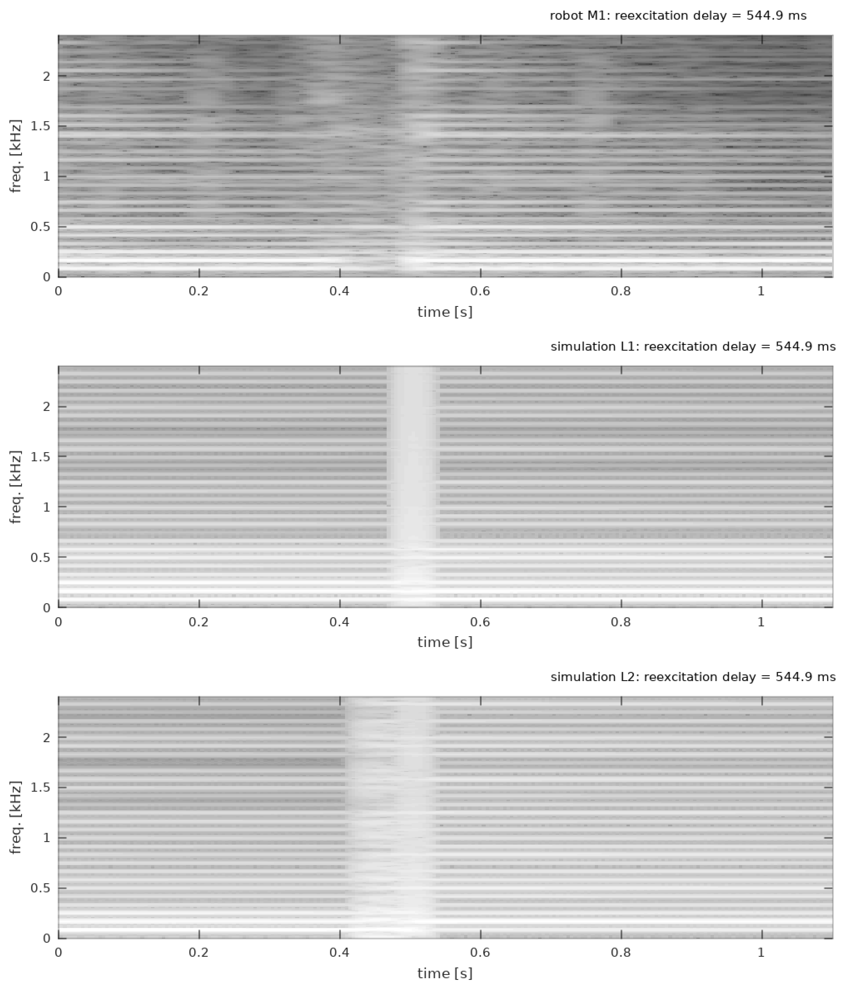
The first simulation model (L1 and S1) took into consideration the fact that a string is vibrating during re-excitation and that secondary excitation is imposed on that state. Apart from that, no previous contact with the plectrum nearing a string was considered. However, the spectrogram of the robot measurement (Figure 12) showed that, just before the re-excitation, the string received partial contact with the moving plectrum, producing two auditory effects: ringing and damping. The latter could be observed by the harmonics becoming less distinct and by so-called pitch-glides—slight and gradual frequency changes in some harmonics. Therefore, the first model was insufficient to replicate these phenomena. What was also interesting is that re-excitation after a single fundamental string period (12 ms) did not produce the same spectrum, contrary to the prediction of the simple model (Figure 10 and Figure 11). The spectral changes caused by re-excitation were larger and more complex, and required a better model to be at least partially reproduced.

The second simulation model (L2 and S2) introduced contact between a plucking element and the string when the former neared the latter before its re-excitation. Spectrogram (Figure 12) shows that it allowed replicating both ringing and damping—the harmonics became less distinct and pitch glides appeared. Moreover, such model predicted the fact that, even after a full fundamental string period, the signal spectrum did not return to its previous state, and some changes remained (Figure 11). Further improvements to the model are possible [20,21,22,23].

Neither of the models was able to predict the actual measured spectra accurately. However, compared with the first model, the second one, at least, predicted the fact that the spectrum actually changed after a full string period (case of 12 ms in Figure 11). One can also observe a weak similarity in a spectral dip around 400 Hz between M1 and S2 in the same plot. In the case of a 70-ms delay (bottom plot in Figure 11) both models predicted spectral changes, but the improved model was able to slightly better reflect some details, such as peaks in the low-frequency range, around 220 Hz, 310 Hz, or 710 Hz, and, again, the area around 400 Hz. For better spectral behaviour, the model would need to consider more than a string, as some phenomena are located in the soundboard [19,24].

Furthermore, the results were very sensitive to even small changes in simulation parameters, such as plectrum movement velocity, plucking position, plucking element profile, or material parameters. In order to closely reproduce a particular instrument, careful measurements need to be considered to precisely estimate values of these parameters. This could be achieved using a robot and serialised measurements. However, even the current model can be adjusted to closer resemble the actual instrument using multi-dimensional optimisations, though such process might be inefficient and time consuming, and would make sense only if the model needed to replicate a particular acoustic guitar. Otherwise, the occurrence of important phenomena alone may be considered adequate—their parameters may be adjusted by a user of the synthesizer according to their preferences.

5. Conclusions

Sound synthesis, particularly methods based on physical modelling, can advance towards the better reproduction of sounds of acoustic instruments only through an understanding of the underlying acoustic phenomena. Models depend on data that require measurements and recordings. There is, however, a problem with human factors. Measurements with an instrument operated by a human lead to additional, difficult-to-filter-out variability, due to a lack of repeatability in excitation parameters, or even in varying physical contact between a musician and an instrument, resulting in the damping of some vibrating elements.

Musical robots provide a solution to this problem. Apart from artistic implementations, their development allows carrying out more advanced studies over more musical instruments, and musical acoustics in general. Their repeatability and controllability allows to study fine, subtle phenomenon, such as re-excitation in acoustic guitar. Results presented in this paper point out its importance. All of its elements, such as alteration of signal spectrum, damping, or ringing, can be perceived by a human, and add up to the final sound of an instrument. Therefore proper synthesis models should reproduce this behaviour, which was demonstrated in the improved simulation.