New Approach to Nonlinear Dynamic Analysis of Reinforced Concrete 3D Frames; An Accurate and Computational Efficient Mathematical Model

Abstract

The structural engineering community often deals with the issue of inelastic incursions of the structural response. Although buildings situated in seismic regions are usually designed using elastic analysis, most encounter significant inelastic deformations when major events occur. In general, material nonlinearity is the most important source of nonlinearity considered in the dynamic analysis commonly performed in structural design. In this paper, the recent concept of the force analogy method for 3D structures is developed and integrated into an accurate computational efficient algorithmic routine for nonlinear dynamic analysis of reinforced concrete frames. Moreover, a unique straightforward mathematical model for the numerical implementation of degrading cyclic behavior of structural elements is proposed and further used to simulate the response of a 10 story reinforced concrete frame structure. A set of nonlinear dynamic analyses are performed using the proposed algorithm in order to assess the structural damage in case of different peak ground accelerations seismic recordings. The seismic structural damage is evaluated using both structural response parameters expressed in terms of displacement and energy concepts.

1. Introduction

Urban development through accelerated expansion of large cities, correlated with the appearance of rather daring architectural concepts, requires the use in structural design, of increasingly complex calculations, and modeling procedures.

The majority of practitioners performing in the civil engineering domain are familiar with the concept of the response spectrum method (RSM) to evaluate the structural response of the commonly designed structures. For nearly 60 years, the RSM was used to produce a maximum peak value for one force or one displacement at an unspecified point in time [1]. Consequently, in order to take into account the actual behavior, the structural response is reduced by specific factors that are correlated with well-defined geometrical and ductility requirements imposed by the design code prescriptions. The technology evolution and its current availability oblige the structural engineers to move forward and to consider more advanced analysis methods, which take into account the full nonlinear dynamic behavior of the structural elements as well as more accurate models in terms of seismic excitation. In this respect, a simple, accurate, and fast procedure to obtain the nonlinear dynamic structural response is one of the challenges and is still being a hot topic in this domain. Among the methods available to determine the nonlinear dynamic structural response [2], the force analogy method (FAM) has proved to be both accurate and numerical efficient [3].

The key idea in FAM is to retain the initial stiffness matrix and to modify the displacement vector such that the same level of restoring forces are produced. Consequently, the displacement vector is decomposed in its elastic and inelastic components. The inelastic component of the displacement is moved to the right-hand side of the equation of motion and regarded as some perturbation forces. Coupling FAM with an explicit solver to integrate the equation of motion has proved to be both accurate and numerically efficient not only for regular problems of obtaining the nonlinear structural response of isolated structures [4] but also in the more complex case of structural pounding due to earthquake action [5]. In recent papers, Safaei S. et al. [6] studied the accuracy of the FAM for nonlinear static analysis. They concluded that the results are in good agreement with those obtained by other analysis techniques commonly used for seismic performance assessment of structures. J.-T. Qu et al. [7] concluded that FAM is effective and accurate to estimate the plastic energy dissipation of multi-story and high-rise structures. They conducted several numerical simulations on different types of structures in order to compare the plastic energy dissipation of MDOF systems and their equivalent SDOF systems. Using the force analogy method, Toloue I. et al. [8] investigated the seismic performances of two plane portal frames, one modeled with Timoshenko and one using Bernoulli beam finite element. They showed that the resulting differences in structural response are not significant for engineering purposes. Moreover, Ningthoukhongjam et al. [9] used the FAM to investigate the effects of location and intensity of single-floor mass irregularity, on seismic response of mid-rise moment-resisting steel frames.

A major breakdown of the FAM has been achieved when the concept of FAM 3D was introduced [10]. The 3D case of FAM was addressed in [11] for the analysis of structural models subjected to long-duration time-histories of wind loads and for the assessment of the structural damage state. The concept of axial force-bending moment interaction surface, coupled with an efficient return mapping algorithm was used [12]. Although the main features of the FAM 3D modeling technique were introduced in [10], there are several topics that were not fully addressed. An obvious issue in [10] is that the usage of material bilinear model is arguable for modeling cyclic behavior of reinforced concrete (RC) elements. It must to be noted that no previous paper tackles the implementation of hysteresis models for 3D structures using FAM. In other papers, Li. G et al. [13] presented a general framework for seismic damage analysis of RC plane frame structures using FAM. The inelastic behavior was modeled using two types of plastic hinges in order to account for damage behavior caused by concrete cracking and material nonlinearity. Moreover, a damage index is computed and discussed. Chao et al. [14] used a modified force analogy method to simulate the nonlinear inelastic response of reinforced concrete plane structures. Beam–column elements with three different plastic mechanisms were utilized to simulate inelastic responses caused by moment and shear force. On the other hand, Gang Li et al. [15] implemented an existing shear wall macroscopic model for use in the force analogy method. The shear wall model is composed of two vertical sliding hinges and one horizontal sliding hinge that are assigned to capture the relationship of lateral deflection or rotation versus the RC shear wall force. Moreover, shear hysteresis functions are implemented and discussed.

Having said that, the main scope of this paper is to introduce a facile computational efficient algorithm for nonlinear dynamic analysis of reinforced concrete frames. The entire model is built in a non-commercial code developed in Matlab/Simulink. In order to accomplish the defined scope of this paper, the parameter inter-dependence when building such a code is also illustrated. The numerical efficiency and nonlinear insights are further evaluated through the concept of energy balance. Moreover, a damage assessment analysis is conducted using a model based on a well known damage index. At the same time, another addressed topic is the modeling of slab contribution. Consequently, a condensation technique is used to account for rigid diaphragm behavior.

The authors’ main contribution is the development of a FAM 3D-based algorithm that can be used to conduct, in a simple manner, nonlinear dynamic analysis for RC moment-resisting 3D frame structures. A related important contribution is that the paper is the first to present a detailed methodology for the implementation of polygonal hysteresis models in FAM 3D, which is validated against the results obtained from commercial software. Moreover, the entire algorithm is implemented in a finite element-based numerical routine developed in Matlab/Simulink.

2. Theoretical Concepts

2.1. Force Analogy Method Theoretical Background

The force analogy method distinguishes from classical nonlinear analysis methods implemented in commercial software through the fact that throughout the entire dynamic analysis, the initial stiffness matrix of the structure ${\mathbf{K}}_0$ is used. The basic idea of the FAM is to use a change in displacement vector in order to obtain the same level of force one will obtain using a variable stiffness model. Therefore, the equation of motion considered by the FAM is:

$$\mathbf{M}·\ddot{\mathbf{u}}\mathbf{(}\mathbf{t}\mathbf{)}+\mathbf{C}·\dot{\mathbf{u}}\mathbf{(}\mathbf{t}\mathbf{)}+{\mathbf{K}}_0·\tilde{\mathbf{u}}\mathbf{(}\mathbf{t}\mathbf{)}=-\mathbf{M}·\mathbf{h}·{\mathbf{a}}_g\mathbf{(}\mathbf{t}\mathbf{)}$$

(1)

where $\mathbf{M}$, $\mathbf{C}$, and ${\mathbf{K}}_0$ are the mass, damping, and stiffness matrices, respectively, $\mathbf{u}\mathbf{(}\mathbf{t}\mathbf{)}$ is the total displacement vector, $\mathbf{h}$ is a influence vector, and ${\mathbf{a}}_g\mathbf{(}\mathbf{t}\mathbf{)}$ represents the horizontal components of the ground acceleration.

The total displacement vector $\mathbf{u}\mathbf{(}\mathbf{t}\mathbf{)}$ is split into the elastic displacement $\tilde{\mathbf{u}}\mathbf{(}\mathbf{t}\mathbf{)}$ and the plastic displacement ${\mathbf{u}}^{{}^{″}}\mathbf{(}\mathbf{t}\mathbf{)}$

$$\mathbf{u}\mathbf{(}\mathbf{t}\mathbf{)}=\tilde{\mathbf{u}}\mathbf{(}\mathbf{t}\mathbf{)}+{\mathbf{u}}^{{}^{″}}\mathbf{(}\mathbf{t}\mathbf{)}$$

(2)

$$\mathbf{M}·\ddot{\mathbf{u}}\mathbf{(}\mathbf{t}\mathbf{)}+\mathbf{C}·\dot{\mathbf{u}}\mathbf{(}\mathbf{t}\mathbf{)}+{\mathbf{K}}_0·\mathbf{u}\mathbf{(}\mathbf{t}\mathbf{)}=-\mathbf{M}·\mathbf{h}·{\mathbf{a}}_g\mathbf{(}\mathbf{t}\mathbf{)}+{\mathbf{K}}_0·{\mathbf{u}}^{{}^{″}}\mathbf{(}\mathbf{t}\mathbf{)}$$

(3)

In Equation (3) the physical nonlinearity is treated as a perturbation of the excitation forces. The last term on the right-hand side of Equation (3) ${\mathbf{K}}_P·{\mathbf{u}}^{{}^{″}}\mathbf{(}\mathbf{t}\mathbf{)}$ has the physical meaning of “the forces producing inelastic displacement in all structural coordinates”.

In the civil engineering common approach, the plasticity is concentrated in zero-length hinges with moment-rotation model parameters. Although many sophisticated models that use distributed plasticity formulations have been developed, simplified models approaches proved more practical due to their relatively condensed and efficient numerical formulations. In addition, the simplified models are able to capture more effectively the relevant features with same or insignificantly lower level of accuracy [16]. Therefore considering that the beam end rotation is the only source of nonlinearity, the term ${\mathbf{K}}_P·{\mathbf{u}}^{{}^{″}}\mathbf{(}\mathbf{t}\mathbf{)}$ in Equation (3) can be replaced by unbalanced moments ${\mathbf{K}}_P·{\mathbf{\theta }}^{{}^{″}}\mathbf{(}\mathbf{t}\mathbf{)}$ generated by the inelastic beam end rotation ${\mathbf{\theta }}^{{}^{″}}\mathbf{(}\mathbf{t}\mathbf{)}$,

$$\mathbf{M}·\ddot{\mathbf{u}}\mathbf{(}\mathbf{t}\mathbf{)}+\mathbf{C}·\dot{\mathbf{u}}\mathbf{(}\mathbf{t}\mathbf{)}+{\mathbf{K}}_0·\mathbf{u}\mathbf{(}\mathbf{t}\mathbf{)}=-\mathbf{M}·\mathbf{h}·{\mathbf{a}}_g\mathbf{(}\mathbf{t}\mathbf{)}+{\mathbf{K}}_P·{\mathbf{\theta }}^{{}^{″}}\mathbf{(}\mathbf{t}\mathbf{)}$$

(4)

where ${\mathbf{K}}_P$ represents the member force recovery matrix.

For the sake of brevity, in the FAM, the classical nonlinear differential equation is changed with a linear equation (Equation (4)) and an associated inequality (Equation (5)) which mimic the original nonlinear differential equation.

Analyzing Equation (4) it is obvious that a second equation must be added to determine the two unknown vectors $\mathbf{u}\mathbf{(}\mathbf{t}\mathbf{)}$ and ${\mathbf{\theta }}^{{}^{″}}\mathbf{(}\mathbf{t}\mathbf{)}$. This equation is obtained by limiting the bending moment values using the cross-section capacity functions. Moreover, the bending moment $\mathbf{m}\mathbf{(}\mathbf{t}\mathbf{)}$ is calculated using Equation (6).

$$\mathbf{m}\mathbf{(}\mathbf{t}\mathbf{)}\le \mathbf{f}\mathbf{(}{\mathbf{\theta }}^{{}^{″}}\mathbf{(}\mathbf{t}\mathbf{)}\mathbf{)}$$

(5)

$$\mathbf{m}\mathbf{(}\mathbf{t}\mathbf{)}={\mathbf{K}}_P^T·\mathbf{u}\mathbf{(}\mathbf{t}\mathbf{)}-{\mathbf{K}}_R·{\mathbf{\theta }}^{{}^{″}}\mathbf{(}\mathbf{t}\mathbf{)}$$

(6)

where ${\mathbf{K}}_R$ represents the member restoring force matrix. The member force recovery matrix ${\mathbf{K}}_P$ and member restoring force matrix ${\mathbf{K}}_R$ are assembled from beam element stiffness matrix in local axis coordinates. The detailed procedure is illustrated in the authors’ previous work [10].

Moreover, the second-order differential equation (Equation (3)) can be reduced to a first-order differential equation using the state-space formulation. Furthermore, in order to obtain an accurate and efficient solution when solving Equation (7), a variable time-step integrator can be used, for example, $ode23$ available in Matlab/Simulink.

$$\dot{\mathbf{z}}\mathbf{(}\mathbf{t}\mathbf{)}=\mathbf{A}·\mathbf{z}\mathbf{(}\mathbf{t}\mathbf{)}+\mathbf{F}\mathbf{(}\mathbf{t}\mathbf{)}+\mathbf{G}·{\mathbf{u}}^{{}^{″}}\mathbf{(}\mathbf{t}\mathbf{)}$$

(7)

where

$$\begin{array}{cc}\hfill & \dot{\mathbf{z}}\mathbf{(}\mathbf{t}\mathbf{)}=\left[\begin{array}{c}\dot{\mathbf{u}}\mathbf{(}\mathbf{t}\mathbf{)}\\ \ddot{\mathbf{u}}\mathbf{(}\mathbf{t}\mathbf{)}\end{array}\right],\mathbf{A}=\left[\begin{array}{cc}\mathbf{O}& \mathbf{I}\\ -{\mathbf{M}}^{-1}\mathbf{K}& -{\mathbf{M}}^{-1}\mathbf{C}\end{array}\right],\hfill \\ \hfill & \mathbf{z}\mathbf{(}\mathbf{t}\mathbf{)}=\left[\begin{array}{c}\mathbf{u}\mathbf{(}\mathbf{t}\mathbf{)}\\ \dot{\mathbf{u}}\mathbf{(}\mathbf{t}\mathbf{)}\end{array}\right],\mathbf{G}=\left[\begin{array}{c}\mathbf{O}\\ -{\mathbf{M}}^{-1}\mathbf{K}\end{array}\right],\mathbf{F}\mathbf{(}\mathbf{t}\mathbf{)}=\left[\begin{array}{c}\mathbf{O}\\ -\mathbf{h}\end{array}\right]·{\ddot{\mathbf{a}}}_g\mathbf{(}\mathbf{t}\mathbf{)}\hfill \end{array}$$

(8)

2.2. Development of Hysteresis Models

The mathematical laws commonly called hysteresis functions govern the nonlinear behavior of the structural elements. As the inelastic deformations increase, the structural response becomes more and more sensitive to the model used to account for cyclic behavior. The hysteresis relationships are highly dependent on the loading history and properties of the member and are usually determined from laboratory experimental tests.

Although many complex models have been proposed, the bilinear hysteretic function has been largely used for both reinforced concrete and steel structures. Its simplicity resides in the fact that the behavior is described by only three rules: elastic, yielding, unloading, and load reversal slopes. The main characteristic of this model is that for high amplitude deformations a large amount of energy is dissipated, while for low amplitude cycles, zero hysteresis energy is consumed. This leads to the fact that early dissipation of the seismic energy does not allow an accurate build-up of the structural deformations.

In term of reinforced concrete members, the usage of the bilinear model has the drawback of overestimating the energy dissipation capacity. Moreover, experimental tests conducted for beam-to-column connections showed that the behavior of reinforced concrete members under cyclic loading is complex and cannot be accurately described by simple bilinear hysteresis functions [17].

Although the numerical implementation of the dynamic nonlinear mathematical is usually a complex task, one of the main features that make the force analogy method attractive is the ability to account for the nonlinear behavior in a simple and direct way. This is also the case for the implementation of degrading hysteresis models that better suit the cyclic behavior of the RC structural elements. The FAM’s main advantage is that it facilitates a simple path towards implementation of any polygonal hysteresis model.

The procedure for the implementation of cyclic models in FAM 3D consists of two main steps. Firstly, a mathematical hysteresis model must be defined by establishing, for every possible case, the rules that govern the behavior. Following, the classical FAM equations are modified to account for complex cyclic of the structural elements and a new matrix ${\mathbf{K}}_{\mathbf{d}}$, that contains on the main diagonal the history variables defining for every plastic hinge the slopes of the branches characterizing the hysteresis model, is introduced. This matrix is utilized to determine the capacity function variation in time. Consequently, the key feature for the implementation of complex hysteresis models in the FAM is the usage of the capacity functions. They actually represent the branches of the cyclic model and are established using certain rules that define the hysteresis model. The general form of a capacity function is presented in Equation (9).

$$\mathbf{f}({\mathbf{\theta }}^{{}^{″}}\mathbf{(}\mathbf{t}\mathbf{)})={\mathbf{m}}_{\mathbf{inter}}+{\mathbf{K}}_{\mathbf{d}}·{\mathbf{\theta }}^{{}^{″}}\mathbf{(}\mathbf{t}\mathbf{)}$$

(9)

where ${\mathbf{m}}_{\mathbf{inter}}$ is the vector containing the conveniently chosen intercepts of the hysteresis model. Moreover, the capacity function can be used to define constrains between consecutive bending moment values (Equation (Section 2.2)).

Coupling the Equations (5) and (6) leads to a system of equations in which ${\mathbf{m}}_{\mathbf{k}+\mathbf{1}}$ and ${\mathbf{\theta }}^{{}^{″}}$ are unknowns, ${\mathbf{u}}_{\mathbf{k}+\mathbf{1}}$ being obtained from an explicit integration scheme using previous step information ${\mathbf{u}}_{\mathbf{k}+\mathbf{1}}=f({\mathbf{u}}_{\mathbf{k}},{\mathbf{a}}_{{\mathbf{g}}_{\mathbf{k}}},{\mathbf{u}}_{\mathbf{k}}^{{}^{″}})$. Moreover, the values in ${\mathbf{K}}_{\mathbf{d}}$ depend on the prior history and are determined using the hysteresis model $(m-{\mathbf{\theta }}^{{}^{″}})$ rules

$$\{\begin{array}{}\left(10\right)& {\mathrm{m}}_{\mathrm{k}+1}={\mathrm{K}}_P^T\cdot {\mathrm{u}}_{\mathrm{k}+1}-{\mathrm{K}}_R\cdot {\theta }_{\mathrm{k}}^{″}-{\mathrm{K}}_R\cdot \text{Δ}{\theta }^{″}\hfill \left(11\right)& {\mathrm{m}}_{\mathrm{k}+1}={\mathrm{m}}_{\mathrm{k}}+{\mathrm{K}}_{\mathrm{d}}\cdot \text{Δ}{\theta }^{″}\hfill \end{array}$$

Replacing ${\mathbf{m}}_{\mathbf{k}+\mathbf{1}}$ in the first equations yields:

$$\Delta {\mathbf{\theta }}^{{}^{″}}={({\mathbf{K}}_R+{\mathbf{K}}_{\mathbf{d}})}^{-1}({\mathbf{K}}_P^T·{\mathbf{u}}_{\mathbf{k}+\mathbf{1}}-{\mathbf{K}}_R·{\mathbf{\theta }}^{{}^{″}}-{\mathbf{m}}_{\mathbf{k}})$$

(12)

where ${\mathbf{K}}_{\mathbf{d}}$ is a ${\mathbf{K}}_R$ size matrix that contains on the main diagonal the history variables $k_i^{br}$.

$${\mathbf{K}}_{\mathbf{d}}=\left[\begin{array}{cccc}{k}_1^{br}& 0& \cdots & 0\\ 0& k_2^{br}& \cdots & 0\\ ⋮& ⋮& \ddots & ⋮\\ 0& 0& \cdots & k_{nph}^{br}\end{array}\right]$$

(13)

$k_i^{br}$ are the slopes of the hysteresis model branches and $nph$ is the number of plastic hinges.

A representative feature of FAM is the usage of trial bending moment values above the elastic limit which are reduced to capacity. Thus, the first step in simulating the structural nonlinear behavior is to define the trial values based on the previous step’s information.

$$\Delta {\mathbf{\theta }}_{\mathbf{trial}}^{{}^{″}}={({\mathbf{K}}_R+{\mathbf{K}}_{\mathbf{d}}^{\mathbf{trial}})}^{-1}({\mathbf{K}}_P^T·{\mathbf{u}}_{\mathbf{k}+\mathbf{1}}-{\mathbf{K}}_R·{\mathbf{\theta }}^{{}^{″}}-{\mathbf{m}}_{\mathbf{k}})$$

(14)

$${\mathbf{m}}_{\mathbf{k}+\mathbf{1}}^{\mathbf{trial}}={\mathbf{m}}_{\mathbf{k}}+{\mathbf{K}}_P^T·({\mathbf{u}}_{\mathbf{k}+\mathbf{1}}-{\mathbf{u}}_{\mathbf{k}})-{\mathbf{K}}_R·\Delta {\mathbf{\theta }}_{\mathbf{trial}}^{{}^{″}}$$

(15)

In the original approach of the FAM, the trial bending moments are calculated in each time step assuming that no plastic rotation increment $\Delta {\mathbf{\theta }}_{\mathbf{trial}}^{{}^{″}}$ occurs. For the implementation of hysteresis functions a non-zero plastic rotation trial increment $\Delta {\mathbf{\theta }}_{\mathbf{trial}}^{{}^{″}}$ must be introduced. Taking into account that trial bending moments and trial plastic rotation increment are determined using the last and current step data, trial ${\mathbf{K}}_{\mathbf{d}}$ values must also be assumed.

It is important to mention that as long as the structural model exhibits elastic behavior, every $k_i^{br}$ value in ${\mathbf{K}}_{\mathbf{d}}$ is set to zero. Consequently, the $\Delta {\mathbf{\theta }}_{\mathbf{trial}}^{{}^{″}}$ is a null vector and the bending moment trial values ${\mathbf{m}}_{\mathbf{k}+\mathbf{1}}^{\mathbf{trial}}$, are considered to be the final values. On the other hand, after the bending capacity is exceeded, plastic deformations occur and the hysteresis rules are engaged for the determination of final ${\mathbf{m}}_{\mathbf{k}+\mathbf{1}}$ and $\Delta \mathbf{\theta }$ vectors. For every plastic hinge, the rules that define the cyclic model are implemented using the values of the ${\mathbf{K}}_{\mathbf{d}}$ matrix which are updated accordingly in each time step.

As stated before, the procedure for the determination of nonlinear structural response at any time step starts with an initial ${\mathbf{K}}_{\mathbf{d}}$ trial matrix whose values $k_i^{br}$ describe the unloading slopes for all the plastic hinges. Next, trial plastic rotation increment and trial bending moment are determined. Furthermore, in order to update the ${\mathbf{K}}_{\mathbf{d}}$ matrix, for every plastic hinge, the values in ${\mathbf{m}}_{\mathbf{k}+\mathbf{1}}^{\mathbf{trial}}$ are compared with both the previous corresponding values in ${\mathbf{m}}_{\mathbf{k}}$ and the capacity function defined for that case. If the bending decreased, the unloading assumption made for $k_i^{br}$ is correct and the trial bending moment value is set back to the previous step value. Else, if bending increases, the trial value is compared to the capacity function Equation (16). If the capacity function is exceeded, the $k_i^{br}$ is updated to the slope of the capacity function and the trial bending value is capped to capacity (Figure 1). On the other hand, if the trial bending values are within capacity function limits, the reloading on the unloading path case is considered and therefore $k_i^{br}$ remains unmodified and the trial bending moment value is set back to the previous step value.

$${\left[\begin{array}{c}{m}_1^{trial}\\ m_2^{trial}\\ ⋮\\ m_{nph}^{trial}\end{array}\right]}_{k+1}\ge {\left[\begin{array}{c}{f}_1({\theta }^{{}^{″}})\\ f_2({\theta }^{{}^{″}})\\ ⋮\\ f_{nph}({\theta }^{{}^{″}})\end{array}\right]}_{k+1}$$

(16)

Further, using the updated values of ${\mathbf{m}}_{\mathbf{k}+\mathbf{1}}^{\mathbf{trial}}$ and ${\mathbf{K}}_{\mathbf{d}}$, the actual change in plastic rotation is calculated.

$$\Delta {\mathbf{\theta }}^{{}^{″}}={({\mathbf{K}}_R+{\mathbf{K}}_{\mathbf{d}})}^{-1}({\mathbf{K}}_P^T·{\mathbf{u}}_{\mathbf{k}+\mathbf{1}}-{\mathbf{K}}_R·{\mathbf{\theta }}^{{}^{″}}-{\mathbf{m}}_{\mathbf{k}+\mathbf{1}}^{\mathbf{trial}})$$

(17)

Moreover Equation (Section 2.2) is used to determine the actual ${\mathbf{m}}_{\mathbf{k}+\mathbf{1}}$. It is important to point out that in each time step, certain elements encounter plastic behavior while the rest exhibit elastic behavior. Therefore, it must be taken into account that, when determining ${\mathbf{m}}_{\mathbf{k}+\mathbf{1}}$, it is possible, due to the bending moment redistribution, certain elements exhibit the transition from elastic to inelastic behavior. In this case, the ${\mathbf{K}}_{\mathbf{d}}$ corresponding values are updated while bending moments are capped to capacity. Consequently, the actual plastic rotation $\Delta {\mathbf{\theta }}^{{}^{″}}$ and bending moments are recalculated ${\mathbf{m}}_{\mathbf{k}+\mathbf{1}}$. This simple routine provides the framework for the nonlinear dynamic analysis of the RC frame structures.

In the next sections some well-known key concepts are brought to the reader’s attention. The energy approach to structural response and cumulative damage indices are further used to demonstrate the capabilities of the new FAM 3D algorithm endowed with a hysteresis function that models the degrading cyclic behavior of the RC elements in a spatial frame structure.

2.3. Energy Approach to Structural Response

To analyze the insights of the inelastic behavior, energy formulation is used in this paper. Although the energy balance has little practical significance to most of the practitioners in the field of civil engineering, energy is a fundamental parameter for all hydrocodes used in the analysis of special problems like impact analysis, fluid–structure interaction, blast analysis, and in general in continuum mechanics. Thus, the energy balance will give an insight into the energy dissipation capacity of a civil engineering structure. The energy balance is obtained by a simple integration of the equation of motion (Equation (1)), over the path of the total displacement vector $\mathbf{u}\mathbf{(}\mathbf{t}\mathbf{)}$. The terms given in Equation (18) are rearranged to illustrate the kinetic energy $K{E}_k$, the energy dissipated by viscous damping $D{E}_k$, and the input energy $I{E}_k$. The third term in the left hand side of the equation of motion can be separated in accordance with the total displacement decomposition given in Equation (2) for $\mathbf{du}=\mathbf{d}\tilde{\mathbf{u}}+{\mathbf{du}}^{{}^{″}}$, to obtain Equation (23). The significance of the terms given in Equation (23) is the strain energy $S{E}_k$ and hysteresis energy, as they are detailed in Equations (24) and (25).

$${\int }_{t_0}^{t_k}(\mathbf{M}·\ddot{\mathbf{u}}+\mathbf{C}·\dot{\mathbf{u}}+{\mathbf{K}}_0·\tilde{\mathbf{u}})\mathbf{du}=-{\int }_{t_0}^{t_k}(\mathbf{M}·\mathbf{h}·a_g)\mathbf{du}$$

(18)

$$\begin{array}{cc}\hfill & {\int }_{t_0}^{t_k}({\ddot{\mathbf{u}}}^T·\mathbf{M})\mathbf{du}+{\int }_{t_0}^{t_k}({\dot{\mathbf{u}}}^T·\mathbf{C})\mathbf{du}+\hfill \\ \hfill & +{\int }_{t_0}^{t_k}({\tilde{\mathbf{u}}}^T·{\mathbf{K}}_0)\mathbf{du}=-{\int }_{t_0}^{t_k}\left[{(\mathbf{h}·a_g)}^T\mathbf{M}\right]\mathbf{du}\hfill \end{array}$$

(19)

$$\begin{array}{cc}\hfill K{E}_k& ={\int }_{t_0}^{t_k}({\ddot{\mathbf{u}}}^T·\mathbf{M})\mathbf{du}={\int }_{t_0}^{t_k}({\dot{\mathbf{u}}}^T·\mathbf{M})\mathbf{d}\dot{\mathbf{u}}=\hfill \\ & ={\displaystyle \frac{1}{2}}{\dot{\mathbf{u}}}_{\mathbf{k}}^T·\mathbf{M}·{\dot{\mathbf{u}}}_k\hfill \end{array}$$

(20)

$$H{E}_k={\int }_{t_0}^{t_k}({\dot{\mathbf{u}}}^T·\mathbf{C})\mathbf{du}={\mathbf{DE}}_{\mathbf{k}-\mathbf{1}}+{\dot{\mathbf{u}}}_{\mathbf{k}}^T·\mathbf{C}·({\mathbf{u}}_{\mathbf{k}}-{\mathbf{u}}_{\mathbf{k}-\mathbf{1}})$$

(21)

$$\begin{array}{cc}\hfill I{E}_k& =-{\int }_{t_0}^{t_k}\left[{(\mathbf{h}·a_g)}^T\mathbf{M}\right]\mathbf{du}=\hfill \\ & =I{E}_{k-1}-a_g·{\mathbf{h}}^T·\mathbf{M}·({\mathbf{u}}_{\mathbf{k}}-{\mathbf{u}}_{\mathbf{k}-\mathbf{1}})\hfill \end{array}$$

(22)

$${\int }_{t_0}^{t_k}({\tilde{\mathbf{u}}}^T·{\mathbf{K}}_0)\mathbf{du}={\int }_{t_0}^{t_k}({\tilde{\mathbf{u}}}^T·{\mathbf{K}}_0)\mathbf{d}\tilde{\mathbf{u}}+{\int }_{t_0}^{t_k}({\tilde{\mathbf{u}}}^T·{\mathbf{K}}_0)\mathbf{d}{\mathbf{u}}^{{}^{″}}$$

(23)

$$\begin{array}{cc}\hfill S{E}_k& ={\int }_{t_0}^{t_k}({\tilde{\mathbf{u}}}^T·{\mathbf{K}}_0)\mathbf{d}\tilde{\mathbf{u}}={\displaystyle \frac{1}{2}}·{\tilde{\mathbf{u}}}_{\mathbf{k}}^T·{\mathbf{K}}_0·{\tilde{\mathbf{u}}}_{\mathbf{k}}=\hfill \\ \hfill & ={\displaystyle \frac{1}{2}}·{({\mathbf{u}}_{\mathbf{k}}-{\mathbf{u}}_{\mathbf{k}}^{{}^{″}})}^T·{\mathbf{K}}_0·({\mathbf{u}}_{\mathbf{k}}-{\mathbf{u}}_{\mathbf{k}}^{{}^{″}})\hfill \end{array}$$

(24)

$$\begin{array}{cc}\hfill H{E}_k& ={\int }_{t_0}^{t_k}({\tilde{\mathbf{u}}}^T·{\mathbf{K}}_0)\mathbf{d}{\mathbf{u}}^{{}^{″}}={\int }_{t_0}^{t_k}({\tilde{\mathbf{u}}}^T·{\mathbf{K}}_P)\mathbf{d}{\mathbf{\theta }}^{{}^{″}}=\hfill \\ & =H{E}_{k-1}+{({\mathbf{u}}_{\mathbf{k}}-{\mathbf{u}}_{\mathbf{k}}^{{}^{″}})}^T·{\mathbf{K}}_P·({\mathbf{\theta }}_{\mathbf{k}}^{{}^{″}}-{\mathbf{\theta }}_{\mathbf{k}-\mathbf{1}}^{{}^{″}})\hfill \end{array}$$

(25)

2.4. Damage Quantification

Worldwide there is an increasing concern regarding the resilience of the existing buildings in order to avoid major damage [18] or even collapse [19] during next significant seismic events. Therefore, damage quantification is a central subject in current structural design. In recent papers, ref. [20] investigated the cumulative damage of a 20-story high-rise steel building equipped with buckling-restrained braces subjected to earthquake and wind events using Miner’s damage rule, ref. [21] introduced a multiple-input convolutions neural network model in order to estimate the seismic damage buildings. Furthermore, ref. [22] studied the post seismic behavior of a reinforced concrete building which presented structural damage due to flexural and axial actions in one of its walls on the first floor. Several solutions to improve the seismic behavior were discussed. At the same time, ref. [23] proposed a novel definition of damage states for reinforced concrete members to be used for structural vulnerability assessment. Moreover, ref. [24] utilized the seismic fragility method based on incremental dynamic analysis in order to evaluate the damage levels of high-rise structures under long-period ground motions.

Furthermore, some theoretical concepts used in this paper for the implementation of structural damage assessment are presented. In order to quantify the damage induced by earthquake excitation and sustained by the structural elements through plastic deformations, a damage index approach can be used. A well-documented and highly used damaged index was given in [25] and later in [26]. The general relation for the damage index of a plastic hinge model was given by Equation (26).

$$DI={\displaystyle \frac{{\theta }_m-{\theta }_r}{{\theta }_u-{\theta }_r}}+{\displaystyle \frac{\mathbf{\beta }}{M_y{\theta }_u}}Eh$$

(26)

where ${\theta }_m$ is the maximum rotation obtained during loading history, ${\theta }_r$ is the recoverable rotation at unloading, ${\theta }_u$ is the ultimate rotation capacity of the cross-section, $\beta$ is a strength degrading parameter, $M_y$ is the yield moment of cross-section, and $Eh$ is the dissipated hysteresis energy.

Having been introduced in the above section, it is important to say that the hysteresis model further utilized in this paper is based on the dependence between plastic rotation and bending moment. Therefore, the damage index evolution for a plastic hinge is given by Equation (27)

$$D{I}_{P{H}_i}(t)={\displaystyle \frac{{\theta }_m^{{}^{″}}(t)}{{\theta }_u}}+{\displaystyle \frac{\beta }{M_y{\theta }_u}}E{h}_{P{H}_i}(t)$$

(27)

where $E{h}_{P{H}_i}(t)$ is the cumulative dissipated hysteresis energy up to time step t for the ith plastic hinge.

Furthermore, in order to quantify the damage record at each of the stories the following expression can be used.

$$D{I}_{j,storey}(t)=\sum _{i=1}^n{\lambda }_i^j(t)D{I}_{P{H}_i}(t)i=\overline{1,n},j=\overline{1,p}$$

(28)

with n being the number of plastic hinges corresponding to jth story while p represents the number of stories. Moreover ${\lambda }_i^j(t)$ is the normalized dissipated hysteresis energy of plastic hinge ith corresponding to jth story with respect to the dissipated hysteresis energy of the jth story (Equation (29)).

$${\lambda }_i^j(t)={\displaystyle \frac{E{h}_{P{H}_i}^{j,storey}(t)}{{\sum }_{i=1}^{n}E{h}_{P{H}_i}^{j,storey}(t_{end,curr})}}i=\overline{1,n},j=\overline{1,p}$$

(29)

where $E{h}_{P{H}_i}^{j,storey}(t)$ is the cumulative dissipated energy up to time step t for the ith plastic hinge corresponding to jth story, and ${\sum }_{i=1}^{n}E{h}_{P{H}_i}^{j,storey}(t_{end,curr})$ is the maximum (or current) value attained during loading history as a sum of all the cumulative dissipated hysteresis energy by the plastic hinges corresponding to jth story.

In a similar manner, the damage index for the whole building can be defined by Equation (30).

$$D{I}_{building}(t)=\sum _{j=1}^p{\lambda }_j(t)D{I}_{j,storey}(t),j=\overline{1,p}$$

(30)

where ${\lambda }_j(t)$ is the normalized cumulative dissipated energy by the jth story with respect to the cumulative dissipated energy of the building overall with its formula given by Equation (31)

$${\lambda }_j(t)={\displaystyle \frac{E{h}_{j,storey}(t)}{{\sum }_{j=1}^{p}E{h}_{j,storey}(t_{end})}},j=\overline{1,p}$$

(31)

3. Case Study

In this section, the implementation of a peak-oriented hysteresis function is presented and further used for modeling the nonlinear behavior of beams in a 3D reinforced concrete moment resisting frame structure. A dynamic nonlinear simulation is conducted, the structural response being obtained using numerical analysis algorithm developed in Matlab/Simulink which is validated in terms of displacements and bending moments using a commercial software.

Although the plastic behavior of three-dimensional structures is very complex, the common seismic design procedures consider that beam end rotation is the only desired source of nonlinearity while shear and axial deformations are considered to be elastic. These assumptions are in close connection with the ability of structural members to dissipate high quantities of input seismic energy through sustained cyclic rotation.

In this paper, in order to account for the nonlinear behavior of structural elements, the concentrated plasticity approach is used [27]. Considering that most of the time, for civil engineering structures, beams are incorporated in slabs, it can be accepted that axial force is negligible and plastic rotations occur only around the horizontal axis of the cross-section. Therefore, bending moment plastic hinges can be adopted for beams. In the case of columns, the plastic hinge mechanism is far more complex. The bending moment values are significant on both principal the direction of the cross-sections and depend on the axial force variation. Consequently, axial force-bending moments (P-m-m) interaction plastic hinges can be utilized. Moreover, the novel algorithm proposed by [10] is used in this paper to implement this type of plastic hinges in FAM dynamic nonlinear procedure.

Moreover, laboratory tests conducted on the response of structural members [28] indicate that strength deteriorates as the number and amplitude of cycles increase, even if the monotonic displacement associated with the maximum strength has not been reached. Consequently, the cyclic model implemented herein, similar to the peak-oriented model in [29] that had been developed firstly by Clough and Johnston and modified by Mahin and Bertero, takes into account both strain hardening and softening behavior. The general bending moment-rotation hysteresis function are presented in Figure 2 and Figure 3. Furthermore, as stated earlier, plastic rotation is considered to be the only source of nonlinearity, and therefore, a bending moment-plastic rotation hysteresis model is a better fit for the implementation in FAM equations. It is important to note that the cyclic model proposed here is only implemented for the beams of the model. Figure 4 together with

Table 1. Hysteresis rules of the peak-oriented model.

	If Previous Step Value	If Current Trial Value	Rule	Branch Slope ${\mathit{k}}^{\mathbf{br}}$
Loading Case	$m_k\in \left[OA\right]$	$|m_{k+1}^{trial}|<|m_y|$	Rule 1	$k^{br}=0$
		$|m_{k+1}^{trial}|\ge |m_y|$	Rule 2	$k^{br}=k^h$
	$m_k\in \left[AB\right]$ or $m_k\in \left[DE\right]$	$|m_{k+1}^{trial}|<|m_s|$	Rule 2	$k^{br}=k^h$
		$|m_{k+1}^{trial}|\ge |m_s|$	Rule 5	$k^{br}=k^s$
	$m_k\in \left[EF\right]$	$|m_{k+1}^{trial}|\ge |m_k|$	Rule 5	$k^{br}=k^s$
	$m_k\in \left[FG\right]$	$|m_{k+1}^{trial}|<|m_F|$	Rule 3	$k^{br}=k_{ul}$
		$|m_{k+1}^{trial}|\ge |m_F|$	Rule 5	$k^{br}=k^s$
	$m_k\in \left[GH\right]$	$|m_{k+1}^{trial}|<|m_{max}^{+}|$	Rule 4	$k^{br}=k^{rl}$
		$|m_{k+1}^{trial}|\ge |m_{max}^{+}|$	Rule 2	$k^{br}=k^h$
	$m_k\in \left[HI\right]$	$|m_{k+1}^{trial}|<|m_H|$	Rule 3	$k^{br}=k_{ul}$
		$|m_{k+1}^{trial}|\ge |m_H|$	Rule 4	$k^{br}=k^{rl}$
	$m_k\in \left[IJ\right]$	$|m_{k+1}^{trial}|<|m_{max}^{-}|$	Rule 4	$k^{br}=k^{rl}$
		$|m_{k+1}^{trial}|\ge |m_{max}^{-}|$	Rule 5	$k^{br}=k^s$
Unloading case	$m_k\in \left[OA\right]$	$(\forall )m_{k+1}^{trial}$	Rule 1	$k^{br}=0$
	$m_k\notin \left[OA\right]$	$(\forall )m_{k+1}^{trial}$	Rule 3	$k^{br}=k_{ul}$
Reloading case	$(\forall )m_k^{trial}$	$sign(m_{k+1}^{trial})\ne sign(m_k)$	Rule 4	$k^{br}=k^{rl}$

present in detail the five general rules upon which the cyclic behavior model is built. The rules describe elastic, plastic, and softening behavior together with loading, unloading, and reloading principles. The elastic and plastic behavior including loading and unloading are defined only by their corresponding fixed slope values. Softening behavior is also described by a fixed slope, but it occurs only after ${\mathbf{\theta }}_s^{{}^{″}}$ is reached. Furthermore being a peak-oriented cycle model, the reloading branch is then computed using variable slopes aiming at the overall maximum ($m-{\theta }^{{}^{″}}$) point in the I and $III$ quadrant in each corresponding case.

Furthermore, it must be mentioned that when designing the numerical algorithm the most changeling task in the implementation hysteresis models is the determination, for every plastic hinge, in each time step, of the proper $k_i^{br}$. Being a history variable, it is dependent on the hysteresis path and therefore several key parameters must be memorized throughout the entire analysis in order for the appropriate contextual value to be assigned. Firstly, taking into account that the cyclic model is a peak-oriented type model, the overall maximum and minimum bending moments together with the corresponding plastic rotation values must be stored. At the same time, two tracking parameters must be used in order to identify the current and previous quadrant position of ($m_i$, ${\theta }_i$) pair. This is necessary because different rules apply for the same position depending on the last reloading point. For example, a point in the first quadrant can be on the reloading branch originating in the first or second quadrant. Moreover, taking into account that the reloading branch has variable slopes, the last plastic rotation associated zero bending moment must also be stored.

Table 2. Peak-oriented algorithm memorized variables.

Memorized Variable	Role in Algorithm
${\mathbf{\theta }}^{{}^{″}}$-the plastic rotation	Used to determine whether the structural behavior is elastic or plastic.
The peak positive pair $({\mathbf{\theta }}^{{}^{″}},\mathbf{m}(\mathbf{t}))$ in the first quadrant	Used to define the reloading slopes originated in the first and second quadrant
The peak negative pair $({\mathbf{\theta }}^{{}^{″}},\mathbf{m}(\mathbf{t}))$ in the third quadrant	Used to define the reloading slopes originated in the third and fourth quadrant
The current quadrant location of $({\mathbf{\theta }}^{{}^{″}},\mathbf{m}(\mathbf{t}))$ pair	Used to distinguish between different reloading situations
The previous quadrant location of $({\mathbf{\theta }}^{{}^{″}},\mathbf{m}(\mathbf{t}))$ pair
The last plastic rotation associated zero bending moment	Used to define the reloading slopes

presents the memorized variables and their role in the algorithm.

In order to conduct the nonlinear dynamic analysis, a spatial moment-resisting frame structural model was chosen as illustrated by Figure 5: a 10-story building with 2 spans ($L=6$ m), 3 bays ($B=5$ m), and the floor height is $H=4$ m. The cross-section of the columns is 1.1 m × 1.1 m, and for the beams 0.6 m × 0.3 m, while the Young modulus E = 30,000,000 kN/m${}^2$ and density $\rho =2.5035$ tons/m${}^3$. At the same time, a live load of 11 kN/m is considered acting on all beams. Furthermore, assuming a proportional Rayleigh type damping model, the coefficients $\alpha$ and $\beta$ are $0.2339$ and $0.0107$, respectively, and correspond to a $5\%$ damping ratio on the first two eigenmodes. The structural elements are modeled using beam finite elements as presented in [10].

The structural model is constructed by considering 6 degrees of freedom (DOFs) per joint, 2 plastic hinges for each of the 170 beam elements, and 4 plastic hinges—interacting 2 by 2—for each of the 120 column elements. The total number of plastic hinges gives the number of plastic rotation ${\mathbf{\theta }}^{{}^{″}}$ to be computed in each time step, namely 820 elements. Additionally, in each time step the state vector $\mathbf{z}$ given in Equation (7) is evaluated. If the full model is considered, there are 720 displacement elements and additional 720 velocity elements included in the state vector. However, by imposing a diaphragm constraint at each of the 10 stories of the structure, the number of displacement components reduces to 390, corresponding to the translations $TX$, $TY$, and rotation $RZ$ computed in the mass centers of the slabs, and the remaining rotations $RX$, $RY$ and translation $TZ$ computed at each joint. The use of a diaphragm constraint is considered to be a good balance between numeric efficiency and accuracy. Additional coordinates condensation can be performed as it is suggested in [3], but the reader is suggested to carefully consider such techniques since the member restoring force matrix ${\mathbf{K}}_{\mathbf{R}}$ may become singular once a static condensation is performed. It must be mentioned that the diaphragm constraint implemented here will not produce singular member restoring force matrices ${\mathbf{K}}_{\mathbf{R}}$. As a conclusion, the numerical model used in this case study is described by 1600 unknowns (390 displacements, 390 velocities, and 820 plastic rotations) that require evaluation in each time step.

Regarding the structural elements, beams bending capacity was considered 520 kN and the column yielding surface $f(x,y,z)$ (Figure 6) was defined as previously proposed by G. Powell et al. [30]:

$$f(m_y,m_z,P)=\sqrt{{\left({\displaystyle \frac{m_y}{m_{yp}}}\right)}^2+{\left({\displaystyle \frac{m_z}{m_{zp}}}\right)}^2}+{\left({\displaystyle \frac{P-P_b}{P_p}}\right)}^2-1$$

(32)

where $m_{yp}=m_{zp}=$ 2000 kNm define the maximum bending moments, $P_p=-$11,500 kN is the vertical semi-axis, $P_b=-8500$ kN is the balance point axial force, and $(m_y,m_z,P)$ are the member forces varying along y, z, and x axis respectively. Furthermore, $P_b+P_p$ is the cross-section compression capacity and $P_b-P_p$ is the cross-section tension capacity.

Simulation of the dynamic nonlinear structural model was carried out using the North–South and East–West Vrancea 1977 seismic recordings. It must be noted that the defining characteristic of these motions is that they exhibit pulse-like behavior, most of the seismic input energy being concentrated in a short amount of time [31].

3.1. Validation of the Dynamic Nonlinear Model

The numerical algorithm elaborated in Matlab/Simulink is presented in (Figure 7), where (a) represents the seismic and scale factor blocks, (b) is the integrator (ode23t-trapezoidal rule and backward differentiation formula with variable-step), (c) multiplies the state variable with the state matrix and feeds back the result, (d) multiplies the plastic displacement vector and feeds the result into (b), while (e) and (f) are the main routines that simulate the nonlinear behavior of the structure. This diagram describes the exact data flow of the numerical routine. In the first instance using blocks $(a)$, $(b)$, $(c)$, and $(d)$, information from previous step is fed into the integrator Equation (7) in order to determine the state vector. Further, the displacements are used in block $(f)$ to determine the trial plastic rotation increments ($\Delta {\mathbf{\theta }}_{\mathbf{trial}}^{{}^{″}}$) and consequently the trial bending moments (${\mathbf{m}}_{\mathbf{k}+\mathbf{1}}^{\mathbf{trial}}$), as described by Equations (14) and (15). At the same time, the trial ${\mathbf{K}}_{\mathbf{d}}$ matrix is populated with slope values describing unloading Equation (13). Additionally, the axial force is established in order to determine columns bending moment capacity as described by [10]. Next the data is fed into the main nonlinear routine embedded in block $(e)$. In this block, using a while loop, the ${\mathbf{K}}_{\mathbf{d}}$ matrix and ($\Delta {\mathbf{\theta }}_{\mathbf{trial}}^{{}^{″}}$) vector are updated to the actual values (Figure 1, Equations (16) and (17)) in order to determine the real bending moments (${\mathbf{m}}_{\mathbf{k}+\mathbf{1}}$) Equations (10) and (11). Furthermore the final plastic rotation ($theta\_p$) and consequently the plastic displacement ($x\_p$) are determined. The interested reader will find in [10] more insights regarding the FAM 3D nonlinear routine in block $(e)$, especially for the return mapping algorithm used. Furthermore, before putting the algorithm to work, the performance of the routine was evaluated using a comparison of the dynamic nonlinear structural response obtained, with the one conducted on an equivalent model developed in a commercial software $SAP2000$. It must be noted that $SAP2000$ capabilities of modeling hysteresis behavior is limited to certain default options. Therefore, a similar model to Takeda was used for the FAM 3D validations. Beam ($\#125$ and $\#651$) and column ($\#1$ and $\#2$) bending moments together with the top story displacements time histories response are compared using as seismic input the Vrancea 1977 recordings scaled by a scale factor of $1.4$ (Figure 8). The results shown in Figure 9, Figure 10, Figure 11 and Figure 12 demonstrate very good agreement of the structural responses.

3.2. Results

In this section the nonlinear dynamic structural model is simulated using the Vrancea 1977 seismic input. Energy response and structural damage quantification are presented and discussed. The energy balance is given in Figure 13, which illustrates a significant percentage of input energy being dissipated through inelastic incursions. These inelastic incursions have the significance of damage, distributed throughout the entire height of the structure. Another observation that ought to be made is related to the energy dissipation mode. The pulse-like nature of the seismic inputs leads to early dissipation of the induced energy through high amplitude deformations as illustrated in Figure 12. At the same time, it can be seen that significant values are also reached by the energy dissipated through viscous damping while low values are encountered by the kinetic and strain energy time variations. The second picture of Figure 13 presents the energy balance error (EBE) time history.

Taking into account that each energy type is computed based on the displacement, velocity and acceleration vectors obtained from numerical integration in each time step, the EBE can be seen as a criterion for the evaluation of the global accuracy of the time integration algorithm. The EBE can be calculated using the following relation.

$$EB{E}_k=\frac{|I{E}_k-D{E}_k-K{E}_k-S{E}_k-H{E}_k|}{|I{E}_k|}$$

(33)

As stated by [32], a tolerance situated between $2\%$ and $5\%$ is reasonable for practical applications.

Furthermore, the concept of damage index is used in this paper to give a numerical insight on the element story and overall damage of the structure.

The Matlab/Simulink model introduced in the above sections has been used to make an incremental dynamic analysis (IDA). A series of scale factors were applied to the time history loading, spanning from $0.6$ to $1.4$, and a $0.1$ incremental factor.

Therefore, in Figure 14 and Figure 15 is presented the development of damage indices for the plastic hinges highlighted in Figure 5, across the loading history, with respect to the scale factors used in IDA.

The results shown in these figures highlight that damage index values recorded for columns are higher than those for beams.

This fact is also highlighted by the percentage of energy dissipated by the base columns, with respect to dissipated energy for the whole building, in contrast with the rest of the plastic hinges. In Figure 16 the hysteresis energy sum of all base columns plastic hinges together with the rest of the plastic hinges hysteresis energy sum is presented as a percentage from the total dissipated energy of the building ($E{h}_b$).

In all the analyses, a minimum of $30\%$ from the total dissipated energy is due to the base columns’ contribution.

An obvious second observation is that, as the demand approaches the capacity of the columns, more and more beams are engaged in the energy dissipating process, implying that even though the plastic hinges of base columns are approaching peak-capacity, there are still some beams yet to be involved in this dissipating process. The damage index is shown for the base columns, even though higher than the conventionally understood value for collapse state of 1, should not be perceived as the limit state of the building.

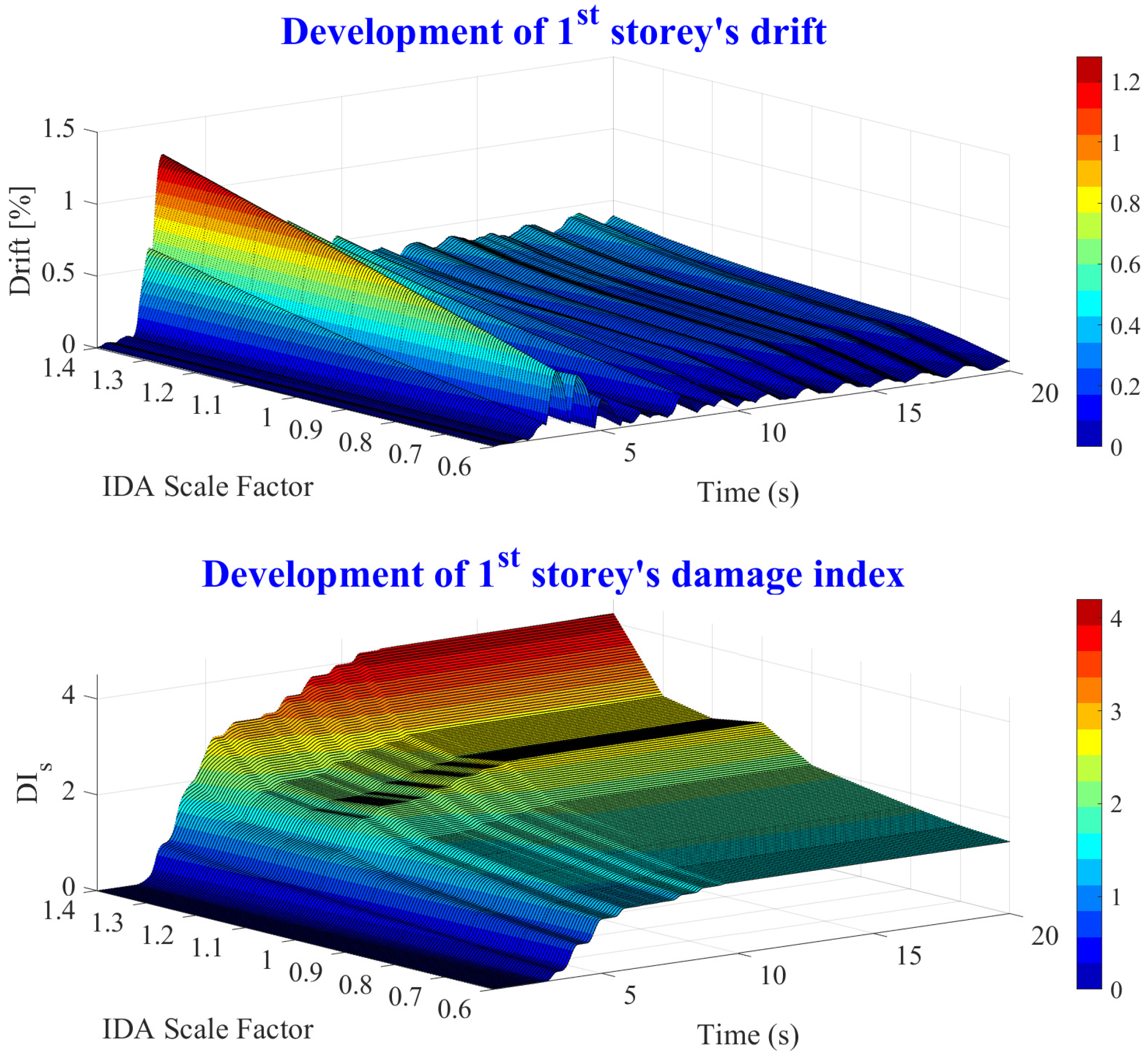
Damage occurring in base columns dominates also the global damage index value of the building, as displayed in Figure 17 and in correlation with Figure 18 where the evolution of 1st story maximum drift at each time step and the story damage index ($D{I}_s$) is represented.

The next Figure 19, Figure 20 and Figure 21, display the maximum drift and damage indices for 3rd, 6th and 9th stories. It can be seen that there exists a nonlinear correlation between maximum drift and damage indices for some of the stories. This fact indicates that for stories with such correlation a higher damage degree may be encountered. Moreover, it can be seen that drift development is mainly linear during IDA but the inherited nonlinearity shown in Figure 22 is due to maximum damage index evolution which is indeed nonlinear. At the same time, in Figure 22 it can be seen that stories with a high root mean squared error value are correlated with higher values of damage.

4. Conclusions

The main scope of this paper is to introduce a straightforward numerical routine developed in Matlab/Simulink for nonlinear dynamic analysis of reinforced concrete (RC) frames using the insights of the force analogy method coupled with an explicit integration scheme.

The accuracy of the proposed numerical algorithm is further validated through a comparison of the structural response with the results obtained by commercial software commonly used by structural engineers in structural design.

Furthermore, an energetic evaluation of the structural response was conducted. The energy balance time history was calculated using a seismic input scaled with a scale factor of $1.4$. In addition, the energy balance error was computed in each time step in order to evaluate the performance of the time integration scheme.

Moreover, in order to showcase the capabilities of the algorithm, an incremental dynamic analysis was conducted on a structural model using Vrancea 1977 seismic inputs scaled with scale factors ranging from $0.6$ to $1.4$. The structural response data was processed and a damage evaluation procedure, using damage indices, was conducted. The results reveal damage distribution among different plastic hinges and different stories of the model, together with the time evolution of story drifts. The overall building hysteresis dissipated energy and damage index are also displayed.

Compared to the well known classical approaches, the proposed routine has the following crucial advantages: Throughout the entire dynamic analysis, the initial stiffness matrix of the structure is used, and therefore no other numerical algorithm is necessary for the determination of stiffness matrix in each time step; the classical equation of motion described by a second-order differential system is reduced to a first-order differential system which is further transformed into an explicit time integration scheme that uses adaptive time steps; the technique used for implementation of hysteresis functions that describe the degrading behavior of concrete elements during cyclic loading is rather uncomplicated.

To point out some of the important results, the nonlinear dynamic procedure proposed in this paper is the first to present a detailed methodology for the implementation of polygonal hysteresis models in the FAM 3D. Moreover, validation of the results using commercial software shows very good compliance of the structural response as illustrated in Figure 9, Figure 10, Figure 11 and Figure 12. Furthermore, the performance of the time integration procedure is also evaluated using the energy balance error (Figure 13). The step error reaches a maximum value of $0.7\%$, which is situated under the limit accepted by civil engineering literature (2–5%). Another interesting result aroused form damage analysis is presented in Figure , where the percentage of dissipated hysteresis energy by plastic hinges of base columns and by the rest of the plastic hinges with respect to the total dissipated energy is illustrated. The total dissipated energy by the base columns varies linearly over IDA from $50\%$ to $30\%$. Therefore, it can be concluded that the overall amount of energy dissipated through plastic deformation is mostly influenced by the cyclic behavior of the base columns. Consequently, as the seismic scale factor is raised the plastic energy amount dissipated by beams increases.

To conclude, the authors’ main contribution is the development of a force analogy-based algorithm that can be used to conduct, in a simple manner, nonlinear dynamic analysis for RC moment-resisting 3D frame structures.

References

1. Wilson, E. Termination of the Response Spectrum Method-RSM; Civilax: Zurich, Switzerland, 2015. [Google Scholar]
2. Chiorean, C. A computer method for nonlinear inelastic analysis of 3D composite steel–concrete frame structures. Eng. Struct. 2013, 57, 125–152. [Google Scholar] [CrossRef]
3. Li, G.; Wong, K. Theory of Nonlinear Structural Analysis; Wiley: Hoboken, NJ, USA, 2014. [Google Scholar]
4. Li, G.; Li, H.N.; Zhang, Y. Displacement estimation of nonlinear structures using the force analogy method. Struct. Des. Tall Spec. Build. 2015, 24, 59–72. [Google Scholar] [CrossRef]
5. Calofir, V.; Nica, B.; Pavel, F. A Nonlinear Model to Analyze the Structures Pounding Forces During Earthquakes. Arab. J. Sci. Eng. 2020, 45, 8303–8314. [Google Scholar] [CrossRef]
6. Safaei, S.; Taslimi, A.; Tehrani, P. A study on the accuracy of force analogy method in nonlinear static analysis. Struct. Des. Tall Spec. Build. 2019, 28, e1654. [Google Scholar] [CrossRef]
7. Qu, J.T.; Shu, Y. Simplified calculation of plastic energy dissipation of MDOF system using force analogy method. In Proceedings of the 6th International Conference on Advances in Experimental Structural Engineering, Torino, Italy, 1–3 July 2015. [Google Scholar]
8. Toloue, I.; Liew, M.; Harahap, I. The Effect of Element Types on Force Analogy Method Analysis. J. Eng. Technol. Sci. 2017, 49, 785. [Google Scholar] [CrossRef] [Green Version]
9. Ningthoukhongjam, S.S.; Singh, K.D. Mass irregularity effect on seismic response of moment-resisting steel frame by nonlinear time history analysis using force analogy method. Struct. Des. Tall Spec. Build. 2021, 30, e1823. [Google Scholar] [CrossRef]
10. Nica, G.B.; Munteanu, R.I.; Calofir, V.; Iancovici, M. Modelling nonlinear behavior of 3D frames using the Force Analogy Method. Structures 2021, 35, 1162–1174. [Google Scholar] [CrossRef]
11. Iancovici, M.; Ionică, G.; Pavel, F.; Mota, F.; Nica, G.B. Nonlinear dynamic response analysis of buildings for wind loads. A new frontier in the structural wind engineering. J. Build. Eng. 2021, 47, 103708. [Google Scholar] [CrossRef]
12. Simo, J.; Taylor, R. Consistent tangent operators for rate-independent elastoplasticity. Comput. Methods Appl. Mech. Eng. 1985, 48, 101–118. [Google Scholar] [CrossRef]
13. Li, G.; Zhang, Y.; Li, H.N. Seismic Damage Analysis of Reinforced Concrete Frame Using the Force Analogy Method. J. Eng. Mech. 2013, 139, 1780–1789. [Google Scholar] [CrossRef]
14. Chao, S.H.; Loh, C.H. Inelastic response analysis of reinforced concrete structures using modified force analogy method. Earthq. Eng. Struct. Dyn. 2007, 36, 1659–1683. [Google Scholar] [CrossRef]
15. Li, G.; Zhang, F.; Zhang, Y.; Li, H.N. Nonlinear hysteretic behavior simulation of reinforced concrete shear walls using the force analogy method. Struct. Des. Tall Spec. Build. 2014, 24, 504–520. [Google Scholar] [CrossRef]
16. Reinhorn, A.; Deierlein, G.; Willford, M. Nonlinear Structural Analysis for Seismic Design—A Guide for Practicing Engineers; National Institute of Standards and Technology-U.S. Department of Commerce: Gaithersburg, MD, USA, 2010. [Google Scholar]
17. Saiidi, M.; Sozen, M. Simple and Complex Models for Nonlinear Seismic Response of Reinforced Concrete Structures; University of Illinois Engineering Experiment Station; College of Engineering, University of Illinois at Urbana-Champaign: Champaign, IL, USA, 1979. [Google Scholar]
18. Tiachacht, S.; Bouazzouni, A.; Khatir, S.; Abdel Wahab, M.; Behtani, A.; Capozucca, R. Damage assessment in structures using combination of a modified Cornwell indicator and genetic algorithm. Eng. Struct. 2018, 177, 421–430. [Google Scholar] [CrossRef]
19. Baciu, C.; Lupoae, M.; Nica, G.; Constantin, D. Experimental and Numerical Studies of the Progressive Collapse of a Reinforced Concrete-Framed Structure Using Capacity Curves. Arab. J. Sci. Eng. 2019, 44, 8805–8818. [Google Scholar] [CrossRef]
20. Naqi, A.; Roy, T.; Saito, T. Time-Dependent Damage Estimation of a High-Rise Steel Building Equipped with Buckling-Restrained Brace under a Series of Earthquakes and Winds. Appl. Sci. 2021, 11, 9253. [Google Scholar] [CrossRef]
21. Xiong, C.; Zheng, J.; Xu, L.; Cen, C.; Zheng, R.; Li, Y. Multiple-Input Convolutional Neural Network Model for Large-Scale Seismic Damage Assessment of Reinforced Concrete Frame Buildings. Appl. Sci. 2021, 11, 8258. [Google Scholar] [CrossRef]
22. Massone, L.M.; Bedecarratz, E.; Rojas, F.; Lafontaine, M. Nonlinear modeling of a damaged reinforced concrete building and design improvement behavior. J. Build. Eng. 2021, 41, 102766. [Google Scholar] [CrossRef]
23. Naderpour, H.; Mirrashid, M. A novel definition of damage states for structural elements in framed reinforced concrete buildings. J. Build. Eng. 2020, 32, 101479. [Google Scholar] [CrossRef]
24. Cheng, Y.; Dong, Y.R.; Bai, G.L.; Wang, Y.Y. IDA-based seismic fragility of high-rise frame-core tube structure subjected to multi-dimensional long-period ground motions. J. Build. Eng. 2021, 43, 102917. [Google Scholar] [CrossRef]
25. Park, Y.; Ang, A.H. Mechanistic Seismic Damage Model for Reinforced Concrete. J. Struct. Eng. 1985, 111, 722–739. [Google Scholar] [CrossRef]
26. Kunnath, S.K.; Reinhorn, A.M.; Lobo, R.F. IDARC Version 3.0: A Program for the Inelastic Damage Analysis of Reinforced Concrete Structures. Technical Report NCEER-92-0022; U.S. National Center for Earthquake Engineering Research: Milpitas, CA, USA, 1992. [Google Scholar]
27. Botez, M.; Bredean, L.; Ioani, A. Plastic Hinge vs. Distributed Plasticity in the Progressive Collapse Analysis. Acta Tech. Napoc. Civ. Eng. Archit. 2014, 57, 24–36. [Google Scholar]
28. Sezen, H. Evaluation and Testing of Existing Reinforced Concrete Building Columns. CE299 Report; University of California: Berkeley, CA, USA, 2000. [Google Scholar]
29. Ibarra, L.F.; Medina, R.A.; Krawinkler, H. Hysteretic models that incorporate strength and stiffness deterioration. Earthq. Eng. Struct. Dyn. 2005, 34, 1489–1511. [Google Scholar] [CrossRef]
30. Powell, G.H.; Chen, P.F. 3D Beam‐Column Element with Generalized Plastic Hinges. J. Eng. Mech. 1986, 112, 627–641. [Google Scholar]
31. Pavel, F.; Popa, V.; Vacareanu, R. Characteristics of Simulated and Recorded Ground Motions for Bucharest; Springer: Cham, Switzerland, 2018; pp. 17–27. [Google Scholar]
32. Christopoulos, C.; Filiatrault, A. Principle of Passive Supplemental Damping and Seismic Isolation; Eucentre: Pavia, Italy, 2006. [Google Scholar]
Figure 1. Capping bending value to capacity.
Applsci 12 01692 g001
Figure 2. The backbone curve.
Applsci 12 01692 g002
Figure 3. The general hysteresis model.
Applsci 12 01692 g003
Figure 4. Moment-plastic rotation cyclic model used in this paper.
Applsci 12 01692 g004
Figure 5. The ten story 3D framed structure.
Applsci 12 01692 g005
Figure 6. The representation of columns capacity function.
Applsci 12 01692 g006
Figure 7. FAM -based peak-oriented nonlinear dynamic model developed in Simulink.
Applsci 12 01692 g007
Figure 8. Vrancea 1977 earthquake recordings.
Applsci 12 01692 g008
Figure 9. Top story displacements time history.
Applsci 12 01692 g009
Figure 10. Base column bending moments time history.
Applsci 12 01692 g010
Figure 11. Beam bending moments time history.
Applsci 12 01692 g011
Figure 12. Beam bending moment-plastic rotation response.
Applsci 12 01692 g012
Figure 13. Energy balance time history and energy balance error time history.
Applsci 12 01692 g013
Figure 14. Development of damage index for base column plastic hinges along IDA scale factors: PH no. 1—X direction and PH no. 2—Y direction.
Applsci 12 01692 g014
Figure 15. Development of damage index for beams’ plastic hinges along IDA scale factors: PH no. 125—story, 3 beam, X direction, and PH no. 651—story, 6 beam, and Y direction.
Applsci 12 01692 g015
Figure 16. Percentage of dissipated hysteresis energy for plastic hinges of base columns and for the rest of the plastic hinges with respect to the total dissipated energy.
Applsci 12 01692 g016
Figure 17. Building maximum drift and damage index in IDA.
Applsci 12 01692 g017
Figure 18. First story’s maximum drift and damage index in IDA.
Applsci 12 01692 g018
Figure 19. Third story maximum drift and damage index in IDA.
Applsci 12 01692 g019
Figure 20. Sixth story maximum drift and damage index in IDA.
Applsci 12 01692 g020
Figure 21. Ninth story maximum drift and damage index in IDA.
Applsci 12 01692 g021
Figure 22. (Up): maximum story drift together with maximum damage indices evolution over IDA (with scale factors enclosed) for 1st, 3rd, 6th and 9th stories. (Down): RMSE after linear regression on above variables. The values above the bar plots, correspond to the minimum and maximum story’s damage index value in IDA.
Applsci 12 01692 g022