3.1. Data Preparation
During the training process of developing a mathematical model to predict a parameter value as a function of a number of other variables, most researchers tend to focus on computational aspects, while at the same time paying less attention to the database being used for the training and development of the mathematical model.
However, we firmly believe that the main emphasis should be on the database to be used, as it is the database itself that describes the behaviour of the problem being modelled. The database, whether based on experimental or analytical data, is the available knowledge which must be properly utilized during the training process of the development of the mathematical model. In this regard, the database must be reliable with a sufficient amount of data to adequately describe the problem under study.
It should be noted that the phrase “sufficient amount of data” does not necessarily imply a high amount of data, but rather datasets that cover a wide range of combinations of input parameter values, thus assisting in the model’s capability to simulate the problem. The demand for a reliable database is particularly crucial in the case of experimental databases, which are databases compiled using experimental results. In this case, significant deviations between experimental values are frequently noticed, not only between experiments conducted by different research teams and laboratories, but even between datasets derived from experiments conducted on specimens of the same synthesis, produced by the same technicians, cured under the same conditions, and tested implementing the same standards and testing instruments.
In light of the above discussion, in this study, in order to develop a comprehensive database for FOS classification under dynamic conditions, a series of models were constructed to calculate FOS using a standard geotechnical software.
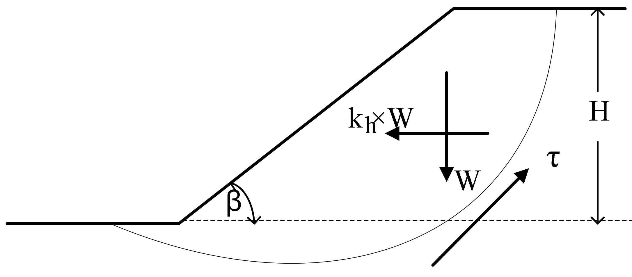
Figure 1 illustrates a generic limit equilibrium model for the simulated slope. In fact, many slope stability analysis tools use various versions of the methods of slices, such as Bishop simplified. The simplified Bishop method uses the method of slices to discretize the soil mass and determine the FOS. These methods were used in this research, the ordinary method of slices (Swedish circle method/Petterson/Fellenius), Spencer, Sarma, etc. Sarma and Spencer are called “rigorous methods” because they satisfy all three conditions of equilibrium: force equilibrium in both horizontal and vertical directions and moment equilibrium condition. Rigorous methods can provide more accurate results than non-rigorous methods. Bishop simplified or Fellenius are non-rigorous methods, satisfying only some of the equilibrium conditions and making some simplifying assumptions [
58,
59]. Some of these approaches are discussed below. Finally, slope stability analysis using Bishop simplified is a static or dynamic, analytical, or empirical method to evaluate the stability of earth and rock-fill dams, embankments, excavated slopes, and natural slopes in soil and rock. Slope stability refers to the ability of inclined soil or rock slopes to withstand or undergo movement.
The contribution of seismic loading is considered in the current slope stability analysis through the application of a horizontal force component of peak ground acceleration (PGA), that characterizes the amplitude of shaking within the sliding mass. Namely, the slope is assumed to be subjected to a force defined by
where
W is the weight of the sliding mass and
kh is a dimensionless coefficient defined by
The process was carried out in several phases to achieve a representative database. Boundary conditions, model dimensions, material properties, and seismic motion were the parameters considered in modelling. To do this, multiple homogeneous slopes with different conditions were modelled. Slopes with heights of 15, 20, 25, and 30 metres and inclinations of 20°, 25°, 30°, and 35° were produced. In terms of rigid behaviour, all of the models were placed on top of bedrock.
The failure criterion used in this method was the Mohr–Coulomb failure criterion
where
c: cohesion,
φ: friction angle,
σ: normal stress for slopes with soils with cohesion and internal friction, for a slope subjected to circular failure. The parametric values used were cohesion of 20, 30, 40, and 50 kPa and internal friction angle of 20°, 25°, 30°, 35°, and 40°. The effect of earthquake motion on slope behaviour was considered in the current analysis. For the purposes of this analysis, the soil unit weight was assumed to be 18 (kN/m
3). The amplitudes were defined as 0.1, 0.2, 0.3, and 0.4 g. On all of the slope models, thirty slices were used as slip surfaces. To achieve FOS values in this analysis, a grid and radius slip surface were used. The calculated FOS should be almost in the centre of the grid by using the grid and radius method. The FOS from the dataset was then separated manually into groups of safe slope or SS and unsafe slope or US in order to meet the objective of analysing and classifying all the slope stability cases in the dataset.
Table 2 shows the input and output parameters used in the database development.
In this study, 700 homogeneous slopes were simulated using GeoStudio which utilizes the LEM method shown in
Figure 1, along with the most critical FOS parameters. In these 700 slopes, different values of the mentioned parameters in
Table 2 were used and their FOS values were recorded. Based on a literature review conducted, the parameters presented in
Figure 1 are considered to be the most important. The best relationships between these input parameters and the output (i.e., FOS) were calculated. In this way, simple regression analysis (one to one relationship) was employed. The highest R
2 value was achieved by the PGA parameter through a polynomial trend-line (as the best trend-line among applied linear, exponential, logarithmic, and power) as follows:
A value of R2 equal to 0.305 was reported for the above equation. Besides PGA, the parameter ϕ showed the best relationship with FOS values with R2 = 0.122 through an exponential trend-line.
To determine the relative effect of each input parameter on the output parameter, a sensitivity analysis was performed. The following equation was used to perform the same analysis:
where,
rij is the strength of relation between each input and output,
is the
ith sample of input
k,
j is the number of each sample in the output set, and
m is the total number of data samples.
Table 3 shows the strengths of the relations (
rij values) between the inputs and output (FOS). The sensitivity analysis results showed that the input parameters have a great influence on the FOS. Parameter ϕ had the highest impact on FOS values followed by H, β, C, and PGA. The results obtained were in line with previous studies [
60,
61].
3.3. Decision Tree (DT)
DT is an AI technique that uses conditional judgement rules to divide predictor variables into homogeneous categories. The aim of DT specification is to find a set of decision rules for predicting an outcome from a set of input boundaries [
62]. The DT is referred to as a predictive data mining tree depending on whether the target variables are objective or subjective [
63]. Classifying the FOS of slopes from multiple input parameters is possible because modelling complex relationships between multiple input variables with an output variable is possible with a DT model as it will have both categorical and continuous variables without making any conclusions about the distribution of the provided data [
64]. Furthermore, DT models are simple to implement, and the prediction results are simple to understand. The findings of the DT model revealed the relative significance of input parameters to the output parameter [
65].
A root node, internal nodes, and leaf nodes make up a DT structure. All of the input variables are stored in the root node. A decision function is connected with an internal node, which may have two or three branches. The output of a given input vector is represented by a leaf node [
42].
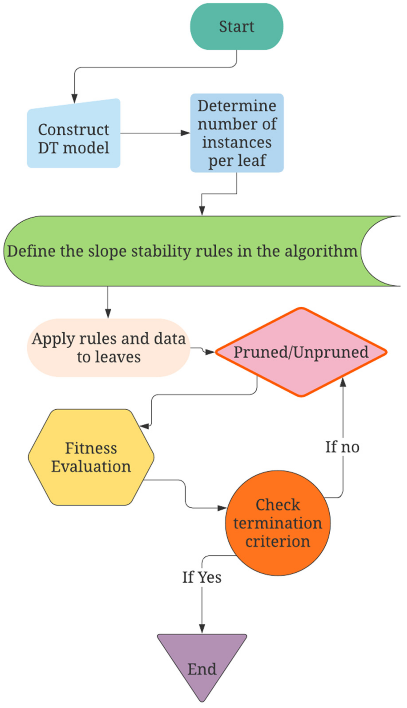
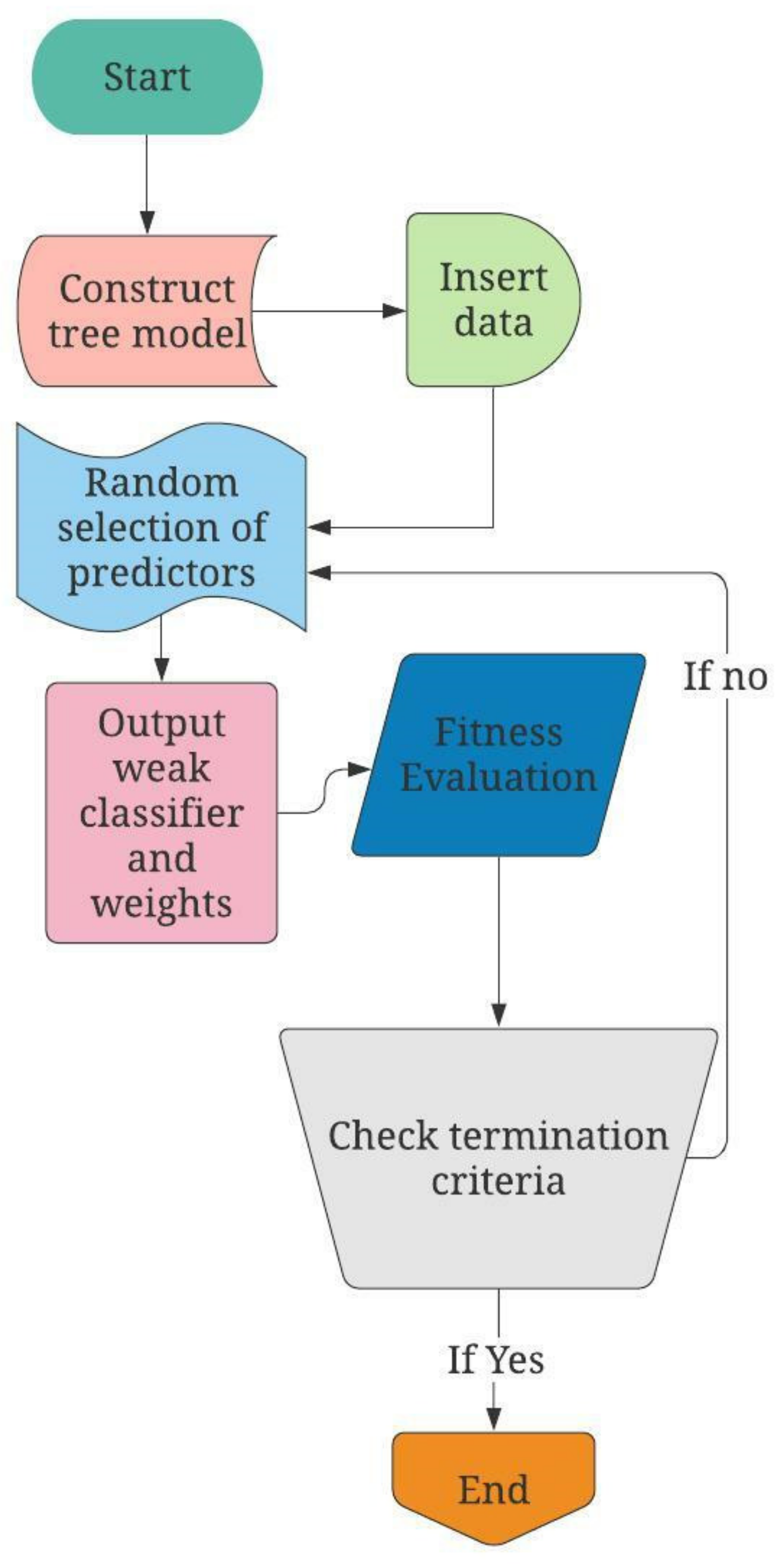
Figure 3 shows the flowchart of procedures conducted for the modelling of a DT model. The procedure of modelling a DT model is governed by two steps: tree building and pruning.
In the first step, the root node of the DT is defined by determining the input vector with the maximum gain ratio. The dataset is then divided into sub-nodes depending on the root values. For discrete input variables, each potential value is represented by a sub-node of the tree [
66]. The gain ratio is then calculated for each of the sub-nodes separately in the second process, and the process is replicated until all of the instances in a node are classified the same way. Leaf nodes are such nodes, and their names are the class values. Since the tree produced during the design process will have a large number of branches, it will be vulnerable to over-fitting [
67], it must be pruned in order to improve the prediction performance for new data. Tree pruning can be divided into two categories: pre-pruning and post-pruning. In the case of pre-pruning, the tree’s development will be halted before another criterion is true; in the case of post-pruning, the whole tree will be grown first, and then the finished subtrees will be replaced by leaves based on the tree’s flaw relation before and after eliminating sub-trees. More explanations regarding DT models can be found in [
54].
3.6. Performance Indicators
To measure the performance of the results obtained from the DT, RF, and AdaBoost models against each other and the expected results obtained from the GeoStudio software, a few performance indicators were used. These performance indicators were accuracy, precision, recall, F1-score, and ROC curve. All the models were subjected to the performance indicators to observe their effectiveness. Accuracy is the ratio of the number of correctly classified predictions divided by the total number of projections. It ranges from 0 to 1. Equation (7) shows the calculation of accuracy where True Positive and True Negative are correct predictions made by the model.
Precision is the measurement of positive class predictions that actually belong to the positive class, which in turn calculates the accuracy of the minority class. This calculation is expressed in Equation (8) where the False Positive represents the false positive prediction made by the model.
Recall is a statistic index that measures how many accurate positive assumptions were made out of all possible positive expectations. Unlike precision, which only considers true positive predictions out of all predictions, considering the positive predictions that were wrong. This calculation is expressed in Equation (9) where the False Negative represents the false negative prediction made by the model.
F1-score is a method for combining precision and recall into a single measure that encompasses both. Neither precision nor recall can provide the full picture on their own. We may have excellent precision but poor recall, or vice versa, poor precision but good recall. With the F1-score, all issues with a single score can be expressed (Equation (10)).
ROC curve or receiver operating characteristic curve is a graph of the false positive rate (x-axis) vs. the precision (y-axis) with a variety of candidate thresholds ranging from 0.0 to 1.0. The false positive rate is determined by dividing the total number of false positives by the total number of false positives and true negatives. With all the performance indicators mentioned above, the area under the ROC curve could be obtained for each model. This value will represent the effectiveness of each model.


 ,
, 


