1. Introduction
With the increase in mining depth, coal mine disasters are increasing, such as coal and gas outburst [
1,
2,
3], rock burst [
4,
5,
6], and large deformation of surrounding rock [
7,
8,
9,
10,
11,
12], which bring severe challenges to the safe and efficient mining of deep coal resources. The in-situ stress is one of the most critical factors, as it is not only the fundamental force leading to the disasters, but also has great impacts on gas pressure, rock burst degree, rock mass deformation, and strength characteristics. Therefore, in order to achieve the effective control of coal mine disasters, accurate and reliable in-situ stress data must be obtained through field measurement.
Hydraulic fracturing and overcoring are the two most widely used in-situ stress measurement methods at present [
13,
14,
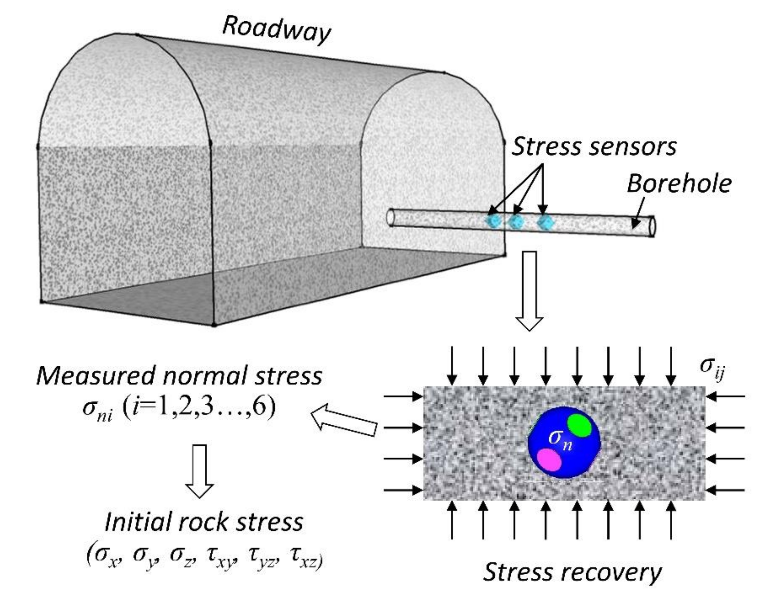
15]. Both of them are suitable for rock masses of substantial hardness and integrity. However, due to the influence of the sedimentary environment and tectonic movements, the deep rock masses of coal mines are usually weak and/or broken, which often leads to measurement failure. For this reason, a novel in-situ stress measurement technique, specialized for deep fractured rock masses, was put forward as the rheological stress recovery (RSR) method [
16,
17,
18]. It is based on the strong rheological characteristics of fractured rock masses under high stress, and carried out by embedding the stress sensors into the drilling holes filled with grout. Due to the strong rheology of rock masses, the stress near the sensors gradually recovers. Meanwhile, the measured stress of the sensors increases and eventually stabilizes. The initial rock stress was finally evaluated via the recovery data obtained from the stress sensors (
Figure 1).
According to the measuring principle of the RSR method, since the stress state of a point contains six stress components, the sensor needs to obtain six normal stresses in different directions to calculate the rock stress. However, in the field of geotechnical engineering, the commonly used pressure sensors are unidirectional and can only obtain one normal stress, such as the various pressure boxes used for measuring earth pressure, lining pressure, and pulling pressure of the anchor rod and cable [
19,
20,
21]. In order to achieve multidirectional normal stress measurements, a three-direction vibrating wire pressure sensor was developed [
22]. It resembles a cube, and contains three orthogonal pressure sensing units with a maximum range of 30 MPa (
Figure 2). Based on the three-direction pressure sensor, the RSR method has been successfully applied to obtain in-situ stress measurements in Pingdingshan No.1 and No.11 coal mines [
17,
22,
23]. At the same time, several problems have been found in the field. Firstly, the sensor is bulky and inconvenient to install. Secondly, it is difficult to determine the three-dimensional attitude of the sensor in the borehole. Thirdly, the proximity of the two sensors to each other can easily cause stress field disturbance, which is difficult to evaluate.
In recent years, due to the outstanding advantages of anti-electromagnetic interference, electrical insulation, and intrinsic safety, fiber optic sensing technology has been widely applied in coal mines. Many coal mines in China have established a sound optical fiber communication system, laying the foundation for the monitoring and early warning of deep coal mine disasters and the construction of smart mines. Meanwhile, in the field of sensor development, which includes such instruments as the fiber Bragg grating (FBG) sensor [
24,
25,
26], distributed fiber optic sensors and fiber optic gas sensors have been developed and widely applied due to their high measurement accuracy and stability. Based on the testing principle of the RSR method and fiber optic sensing technology, this paper developed a new FBG stress sensor to solve the problems existing in the current three-direction pressure sensor, and provides support for the application of the RSR method for use on fractured rock masses in deep coal mines.
3. Calibration Equipment and Tests
3.1. Calibration Equipment
Due to the novel structure of the developed FBG sensor, it is inconvenient to calibrate it with traditional calibration test equipment. Therefore, a simple calibration device specifically for the FBG sensor was designed and manufactured (
Figure 13). The device consists of support frame, guide, and load components. The support frame includes four adjustable bases, a bearing plate, and a sensor base. The guide component includes four guide bars that are fixed onto the bearing plate. The load component includes a loading plate, a loading bar, and some weights. The weights are placed onto the loading plate and the forces are transferred to the sensing unit via the loading bar.
3.2. Calibration Test
The calibration test aimed to check and verify the measurement performance of the sensor. According to the applicable fields of the FBG sensor, the national standards of China (JJG860-2015), and the common calibration methods for fiber optic sensors described in the literature, the calibration test program for the developed FBG sensor was formulated.
(1) Sensor preloading: Temperature will have an influence on the sensor. Based on previous experience in field stress testing, we decided to set 20 °C as the calibration temperature. Firstly, put the sensor in the laboratory for more than 2 hours at room temperature, 20 °C, to eliminate the effect of temperature change. Then, place the sensor in the calibration device for preloading. Each sensing unit preload is divided into three levels: 80, 160, and 240 kg, respectively, which correspond to the loading pressures 10, 20, and 30 MPa, respectively. For each preloading level, the loading stability time is set as 5 min. After loading, unload the sensing unit to a zero pressure state, and adjust the sensor position for the next preloading of the sensing unit. The purpose of preloading is to make close contact between the sensor parts to ensure that the sensing units will be of strong working condition and that the wavelength output will be more stable. At the same time, check whether the calibration device and related test instruments are working properly, and whether the test data output are accurate.
(2) Sensor cyclic loading: After preloading, the cyclic loading tests are carried out for each sensing unit. The specific steps are as follows:
① Place the sensor into the sensor base of the calibration device, adjust the senor unit and dowel bar to ensure they are coaxial, and record the initial output wavelength of the sensing unit. ② Put weights onto the loading plate of the calibration device with successive loading steps of 20 kg. After stabilizing for 2 mins, record the wavelength of the FBG demodulator under the corresponding load. Unload the weights when loading reaches 240 kg and the unloading path is consistent with the loading process. ③ Repeat step ②three times so that each sensing unit has three loading and unloading cycles. ④ Repeat steps ①–③ until all sensing units are calibrated. ⑤ Remove the sensor from the calibration device and end the calibration test.
The process of the calibration test is shown in
Figure 14. As FBG is a temperature-sensitive material, temperature changes will affect the accuracy of calibration data. Therefore, during the test, the temperature change should be kept within ±5 °C, and the current temperature should be recorded every 30 mins. If the temperature change exceeds ±5 °C, the test data will be invalid and will need to be re-calibrated.
In order to check the test performance of the sensor under long-term working conditions, the stability test was carried out. The stability test can obtain the long-term stability of the sensor by applying long-term stability load to the sensing units and observing the change in the output wavelength of the sensing units with time. The test load was set to the full range, i.e., 30 MPa. The loading time was 24 days and the data recording time interval was 24 h.
4. Results and Discussion
The calibration curves of the sensor are shown in
Figure 15. According to the calibration test data and the standard National Metrological Verification Regulation JJG860-2015 Pressure Sensor (Static) of China, the sensing characteristic index and measurement error index of the sensor were investigated. The sensing characteristic indexes include the maximum working range, the output value of the full range, and the sensitivity, etc., whereas the measurement error indexes include the linearity index, the zero drift index, the hysteresis index, and the repeatability index, etc. The specific definitions of each index are as follows.
The output value of the full range is defined as:
where
λf is the output value of the full range, n is the total number of calibration loading and unloading cycles, and
λimax (
λimin) is the wavelength output value at the upper (lower) limit of the measurement when the sensing unit is under the
ith cycle.
Zero drift refers to the fluctuation of the output value of the calibrated sensor in the absence of external load, which is defined as:
where
d is zero drift,
di is the
ith zero output record, and
d1 is the first zero output record.
The linear fitting formula of the sensing unit can be obtained by fitting the calibration test curve with the least square method:
where
y is the output wavelength,
x represents the external load,
k is the slope of the fitting curve, and
λB is the initial wavelength of the sensor. Then, the linearity is defined as:
where
is the average value of the output wavelength at the
ith calibration point and
yi is the corresponding value of the calibration point on the fitted line.
Repeatability refers to the repetition degree of the output data of the calibrated sensor. It is used to investigate the reliability and stability of the sensor, and is defined as:
where
K is the standard deviation over the entire range, and is defined as:
where
KLi is the standard deviation for
ith calibration point during loading,
KUi is the standard deviation for
ith calibration point during unloading,
n is the number of calibration cycles,
i is the sequence number of the calibration point,
j is the sequence number of the calibration cycles,
yLij is the output wavelength for the
jth cycle at the
ith calibration point during loading,
is the average wavelength at the
ith calibration point during loading,
yUij is the output wavelength for the
jth cycle at the
ith calibration point during unloading,
is the average wavelength at the
ith calibration point during unloading, and m is the number of calibration points.
Hysteresis refers to the difference between the output wavelength of the sensor at the calibration point, which mainly reflects the accuracy and assembly performance of the sensor. It is defined as:
Sensitivity refers to the change in the FBG wavelength per MPa, and is defined as:
where
Pmax is the maximum working range.
According to the above definitions and calculation formulae, the characteristic indexes of the sensor are calculated. As can be seen in
Table 2, the maximum working range of the sensor calibration is 30 MPa, the output wavelength of the full range is 2688 to 2900 pm, and the sensitivity ranges from 89.600 to 96.656 pm/MPa. According to Equation (2), there is a linear relationship between wavelength drift and fiber strain. Considering the elastic-optic coefficient,
Pe, is 0.216 for common fiber materials, the strain of full-range fiber grating can be calculated as 2238.273 to 2390.323.
Table 3 reveals that the zero drift index of the sensor ranges from 0.035 to 1.158%, the linearity index ranges from 0.392 to 1.225%, the repeatability index ranges from 0.139 to 0.833%, the hysteresis index ranges from 0.281 to 1.166%, and the error index is within the range of 1.5%.
The stability test results for 1
#, 3
#, and 5
# pressure sensing units are shown in
Figure 16. It indicates that there is a creep phenomenon in the sensing unit under the long-term load, and the creep drift changes rapidly during the first few days, which gradually slows down in the later period, and finally stabilizes. According to the calibration coefficient and wavelength variation, the long-term measurement errors of the 1
#, 3
#, and 5
# sensing units were calculated as 1.51, 1.50, and 1.45%, respectively.
Fiber wavelength division multiplexing (WDM) technology was adopted for the sensor to ensure that only one channel of the optical fiber demodulation instrument was occupied for a single sensor. That is, each sensing unit took up a different wavelength range, and then the optical fibers for each sensor were welded into the coupler box. As a result, only one optical fiber connector of the sensor was outputted. In order to achieve the use of the sensor in the coal mine, an intrinsically safe optical fiber demodulator was developed. The wavelength demodulator range is 1,525 to 1,565 nm. Based on this, the wavelength range of each sensing unit was designed to be 5 nm (-1 to 4 nm), that is, the wavelength change of each sensing unit under tension was no more than 1 nm, and the wavelength change under pressure was no more than 4 nm.
According to the calibration test data, the initial wavelength of sensing units 1
# to 6
# are: 1,531.80; 1,537.05; 1,542.44; 1,547.35; 1,552.51; 1,557.43 nm, respectively. It was calculated that the initial wavelength interval of sensing units 1
# to 6
# is 4.91–5.25 nm, basically consistent with the wavelength design range of the sensing unit. According to
Table 2, the wavelength varies from 2,688 to 2,900 pm when the sensing unit is subjected to 30 MPa, which is approximately 67.2 to 72.5% of the designed wavelength range (4 nm), indicating that the design range of the sensor has sufficient redundancy.
In general, the performance of the sensor developed in this paper reaches the level of accuracy index 2.0, which meets the test requirements for engineering applications. However, due to the limitations of processing conditions and cost, the precision and assembly level of the sensor parts still require improvement, and the accuracy level could also be further improved. In addition, the sensor test used in this paper is limited to the routine calibration and stability tests, and the calibration results cannot be directly applied to the practical engineering environment. In order to apply the sensor in field, more numerical and/or physical simulation studies are needed to master the test performance of the sensor under different working conditions.


