Numerical Study of Coupled Fluid and Solid Wave Propagation Related to the Cladding Failure of a Nuclear Fuel Rod

Abstract

Fuel rod cladding failure in a nuclear reactor produces different phenomena related to vibrations and fluid–structure interaction. The most significant aspect of those phenomena is the creation of a pressure wave at the failure position and its propagation in the coolant fluid flowing around the fuel rod. An accurate understanding of the propagation of the pressure wave around the fuel rod can help us design a method to detect a failure, determine its position, and estimate some of its characteristics with a single and simple sensor, such as a pressure sensor or a piezoelectric acoustic sensor, that can be mounted relatively far from the failure. Such a method can be useful for the monitoring of nuclear fuel rods, where instrumentation possibilities are restricted (because of neutron flux, radiation, high temperature, and available space) as well as for any kind of application involving annular ducts and limited instrumentation possibilities. The current paper is related to the specific application of nuclear fuel rod monitoring. It deals with preliminary numerical simulations that are necessary to know the evolution of a fluid pressure profile along the system containing the rod. They are carried out by finite element methods, using the EUROPLEXUS code. They provide the necessary information about the propagation of pressure waves around the rod to design measurement and signal processing methods as well as properly interpret experimental results from tests in industrial reactors, research reactors, or experimental mock-ups. They also provide some information that could not be experimentally obtained because of the constraints in a nuclear environment. Despite the specific application we show in this article, similar calculation methods, theoretical observations, and results interpretations can be easily adapted to the other mentioned applications.

1. Introduction

In most pressurized water nuclear reactors (PWR), fuel material consists of small pellets that are inserted in thin metallic tubes. Such a metallic tube is called a cladding, and the element consisting of the cladding filled with fuel pellets is referred to as a fuel rod. In industrial plants, thousands of fuel rods are gathered in the reactor core and are surrounded by axially flowing water, which acts as a coolant fluid. The cladding is supposed to physically separate the fuel material from the surrounding water. However, because of combined effects of corrosion, mechanical fretting, high temperatures, and chemical load of fission product, cladding failures can occur during reactor operation. Under some conditions, the failure can produce a pressure wave that propagates in the surrounding water. Such a phenomenon is more likely to occur during a Reactivity-Initiated Accident, as explained in [1,2].

The detection, localization, and characterization of cladding failures are of interest for studies about fuel behavior in research reactors as well as for optimizing the operation of industrial power plants. However, this phenomenon occurs inside the reactor core, where there are high temperatures, radioactivity, and little available space. Therefore, instrumentation possibilities for failure detection are limited. In such a situation, acoustic and vibration methods are interesting. Thanks to wave propagation phenomena, it is possible to measure waves generated by a source in a limited access area with distant sensors. Concerning a cladding failure in a reactor core, waves propagating in either the structure or the coolant fluid can be used. Indeed, both types of wave can be related to the cladding failure: right after the cladding failure, a fast increase in pressure of the surrounding fluid occurs, because of a thermal reaction between ejected fuel particles and surrounding fluid and, in case of a waterlogged rod, a release of high-pressure steam that was contained inside the rod. The pressure surge generates waves that propagate in the fluid and therefore can be measured by pressure sensors. An increase in the fluid pressure also induces additional stresses in the structure because of fluid–structure interaction. The induced stresses propagate as elastic waves through the structure (the rod and the outer structure) and can be measured by acoustic emission (AE) sensors mounted on the outer structure (The so-called acoustic emission methods consist in studying high-frequency elastic waves generated by damage mechanisms. Therefore, in the current article, acoustic emission sensors are considered as vibration sensors, as vibration refers to elastic waves in the structure).

Another advantage of using fluid pressure waves and elastic waves is the possibility to measure them with simple and robust sensors such as piezoresistive and piezoelectric sensors. Those technologies enable producers to design pressure sensors and AE sensors that can withstand radioactivity and relatively high temperature. They are not resistant enough to be placed in the middle of the core, but they can be mounted close to the rod ends. However, the acoustic signals that would be measured during tests in a reactor would be affected by noise, by unknown events, and by propagation effects (dispersion, reflection and fluid–structure interaction). Thus, in order to properly interpret these signals, identify unknown events, and potentially improve measurements techniques, we need more information about wave propagation and fluid–structure interaction than what measurements can provide. We especially lack information about velocities of the different types of waves, signal distortion due to the propagation through a geometrically complex system, and transmission between fluid and solid media. To improve the understanding of these phenomena, we decided to obtain missing information by calculation methods. We focus here on the case of the experimental devices used in research reactors for the study of a single rod rather than the industrial systems case containing several rods. Some analytical methods may be able to approximate pressure and stress evolution in a very simplified model of the device, such as the methods developed for studies on water hammer ([3,4]). Nevertheless, because of the complex geometries of devices used in research reactors, specific and accurate calculations were necessary to get results that could be compared with experimental data from real tests in a reactor. Thus, a numerical model of a typical experimental device was built to run finite element computations.

A numerical approach enables a relatively accurate model of the structure (in terms of geometry and material composition). However, modeling the failure phenomenon and its direct effects requires a lot of information that are not available in the literature. Moreover, characteristics of such a phenomenon are complex and deeply depend on experimental conditions and the initial state of the rod (such as its internal composition, burn-up, initial leakage, cladding oxidation, etc.), as explained in [1,2]. Therefore, it is impossible to precisely estimate general failure characteristics and build a numerical model of the phenomenon that would be representative of every possible failure. Hence, the objective of the numerical approach presented in this paper is to obtain information about wave propagation and the associated fluid–structure interaction, without an exhaustive and realistic simulation of the failure phenomenon itself. Although propagation phenomena depend quantitatively on the system properties, the global phenomenological interpretation that is presented here is valid for every system consisting in a metal structure and a liquid-filled annular channel.

The current paper deals with preliminary calculations that are necessary to better understand the evolution of pressure profile in the fluid and stress profile in the structure along the part of the device containing the tested fuel rod. Only the results related to pressure in the fluid are presented, because the interpretation of structural wave signals depends too much on the sensor being used, whose response highly affects the measured signal. While the response of commercial pressure sensors can be assumed to be flat up to 25% of their resonant frequency (usually given by the producer) and the output of such sensors can reliably be considered as the actual pressure (which is a simple scalar value), the interpretation of AE sensors’ signals leads to some issues. Firstly, most of the AE sensors are intended to be used at their resonant frequency and have consequently a non-flat response. Secondly, the actual physical value measured by the sensor (displacement, velocity, acceleration) and the directivity is seldom known. Estimating the response of AE sensors is a recurrent problem that has been studied several times (for instance, [5,6,7]). The results depend on the model of the sensor, and there is currently no simple solution to accurately estimate an AE sensor response. As a consequence, the interpretation of the raw physical values provided by the numerical simulation is suited for signals measured by any model of fluid pressure sensors, but it might be unsuited for AE sensors signals.

The first part of the paper consists of the description of a typical experimental test device (materials, geometry, flow parameters). The second part describes the numerical model and the methodology used for the computation. The results are introduced, analyzed, and discussed in the third part.

As a result of non-disclosure obligation, physical values cannot be explicitly shown. Thus, length and pressure values are given in arbitrary units, which are defined in the following section. The arbitrary unit of length, referred to as A.U.L., is defined as the length of the main section of the device (Figure 1). Its order of magnitude is one meter. The arbitrary unit of pressure, referred as A.U.P., is defined as the maximum value measured by the pressure sensors. Its order of magnitude is 100 bar.

2. Description of the System

The studied system is based on the typical geometry of experimental devices used in French research reactors for the study of a single rod’s behavior (for instance, the REPNa devices in the CABRI reactor [8], GRIFFONOS and ISABELLE devices in the OSIRIS reactor [9], the forthcoming ADELINE device in the RJH [10]). Such a device contains a fluid channel where the tested rod sample is placed. The device is inserted in the reactor (usually a pool reactor) that generates a neutron flux representative of the one met by a rod in an industrial reactor. The channel containing the tested rod is connected to an independent water loop that recreates typical thermohydraulic conditions of industrial pressurized water reactors (water at 280 °C and 155 bar, flowing at 3.4 $\mathrm{m}·{\mathrm{s}}^{-1}$).

The typical characteristics of such a device are as follows:

• An overall length of several meters;
• A central section of about one meter, containing a fuel rod sample of about 60 cm;
• A structure mostly made of stainless steel and, in the central section, Zircaloy (because of its neutron-transparency property);
• Various instrumentation downstream and upstream from the central section.

In the current study, only the central section and its inlet and outlet sections are considered. Figure 1 shows a simplified drawing of this central section. Typically, this part can be described as an annular structure with several coaxial layers. From the outside to the inside, these layers are an external tube, an annular gap filled with gas, a second tube made of Zircaloy (called the “channel tube” in Figure 1), an annular water channel, and the tested fuel rod. The gaseous gap is intended to mechanically and acoustically separate the inner channel from outside events. In this paper, we focus on what happens inside the test device only and neglect the effects of the external layer. Thanks to the gaseous gap, these are realistic simplifications (it was verified in a real device that the sensors are almost insensitive to outside events). Thus, we consider only the part of the device including the channel tube, the water channel, and the fuel rod. Only that part is presented in Figure 1, which shows a simplified drawing of the studied part of the test device. In the following paragraphs, we refer to the channel tube as the “outer structure”. From a longitudinal point of view, the section upstream from the rod is called the “inlet section”, the section downstream is called the “outlet section”, and the section containing the rod is called the “main section”. The main section is separated from the inlet and outlet sections by short transition sections. In these transition sections, the channel cross-section is reduced to enable a mechanical connection between the outer structure and the rod and extensions assembly. There, the channel cross-section is not annular but consists of several holes. For the sake of understanding, an example of such a transition cross-section is shown in Figure 2.

Several measurement points are considered in the system. Two of them, referred to as P1 and P2, are located in the inlet and outlet sections and can be considered as realistic measurement points, as it is actually possible to place sensors at equivalent positions in a real device (see Figure 1). Therefore, they show the actual possibilities that can be expected from pressure measurements in a real reactor. The other points, defined in Section 4, are located in the central section, or very close to it. They are used to get information for the understanding of the studied phenomena, but they are not related to available sensor positions in the real device.

As it is the case in real devices, geometrical singularities of the channel lie between main section and the inlet and outlet sections, because of the mechanical supports of the rod and its extensions. The geometry is not symmetrical between the inlet side and the outlet side, which results in different wave paths between the source and the P1 and P2 sensors, as it is also the case in real devices.

Real devices are actually vertically inserted in the core, and water flows from the bottom to the top. In Figure 1, the inlet is on the right and the outlet is on the left.

3. Methodology for the Numerical Simulation and Results Analysis

A 3D model of the central section of the device was built. This model includes a partial description of the outer structure, of the test rod with its extensions, and of the fluid domain between them. It also includes a compressed gas bubble in a cavity inside the rod, expanding in the surrounding fluid through a small hole in the cladding. Here, we consider still water, because the actual flow speed (3.4 $\mathrm{m}·{\mathrm{s}}^{-1}$) is very low compared to the characteristic pressure wave speed (about 1100 $\mathrm{m}·{\mathrm{s}}^{-1}$ in water in the test conditions). However, simulating initially flowing water is straightforward and might be attempted in further study if needed. Numerical simulations are computed with EUROPLEXUS software (currently abbreviated EPX [11]). It is a simulation software using finite elements and finite volume methods for fluid–structure interaction problems. An explicit time integration algorithm makes the software especially suited to fast transient phenomena, such as a fuel rod cladding failure. In the present study, computation in the structure and in the fluid domain are respectively performed with Lagrangian and Arbitrary Lagrange Euler representations, along with gas–water interface tracking in the fluid to produce sharp pressure loading (see [12]). The simulation duration is 2.5 ms. It is enough to observe the propagation of the relevant waves in both structure and fluid (assuming that the lowest wave speed is about 1100 $\mathrm{m}·{\mathrm{s}}^{-1}$ as mentioned above, which is a reasonable approximation for the wave speed in water at 280 °C and confined in an elastic tube). The calculation time step is adaptive, but the results are stored every ${10}^{-6}$ s. The full computation for approximately 400,000 elements requires about 230,000 s CPU on a local workstation with limited parallel resources (see [13] for parallel framework in EPX).

3.1. Fluid Model

Both fluid components are modeled with the stiffened gas equation of state (for details about the definition of this equation from the Grüneisen Equation of State, refer to [14]; for details about its implementation in EPX, refer to [15]):

$$p=(\gamma -1)\rho (e-q)-\gamma P_{\infty }$$

(1)

where p is the fluid pressure, $\gamma$ is an empirical constant (equal to heat capacity ratio for a perfect gas), q is the formation energy (we can simply take $q=0$ because no phase change is considered here, see [16]), $\rho$ is the fluid density, e is the internal energy, and $P_{\infty }$ is a constant associated to the molecular attraction needed to represent liquids such as water. Thus, the term $(\gamma -1)\rho$ is related, in this case, to the molecular repulsion effects, and $\gamma P_{\infty }$ represents fluid cohesion.

Damping in the fluid due to shock waves after the initial expansion of the compressed bubble is approximated by Neumann–Richtmyer artificial viscosity ([17]).

The average axial, radial, and circumferential dimensions of a fluid element in the main section are respectively about 3 mm, $0.5$ mm, and 1 mm. Around geometrical singularities, the mesh is refined.

3.2. Geometry and Structure

Dimensions of the model are based on the characteristics mentioned in Section 2 and shown in Figure 1. Although real devices often contain some small asymmetrical parts, they have been neglected here so that the structure of the model is purely axisymmetrical, except at the transition sections, where the through holes are symmetrical with respect to a longitudinal plane. Neglected asymmetrical parts are located on the outer surface of the structure. Therefore, they do not influence the behavior of the inner fluid. Thus, in order to reduce computation cost, and assuming that the studied phenomena are symmetrical, only a half portion of the real system was modeled (from 0° to 180°). Therefore, while the real system has a cylindrical shape, the model has a semi-cylindrical shape. Symmetry conditions are applied on the cutting plane (x-y plane, with x being the longitudinal axis and y being a transversal axis), by imposing the displacements normal to the plane to be zero.

In real devices, the different parts of the outer structure are welded. In the model, welded joints are modeled as simple planar interfaces with rigid connections. Connections between the rod and its extensions at both ends are rigid. Mechanical connections between the rod extension and the outer structure in the model are representative of real ones. The lower rod extension (on the right of Figure 1) is rigidly connected to the outer structure at the inlet transition, and the upper rod extension (on the left) is pinned to the outer structure at the outlet transition.

The fuel model is simplified in a homogeneous solid volume instead of several stacked pellets. The cladding is modeled with shell elements (four nodes shell elements based on [18] and referred to as “$Q4GS$” in EPX, see [19]); the fuel cylinder and all the other structural parts are modeled with cubic elements (“$CUBE$” elements in EPX). The average axial, radial, and circumferential dimensions of an element of the outer structure around the main section are respectively about $2.3$ mm, $1.5$ mm, and 2 mm. Around geometrical singularities, the mesh is finer (axial, radial, and circumferential dimensions of the finest elements located in the inlet transition are about 2 mm, 0.5 mm, and 1 mm). This size is a compromise between (1) the aim of accurately simulating fast variations of pressure and velocity around geometrical singularities and (2) computation cost. The calculation time step and, hence, computation cost depends directly on the mesh size in the structure. Then, for the sake of accuracy, the fluid mesh is adjusted to match the structural mesh. Moreover, as the fluid is inviscid, it is not necessary to refine fluid mesh in the radial direction near the boundary. Figure 3 shows views of the mesh around the inlet and the outlet transitions, where there are the most significant geometrical singularities.

Every structural part is modeled with its respective material (zircaloy, stainless steel, fuel material). Small pieces such as wires, screws, or sensors are neglected.

3.3. Material Properties

The material properties used for the simulation are given in

Table 1. Structure materials properties.

Material	Density ($\mathbf{kg}·{\mathbf{m}}^{-3}$)	Young’s Modulus (GPa)	Poisson’s Ratio
Steel	7830	176	0.3
Zircaloy-4	6560	78	0.4
Fuel	10,500	80	0.37

and

Table 2. Fluid materials properties.

Material	Density ($\mathbf{kg}·{\mathbf{m}}^{-3}$)	${\mathit{P}}_{\mathit{\infty }}$ (Pa)	$\mathit{\gamma }$
Water (liquid)	764	4500	1.896
Water (gas)	1	0	1.4

. They are approximated properties of the corresponding materials at 280 °C and 155 bar, which are the average pressure and temperature in the test device and in industrial PWR. No damping is applied to the structure. Elastic deformation only is considered. The effects of temperature changes on structural material properties are disregarded, because the characteristic time associated to temperature variations is much longer than the time associated to the propagation of the waves along the whole system.

In a fluid represented by the stiffened gas equation of state, with a density ${\rho }_f$, the sound speed is given by ([16]):

$$c_{w0}=\sqrt{\frac{\gamma }{{\rho }_f}(P+P_{\infty })}.$$

(2)

Then, the sound speed in liquid water at 155 bar, 280 °C, is $c_{w0}=1075\mathrm{m}·{\mathrm{s}}^{-1}$. This value refers to the speed of sound in an infinite volume of fluid; it does not take any structure into account. The sound speed in the gaseous phase has no practical importance here. Since no phase change is simulated, the volume of the gaseous phase remains very small compared to the liquid volume and stays close to its initial location during the whole simulated time.

3.4. Simulation of the Cladding Failure Effects

The objective of this study is not to achieve an accurate simulation of the failure itself but to obtain information about wave propagation phenomena in the specific system corresponding to the test device. Hence, cladding failure is modeled in a rather simplified way. Neither material distortion nor fuel–coolant thermal interaction are simulated. We only reproduce the over-pressure resulting from these phenomena and propagating through the system. To reproduce this over-pressure, a cavity was created inside the rod. That cavity is initially filled with pressurized gas at a higher pressure than the surrounding fluid pressure. That gas can represent pressurized fission gas, internal steam in case of a water-logged rod, or the pressure surge induced by fuel–coolant interaction. The contact area between the gas in the cavity and the surrounding fluid is obtained with an aperture in the cladding. At the beginning of the simulation, pressurized gas is released in the surrounding fluid, creating a pressure wave that propagates along the system, in both directions (downstream and upstream). The cavity inside the rod is axisymmetrical, but the aperture in the cladding stretches only over a reduced part of the cladding circumference and is not axisymmetrical. Thus, it results in an asymmetrical source and enables the observation of 3 dimensional effects, which is necessary to estimate the validity of the plane wave assumption.

In the axial direction, the cavity and the cladding aperture in the model have the same length. The results that are presented in this article come from a simulation computed with an arbitrary failure position, which is set at $135.3\times {10}^{-3}$ A.U.L. from the lower end of the rod. In real experiments, the position of the failure depends on the initial state of the rod and the experimental conditions.

The influence of the failure length in the model is discussed in Section 4.2.

4. Results and Discussion

4.1. Theoretical Remarks

In order to properly interpret the numerical results, a short introductory theoretical study is useful. Its objective is to have approximated values for the velocities of the different kinds of waves that can be observed in the system. On that purpose, previous works on “water hammer” phenomena are used.

In the studied problem, pressure waves in fluid and elastic waves in the structure have to be considered as well as their mutual interaction. The excitation source we focus on is the local over-pressure induced by the failure. In the numerical model, there is no other source. The local over-pressure mainly propagates as pressure waves in the fluid. In addition to that, because pressurized fluid exerts loads on the structure walls, elastic waves are also created and propagate in the structure. With common materials (such as steel, zircaloy, and water), elastic waves in the structure travel faster than pressure waves in fluid, so the elastic wavefront goes ahead of the pressure wavefront. Then, elastic waves can partially radiate back to the fluid. As a consequence, small pressure fluctuations, induced by structural waves radiation, precede the main pressure wavefront. On the pressure history calculated or measured at a given point, small fluctuations appear therefore before the main peak corresponding to the pressure wavefront. Those fluctuations are called “precursor waves”. We refer to the main pressure wavefront as the “primary wave” ([20]).

For both types of waves, plane wave assumption can be considered for long wavelengths (i.e., low frequencies). This assumption simplifies not only analytical equations but also qualitative interpretation of numerical or experimental results, especially concerning elastic waves. In an elongated structure, such as a tube, longitudinal and shear waves combine together, depending on boundary conditions, and create guided waves. Different stress profiles over the cross-section can be associated with guided waves. Each possible stress profile is identified as a propagation mode. Guided waves are usually dispersive (i.e., propagation speed depends on the frequency), and each mode has a specific dispersion curve. With plane wave assumption, guided wave phenomena can be neglected, and only the fundamental wave types (longitudinal and transverse waves, which have constant velocities) can be considered. Moreover, according to [3], longitudinal waves effects are predominant in the low-frequency range. Therefore, “precursor waves” in the low-frequency range are assumed to be mainly related to axial waves (Structure axial waves induce fluid pressure fluctuations because of the Poisson effect, which creates transversal motion associated with tension–compression stresses. Without the Poisson effect, pressure fluctuations could be induced by friction effects only and therefore would be very low and almost invisible). Considering that pressure wave resulting from the failure is similar to the one resulting from water hammer, we can use some results of the four equations model of water hammer introduced in [21] and extended in [4] (among many others). This model is not presented here; we only introduce some of its results concerning wave speeds.

Let us consider a pipe with an internal radius R and a wall thickness e. The pipe is made of a material with density ${\rho }_s$, Young’s modulus E, and Poisson’s coefficient $\nu$ and is filled with a fluid of density ${\rho }_f$. Based on the four equation water hammer model, primary wave (i.e., fluid pressure wave) speed is given by ([4]):

$$c_f=\sqrt{\frac{1}{2}({\beta }^2-\sqrt{{\beta }^4-4c_{w1}^2{c}_L^2})},$$

(3)

where $\beta$ is a constant introduced for the sake of readability:

$${\beta }^2=(1+2{\nu }^2\frac{{\rho }_f}{{\rho }_s}\frac{R}{e}\frac{1}{1+\frac{e}{2R}})c_{w1}^2+c_L^2,$$

(4)

where $c_{w1}$ is the sound speed in a fluid contained in an elastic pipe and the sound speed in an incompressible fluid contained in an elastic pipe $c_{w0b}$ ($c_{w1}$, defined in Equation (5), does not include the effects of pipe vibrations on the wave speed in the inner fluid, contrary to $c_f$, as defined in Equation (3), and only takes in account the pipe wall stretching due to the pressure load). In [22], its value is deduced from the sound speed in the unrestrained fluid ($c_{w0}$, which is defined in Equation (2)). $c_{w1}$ is defined as:

$$c_{w1}=\frac{c_{w0}{c}_{w0b}}{\sqrt{c_{w0}^2+c_{w0b}^2}},$$

(5)

with $c_{w0b}=\sqrt{\frac{Ee}{2R{\rho }_f}}$ .

$c_L$ is the longitudinal wave velocity in a bar:

$$c_L=\sqrt{E/{\rho }_s}.$$

(6)

Finally, with water properties given in Table 2, $R=7$ A.U.L. and $e=7.5$ A.U.L. (which are the dimensions of the channel tube), we obtain: $c_f=1062\mathrm{m}·{\mathrm{s}}^{-1}$.

The theoretical velocity of precursor waves is defined by:

$$c_s=\sqrt{\frac{1}{2}({\beta }^2+\sqrt{{\beta }^4-4c_{w1}^2{c}_L^2})}.$$

(7)

With the material properties given in Table 1 and dimensions mentioned above, it yields $c_s=3160\mathrm{m}·{\mathrm{s}}^{-1}$. $c_s$ is close to the typical longitudinal wave velocity in Zircaloy-4 ($c_{Zr4}=\sqrt{\frac{E_{Zr4}}{{\rho }_{Zr4}}}=\sqrt{\frac{78\times {10}^9}{6560}}=3448\mathrm{m}·{\mathrm{s}}^{-1}$). It is actually the typical longitudinal wave velocity with light modification due to the Poisson effect and the fluid–structure interaction.

In that preliminary study, only a simple pipe representing the outer tube was considered, rather than two coaxial tubes, which would better represent the complete system. However, the objective was simply to get approximated velocities to guide the interpretation of numerical and experimental results. Thus, it was considered that the necessary work to accurately adapt the four-equation water-hammer model to the studied case was not relevant in the frame of this study.

4.2. Numerical Results: Effects of the Failure Length

Before analyzing numerical results in details, preliminary observations regarding the length of the simulated failures are introduced.

It is assumed that the failure length influences the resulting pressure variation in the fluid, in both simulations and real situations. When numerical results are compared to experimental results from a failure test in a real reactor, the failure length in the model should be actually compared to the size of the reaction area where the over-pressure is produced in the real test and to the pressure profile in this area. However, the estimation of those characteristics is not simple. The most direct information that can be provided by tests in a real reactor are pressure histories in the inlet and the outlet section, which are given by sensors P1 and P2 (assuming that measurements closer to the failure are not possible). Depending on the possibilities in other kinds of measurements, some characteristics can be estimated afterwards. The exact starting point of the cladding failure can be determined by visual examination of the rod after the experiment. The initial size of the reaction area, the kinetic of the failure, and the fuel ejection might be deduced from temperature and energy deposit, depending on the measurement possibilities. However, such estimations require extensive works that are far beyond the scope of the present study. Moreover, as shown in [1,2], these characteristics significantly depend on rod properties and are difficult to predict.

Given the large variability in the lengths of real failures, and since the accurate estimation of the actual over-pressure area may not be possible, the comparison between simulation results and future experimental results will likely require several simulation iterations with various failure lengths. To predict the effects of the failure length on the pressure that could be measured in the device, simulations with three different failure lengths (3 mm, 15 mm, and 30 mm) were performed. Fluid pressure histories in the outlet and inlet sections (at the “realistic” measurement points) obtained with the different failure lengths are presented in Figure 4. For the sake of readability, pressure variations around the initial pressure value (155 bar in absolute value) are presented rather than absolute pressure values. Unless otherwise stated, it is the case for all pressure values in the present article.

The effects of the differences in the failure length are clearly shown in Figure 4. The longer the failure is, the wider the first pressure peak on the signal. In the next part of the article, results obtained with a 30 mm are used. The choice is arbitrary, but, despite the noticeable difference in the signals, the analysis methodology and the physical interpretation is the same for any failure length.

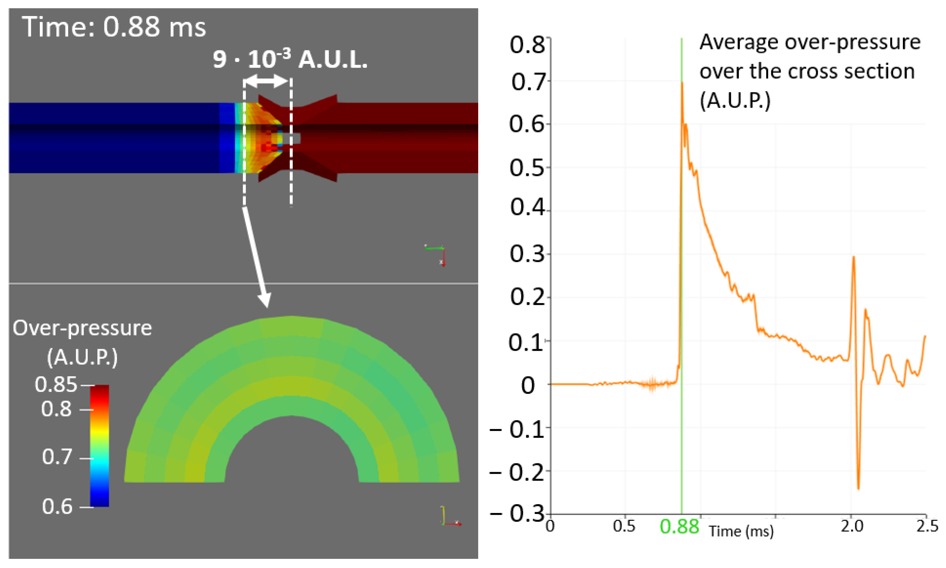
4.3. Numerical Results: Pressure History at Different Positions

The signals used in this part are the average pressure over the cross-section at defined axial positions. As the pressure field shows in Figure 5, Figure 6 and Figure 7, pressure waves can reasonably be considered as plane waves. It allows the use of the cross-section average pressure instead of the value at a point with specific angular and radial coordinates.

Figure 8 shows the pressure history at six different axial positions in the main channel. Figure 9 shows these positions.

Each signal in Figure 8 can be divided in four parts:

• An empty part before signal arrival;
• Low-amplitude waves (hardly visible on Figure 8; see Figure 10);
• Main wave front followed by slow pressure decrease;
• First reflection followed by additional resonance.

The main wave front is assumed to be the primary wave (propagation of the pressure wave in water), and low-amplitude waves appearing before the main wavefront are assumed to be precursor waves. Precursor waves are hardly visible in Figure 8, but we can clearly see them with a magnification such as the example in Figure 10. They are also slightly noticeable on some frames in Figure 5 and Figure 6.

To confirm that interpretation, we estimate the velocities of the observed low-amplitude waves and main wavefront to compare them with the theoretical values of precursor and primary waves. Velocities are estimated by the time difference of arrival (TDOA) between the different signals. TDOA is estimated for each couple of signals (such as the example in Figure 11); then, the average value is computed. We obtain the following average values (with a 95% confidence interval):

• For the early low-amplitude waves (assumed precursor waves): $3550\pm 132\mathrm{m}·{\mathrm{s}}^{-1}$;
• For the main wave front (assumed primary wave): $1052\pm 9\mathrm{m}·{\mathrm{s}}^{-1}$.

These values are quite close to the values given by the simplified theoretical model (Section 4.1) for precursor and primary waves. Therefore, our interpretation can be confirmed.

The channel in the main section has a quasi-constant cross-section (there is only a small and gradual increase of 40% of the cross-section, upstream from the rod, due to a change in upper extension diameter). Therefore, in that area, the distortion of propagating waves is very low, so two pressure signals extracted at two different positions in that section look very similar. In Figure 8, if we look at the first peak only, all the signals look quite similar and differ almost exclusively by time shifts (after the first peak, more significant differences arise because of reflections on channel ends). One may especially notice that the amplitude of that first peak is nearly constant over the six positions. However, at the transitions between the main section and the inlet or outlet sections, there are strong and steep cross-section reductions. These reductions are necessary to make a mechanical connection between the rod extensions and the outer structure and, thus, to hold the rod, but they disrupt wave propagation, especially fluid pressure waves. Waves propagating from a source around the rod (such as a cladding failure) to P1 or P2 sensors cross either the inlet or the outlet transition. Therefore, signals that are measured by these sensors are affected by the perturbation due to these geometrical changes. Pressure histories at several positions around the outlet transition (the positions are shown in Figure 12) are shown in Figure 13. The first peak amplitude on downstream positions is clearly lower than on upstream positions. That difference is due to the strong reflection at the downstream edge of the transition. Pressure histories at the two downstream positions clearly exhibit a second pressure peak, which is related to the reflected pressure wave. It shows that as the wave first travels through the system, a large part of its energy stays in the main section and does not enter the outlet sections. This phenomenon is also noticeable in Figure 6.

4.4. Numerical Results: Source Localization Methods

To introduce failure localization methods, we assume we know neither the failure position nor its occurrence time. In such a case, several simple methods to find the position are available with our current results:

• Based on the time difference of arrival (TDOA) of the primary wave between two positions in the main section, one downstream and one upstream from the failure. Source position is estimated with the following expression:

  $$x_s=\frac{(x_i+x_j-c_f\Delta t)}{2}$$

  (8)

  with $x_i$ and $x_j$ representing the axial positions of the two points from which pressure histories are extracted, $\Delta t$ representing the TDOA between the two points, and $c_f$ representing the primary wave speed.
• Based on the TDOA of the primary wave between P1 and P2. Source position is given by the previous expression.
• Based on the time delay between precursor waves and the primary wave at a single point (either a point in the main section, or P1, or P2). Assuming that precursor waves and the primary wave are created at the same point and at the same time, the source position is deduced from the following:

  $$d=(t_f-t_s)\frac{c_f{c}_s}{c_s-c_f}$$

  (9)

  with d representing the distance between the source and the point from which the pressure signal is extracted, $c_f$ representing the primary wave speed, $c_s$ representing the precursor wave speed, $t_f$ representing the arrival time of the primary wave, and $t_s$ representing the arrival of the precursor waves.

These methods require either an assumption about wave velocities (we can use, for instance, the analytical Formulas (3) and (7) or the average values deduced from our numerical results), or an additional point to estimate them by TDOA. In the latter case, the first two methods would require two points on one side of the failure and a third point on the other side. The third method would require two points on the same side of the failure.

Here, we applied these methods with assumed velocities (both with analytical ones and with the ones previously deduced from the numerical results). Hence, the first two methods require two sensors; they are referred to as “multi-sensor methods”, and the third requires a single sensor only and therefore is called a “single-sensor method”. Results obtained with the different methods are presented below. All positions are relative to the lower end of the rod.

Multi-sensor localization with points in the main section:

TDOA is estimated between each of the points shown in Figure 8, which are downstream from the failure, and the point C0, which is upstream from the failure (the failure is quite close from the main section lower end, so only one upstream point is considered), as shown in Figure 9. Then, the source position is estimated with Equation (8). The average value is eventually calculated. Results are shown in

Table 3. Multi-sensor localization with points in the main section—results (actual source position: $135.3\times {10}^{-3}$ A.U.L.).

Points	Points’ Positions (${10}^{-3}$ A.U.L.)	TDOA ($\mathsf{\mu }$s)	Assumed Wave Speed (m · s−1)	Resulting Source Position (${10}^{-3}$ A.U.L.)
C0; C1	44.0; 222.9	$-1.5\pm 2$	1062	$134.2\pm 2.8$
			$1052\pm 9$	$134.2\pm 2.8$
C0; C2	44.0; 312.7	$87\pm 2$	1062	$136.0\pm 2.8$
			$1052\pm 9$	$136.4\pm 3.5$
C0; C3	44.0; 402.4	$182\pm 2$	1062	$134.5\pm 2.8$
			$1052\pm 9$	$135.4\pm 3.9$
C0; C4	44.0; 592.1	$275\pm 2$	1062	$134.1\pm 2.8$
			$1052\pm 9$	$135.4\pm 4.3$
C0; C5	44.0; 581.8	$369\pm 2$	1062	$133.4\pm 2.8$
			$1052\pm 9$	$135.1\pm 4.8$
Average			1062	$134.5\pm 2.8$
			$1052\pm 9$	$135.3\pm 3.6$

.

Multi-sensor localization with P1 and P2:

TDOA is estimated between P1 and P2, and the source position is deduced with Equation (8). The results are given in

Table 4. Multi-sensor localization with P1 and P2—results (actual source position: $135.3\times {10}^{-3}$ A.U.L.).

Points	Points’ Positions (${10}^{-3}$ A.U.L.)	TDOA ($\mathsf{\mu }$s)	Assumed Wave Speed (m · s−1)	Resulting Source Position (${10}^{-3}$ A.U.L.)
P1; P2	−324.8; 1490.0	$919.6\pm 4$	1062	$134.7\pm 3.9$
			$1052\pm 9$	$138.8\pm 7.7$

.

Single-sensor localization

Localization results with the pressure history at different points in the main section are given in

Table 5. Single-sensor localization with points in the main section—results (actual source position: $135.3\times {10}^{-3}$ A.U.L.).

Point	Point’s Position (${10}^{-3}$ A.U.L.)	Time Delay Precursor- Primary Waves ($\mathsf{\mu }$s)	Assumed Wave Speed (m · s−1)		Resulting Source Position (${10}^{-3}$ A.U.L.)
			$c_f$	$c_s$
C2	312.6	$87\pm 3$	1062	3160	$150.5\pm 4.4$
			$1052\pm 9$	$3550\pm 132$	$161.1\pm 8.3$
C3	402.4	$182\pm 3$	1062	3160	$143.4\pm 4.4$
			$1052\pm 9$	$3550\pm 132$	$160.3\pm 10.9$
C4	492.1	$275\pm 3$	1062	3160	$133.3\pm 4.4$
			$1052\pm 9$	$3550\pm 132$	$156.8\pm 13.5$
C5	581.8	$369\pm 3$	1062	3160	$122.5\pm 4.4$
			$1052\pm 9$	$3550\pm 132$	$152.5\pm 16.1$
Aver.			1062	3160	$137.4\pm 4.4$
			$1052\pm 9$	$3550\pm 132$	$157.7\pm 12.2$

. C1 is not used here because it is close to the failure, and therefore, the time delay between the precursor and primary waves is too short to yield an accurate result.

Localization results with the pressure history at P1 or P2 are given in

Table 6. Single-sensor localization with P1 or P2—results (actual source position: $135.3\times {10}^{-3}$ A.U.L.).

Point	Point’s Position (${10}^{-3}$ A.U.L.)	Time Delay Precursor- Primary Waves ($\mathsf{\mu }$s)	Assumed Wave Speed (m · s−1)		Resulting Source Position (${10}^{-3}$ A.U.L.)
			$c_f$	$c_s$
P1	607.3	$325\pm 3$	1062	3160	$152.2\pm 7.3$
			$1052\pm 9$	$3550\pm 132$	$121.0\pm 19.3$
P2	1874	$4000\pm 3$	1062	3160	$6.2\pm 7.3$
			$1052\pm 9$	$3550\pm 132$	$103.2\pm 45.5$

.

Figure 14 shows the localization results with the different methods, except the inconsistent value of the single-sensor localization with P2 and numerically estimated velocities (last row of Table 6). Here, using analytical velocities provides smaller uncertainties than using values deduced from TDOA on numerical results. Actually, there is no uncertainty on the analytical wave speeds because we could use the exact same material properties for the determination of analytical velocities and for the numerical computation. However, in an experimental context, there are uncertainties regarding the material properties and consequently on the analytical estimation of the wave speed. Depending on these uncertainties, using analytical velocities may not be more reliable than estimating them by measurements with additional sensors.

5. Conclusions

Numerical simulations were computed with the EUROPLEXUS software to improve the understanding of fluid–structure interaction phenomena related to fuel cladding failure in a nuclear reactor and, thus, to design a failure localization method based on pressure signals analysis.

The simulations allow the confirmation of several phenomenological assumptions. The observation of the spatial evolution of the pressure profile proves that the plane wave assumption is valid. It also shows that a geometrical singularity in the channel leads to reflections of the pressure waves and, consequently, transmission loss between the two sides of the singularity. Moreover, the time evolution of the pressure at different positions of the system exhibits two kinds of waves, referred as precursor and primary waves, according to the terminology used in water-hammer studies.

The simulations also bring quantitative information about the velocities of precursor and primary waves, which can be estimated from the simulated signals. They were compared to analytically determined values and proved to be consistent with them. This quantitative information can be of interest for the analysis of experimental results, since the measurements that are necessary to estimate waves velocities may not be possible in a real reactor.

From a practical perspective, the simulations show that precursor and primary waves appearing in pressure signals can be used to detect and locate the failure. Thus, detections and localizations can be achieved with a single sensor, using the time difference of arrival (TDOA) between the two kinds of waves, although using the TDOA between the primary waves of two different sensors’ signals provides more accurate results. Moreover, precursor waves have a small amplitude compared to the primary waves, and although they are detectable in noiseless simulated signals, they might be hidden by noise in experimental signals.

Despite the useful information provided by the simulations, some limits of the current numerical model have been identified:

• Simulated phenomena are simplified: only the transient over-pressure due to the failure is simulated. Material failure or distortion and fuel pieces ejection are not simulated, even though they might happen in the real case. This simplification is related to the reproduction of the excitation phenomenon, but it is independent from the results related to propagation phenomena;
• Coolant fluid vaporization is not reproduced, although it affects the wave propagation. Nevertheless, the characteristic time associated to phase changes is much longer than the time associated to the propagation of precursor and primary waves along the whole system, which is the main phenomenon considered in this article. The earliest effect of a phase change that may affect the first failure-induced waves is the apparition of small bubbles at the beginning of the boiling stage. This would result in a slight decrease in pressure wave velocity but would not significantly change the aspect of the wavefront. Moreover, coolant fluid vaporization does not occur at every failure.

For the simulations presented in this article, a uniform temperature of 280 °C and a single-phase coolant fluid were considered. A sensitivity analysis should be carried out to accurately assess effects of the temperature field and of possible changes in pressure wave velocities caused by steam bubbles in the coolant fluid.

Furthermore, the numerical model still needs to be validated by comparisons with experimental results. To this aim, an experimental mockup was designed and is currently being used at the Cadarache center of the French Commission for Atomic and alternative energies (CEA) [23]. In this mockup, the failure of fake fuel rods is reproduced, and the resulting fluid pressure waves and vibrations are recorded at several positions of the system. Thus, the fluid pressure profile evolution along the system will be compared to the numerical results to validate the model presented in the current article. Measurements related to elastic waves in the structure, carried out with AE sensors, strain gauges, and accelerometers, will be compared to the numerical results in order to estimate the bias induced by the response of those sensors.

After this validation, the numerical model can be used according to the presented methodology for the interpretation of experimental results from tests in a real reactor. In such a case, it will be necessary to adjust some parameters, such as the failure length and position, to make the simulation representative of the specific test being analyzed.