A Two-Step Surface Reconstruction Method Using Signed Marching Cubes

Abstract

In this paper, we explore a new approach, a two-step surface reconstruction method to extract the target isosurface from a given implicit function efficiently. Our main contribution is that we improve the surface reconstruction process by accelerating the speed of evaluation using signed marching cubes. The basic strategy is to filter the invalid voxels that do not intersect with the target isosurface in a low-cost manner, and to evaluate the valid voxels that intersect with the target isosurface accurately. The improved signed marching cubes method consists of a rough evaluation step and an exact evaluation step. The coarse evaluation step evaluates the points of all voxels using the fast multipole method with a lower order. After the rough evaluation step, the voxels that intersect with the target isosurface are screened out. Then, the exact evaluation step evaluates the points of filtered voxels using the fast multipole method with a higher order. The experimental results show that, compared with the traditional marching cubes method, the improved reconstruction method reduces the amounts of calculation for invalid voxels that do not intersect with the target isosurfaces, which is useful to improve the efficiency of surface reconstruction.

1. Introduction

Reconstructing a surface from a series of geological sampling points is a well-studied problem in geological modeling, computer graphics, and reverse engineering, etc. In geological modeling, the implicit modeling method [1,2,3,4] interpolates the geological sampling points to obtain an implicit function representing the best fitting geological surface. To visualize the interpolated implicit function, the implicit surface reconstruction method [5,6,7] should be used to extract the target isosurface of the interpolated implicit function. What is proposed in this paper is the tracing of a surface (two-manifold) in 3D, but similar concepts have been investigated in other cases (e.g., polynomial systems [8,9]).

There are many implicit surfaces reconstruction methods used to extract isosurfaces, including the marching cubes (MC) methods [10,11,12,13,14,15,16], the marching tetrahedra (MT) methods [17,18], and the Delaunay triangulation methods [19,20,21]. The marching cubes method is widely used for its efficiency and robustness. Based on the given implicit function, the basic idea of the marching cubes method is to triangulate the sampling points by evaluating the corresponding function values. The evaluation points are sampled regularly by a specified voxel size in the modeling space. Then, the target isosurface is extracted by triangulating the sampling points to approximate the target isosurface based on the eight vertices of each cube and a predefined lookup table. For the quality of the triangular mesh, Dietrich et al. [22] presented an edge transformation method for improving the mesh quality of the marching cubes to reduce degenerate triangles. Raman et al. [23] extended the lookup table, which differentiates scalar values equal to the isovalue from scalar values greater than the isovalue, in order to improve the quality of reconstructed mesh. For the correctness of the mesh topology, there are several methods [24] presented to resolve the ambiguity of the isosurface for any cube configuration.

The motivation of this paper is to reconstruct an implicit surface from a given implicit function efficiently by improving the evaluation process of the classical marching cubes method. The performance of implicit surface reconstruction involves the space complexity and the time complexity [25]. An important limitation of the classical marching cubes method is that it takes too much time to evaluate the points of invalid voxels that do not intersect with the target isosurface. To deal with this problem, a common approach is to track the valid voxels that intersect with the target isosurface using the surface following strategy [26]. However, the surface following method depends on the initial seed voxels to reconstruct the target isosurface. In addition, the method may fail to recover the complete isosurface if the initial seed seeds are not sufficient. Therefore, in this work, to accelerate the evaluation process, we try to develop a two-step reconstruction method, including a coarse evaluation step and a refine evaluation process.

The key idea of the two-step reconstruction method is based on the fact that, for the radial basis functions (RBF) method [27,28,29], the target zero isosurface can be evaluated by the sign of the implicit function using different expansion orders according to different evaluation precisions. The fast multipole method (FMM) [30,31,32,33,34] is used to accelerate the evaluation of RBF-based implicit functions. A higher expansion order of the fast multipole method obtains a more accurate function value, but it consumes more time than a lower expansion order. Cuno et al. [11] proposed a marching cubes hierarchical adaptive algorithm for fast polygonization of variational implicit surfaces. As mentioned earlier, the surface following method improves the traditional marching cubes method by tracking the adjacent target voxels to recover the isosurface via some given seed voxels that intersect with the target isosurface. Therefore, similar to the surface following method [26], a natural strategy is to approximately determine the voxels that intersect with the target isosurface with a lower expansion order.

In this paper, we present a two-step surface reconstruction method to extract the implicit surface for the RBF method without specified seed voxels efficiently. Our main contribution is that we improve the surface reconstruction process by accelerating the speed of evaluation using signed marching cubes. The method no longer tracks the potential voxels that intersect with the target isosurface directly based on the given seed voxels. It filters most of invalid voxels that do not intersect with the target isosurface with a low cost. In addition, different from the traditional surface following method, it ensures that the reconstructed isosurface is complete. It is worth noting that geological data were used for experiments, but other types of data (e.g., medical or mechanical engineering CT scans) are a legitimate input as well.

2. Method

2.1. Radial Basis Functions Interpolation

The RBF interpolation method is widely used in surface modeling as it is well suited to scattered data interpolation problems. In this paper, taking the RBF interpolation method as an example, we analyzed the two-step reconstruction method. The RBF interpolant $s\left(\mathit{x}\right)$ is a function of the following form [35]

$$s\left(\mathit{x}\right)={\displaystyle \sum }_{j=1}^N{\omega }_i\Phi \left(\mathit{x},{\mathit{x}}_j\right)+p\left(\mathit{x}\right)$$

(1)

where $\left\{{\mathit{x}}_1,{\mathit{x}}_2,\dots ,{\mathit{x}}_N\right\}$ is a set of different interpolation points, and ${\omega }_i$ is the weight coefficient to be determined. $\Phi \left(\mathit{x},{\mathit{x}}_j\right)$ is a radial basis kernel function. $p\left(\mathit{x}\right)$ is the polynomial part. For example, the first-degree polynomial is a function of the following form

$$p\left(\mathit{x}\right)=c_1+c_{2}x+c_{3}y+c_{4}z$$

(2)

where $x,y,z$ are the coordinate components of the evaluation point $\mathit{x}$ and $c_1,c_2,c_3,c_4$ are the weight coefficients to be determined. In general, the polynomial part should satisfy the side conditions of the form

$${\displaystyle \sum }_{i=1}^N{\omega }_i={\displaystyle \sum }_{i=1}^N{\omega }_i{x}_i={\displaystyle \sum }_{i=1}^N{\omega }_i{y}_i={\displaystyle \sum }_{i=1}^N{\omega }_i{z}_i=0$$

(3)

where $x_i,y_i,z_i$ are the coordinate components of point ${\mathit{x}}_i$.

To interpolate the implicit function $s\left(\mathit{x}\right)$, the geological sampling data should be converted into the interpolation constraints of the form

$$s\left({\mathit{x}}_i\right)=f_i,\hspace{1em}i=1,2,\dots N$$

(4)

where $f_i$ is the function value at the interpolation point ${\mathit{x}}_i$.

The interpolation constraints and the side conditions are combined to form a linear system of the following form

$$\left[\begin{array}{cccccccc}{\Phi }_{11}& {\Phi }_{12}& \cdots & {\Phi }_{1N}& 1& x_1& y_1& z_1\\ {\Phi }_{21}& {\Phi }_{22}& \cdots & {\Phi }_{2N}& 1& x_2& y_2& z_2\\ ⋮& ⋮& \ddots & ⋮& ⋮& ⋮& ⋮& ⋮\\ {\Phi }_{N1}& \Phi & \cdots & {\Phi }_{NN}& 1& x_N& y_N& z_N\\ 1& 1& \cdots & 1& 0& 0& 0& 0\\ x_1& x_2& \cdots & x_N& 0& 0& 0& 0\\ y_1& y_2& \cdots & y_N& 0& 0& 0& 0\\ z_1& z_2& \cdots & z_N& 0& 0& 0& 0\end{array}\right]\left[\begin{array}{c}{\omega }_1\\ {\omega }_2\\ ⋮\\ {\omega }_N\\ c_1\\ c_2\\ c_3\\ c_4\end{array}\right]=\left[\begin{array}{c}{f}_1\\ f_2\\ ⋮\\ f_N\\ 0\\ 0\\ 0\\ 0\end{array}\right]$$

(5)

where

$${\Phi }_{ij}=\Phi \left({\mathit{x}}_i,{\mathit{x}}_j\right)$$

(6)

The unknown coefficients of $s\left(\mathit{x}\right)$ can be calculated by solving the above linear system.

2.2. Signed Fast Multipole Method

To recover the interpolated surface of an implicit function, it is necessary to sample the geometry space and evaluate the function values of the sampled points. The efficiency of the surface reconstruction mainly depends on the process of evaluation. The direct evaluation of a radial basis function with $N$ constraint points requires $O\left(N\right)$ operations. To accelerate the speed of evaluation, the fast multipole method can be utilized to approximate the function values of radial basis functions within a given precision.

Given a set of target points (evaluation points) $\left\{\mathit{x}\right\}$ and source points (interpolation points) $\left\{\mathit{y}\right\}$, the basic idea of the fast multipole method is to represent the RBF kernel using a finite series [35].

$$\Phi \left(\mathit{x},\mathit{y}\right)={\displaystyle \sum }_{n=1}^p{\varphi }_n\left(\mathit{x}\right){\psi }_n\left(\mathit{y}\right)+R_p\left(\mathit{x},\mathit{y}\right)$$

(7)

where $p$ is the expansion order of the series ${\varphi }_n$ and ${\psi }_n$. $R_p\left(\mathit{x},\mathit{y}\right)$ is a residual that satisfies $R_p\left(\mathit{x},\mathit{y}\right)\to 0$ for ${\parallel \mathit{x}-\mathit{y}\parallel }_2\to \infty$ and/or $p\to \infty$.

Then, the summation of RBF kernels can be evaluated at the evaluation points $\left\{\mathit{x}\right\}$ via the following formula

$$f\left(\mathit{x}\right)=s_p\left(\mathit{x}\right)+{\epsilon }_p$$

(8)

where

$$s_p\left(\mathit{x}\right)={\displaystyle \sum }_{j=1}^N{\omega }_j\Phi \left(\mathit{x},{\mathit{y}}_j\right)={\displaystyle \sum }_{n=1}^p{\varphi }_n\left(\mathit{x}\right)\left[{\displaystyle \sum }_{j=1}^N{\omega }_j{\psi }_n\left({\mathit{y}}_j\right)\right]={\displaystyle \sum }_{n=1}^p{\Psi }_n\left(\mathit{y}\right){\varphi }_n\left(\mathit{x}\right)$$

(9)

The moments ${\Psi }_n\left(\mathit{y}\right)$ can be pre-computed firstly. The evaluation error ${\epsilon }_p$ satisfies

$${\epsilon }_p={\displaystyle \sum }_{j=1}^N{\omega }_j{R}_p\left(\mathit{x},\mathit{y}\right)>0$$

(10)

Note that the evaluation points should be far away from the source points to ensure the expansion order is small enough. Therefore, the multilevel fast multipole method [36] is developed to construct the finite series using several fast multipole method operations, including P2M, M2M, M2L, L2L, L2P, and P2P. In this paper, the kernel independent fast multipole method (black-box fast multipole method [37]), is utilized to evaluate the function values of the radial basis functions efficiently.

In general, the higher the expansion order $p$ of a series is, the smaller the approximate residual will be. That is, a higher expansion order corresponds to a higher accuracy of the evaluated kernel function value and a smaller evaluation error ${\epsilon }_p$. However, sometimes it is not necessary to spend too much time to compute the accurate function value, but only to determine the sign of the function value. In this case, we can utilize a lower expansion order to determine the sign of the function value. Therefore, how to determine the positive and negative sign of the function value is a key problem. The relationship between the expansion order $p$ and the evaluation error ${\epsilon }_p$ can be defined as

$$f\left(\mathit{x}\right)=s_p\left(\mathit{x}\right)+{\epsilon }_p=\left\{\begin{array}{l}>0, if s_p\left(\mathit{x}\right)>0 and s_p\left(\mathit{x}\right)-{\epsilon }_p>0\\ <0, if s_p\left(\mathit{x}\right)<0 and s_p\left(\mathit{x}\right)+{\epsilon }_p<0\end{array}\right.$$

(11)

Considering that the absolute function values of the points that are far away from the target isosurface are greater than the evaluation error ${\epsilon }_p$, it is possible to evaluate the sign of the function values using a lower expansion order at these points. In other words, we can select a lower expansion order in the process of evaluation to filter the non-boundary voxels that are far away from the target isosurface.

To distinguish different kinds of voxels, the evaluation voxels are divided into two kinds: the non-boundary voxels (including the exterior voxels and the interior voxels) and the boundary voxels. The seed points near the target isosurface are used to determine the seed voxels, as shown in Figure 1. The absolute function values of the points on the non-boundary voxels are greater than the evaluation error ${\epsilon }_p$.

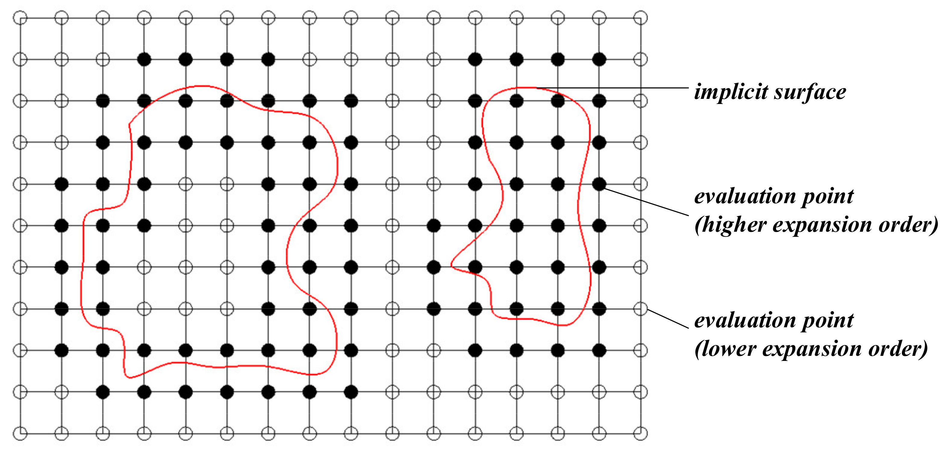
2.3. Two-Step Surface Reconstruction Method

The ideal of the marching cubes method is to evaluate all partitioned voxels in a specified 3D space to extract the target isosurface for an implicit function, as shown in Figure 2a. The method can recover a complete model. However, it should traverse and calculate all voxels in the 3D space, which consumes a lot of time to filter the non-boundary voxels that do not intersect with the target isosurface.

To improve the reconstruction efficiency, the voxel growing (VG) method is developed to deal with the problem that the marching cube method takes a lot of time to calculate non-boundary voxels. The method tracks the boundary voxels by searching the adjacent voxels based on some initial seed voxels, as shown in Figure 2b. However, it also leads to a new problem, in that it depends on reliable seed voxels to recover a complete model. In general, at least one seed voxel should be determined to reconstruct each separate isosurface in the geometry space.

Based on the above analysis, we present the signed marching cubes method (SMC) to accelerate the speed of surface reconstruction combined with the signed fast multipole method. It is useful to avoid the invalid evaluation of non-boundary voxels that do not intersect with the target isosurface.

To improve the evaluation efficiency, the expansion order should be optimized to minimize the calculation and complexity on the premise of satisfying the reconstruction accuracy. The basic idea is to determine the optimized expansion order according to the evaluated function value and its corresponding evaluation error. For the exterior voxels, the evaluated accurate function values of the cube points satisfy $s_{p^{\prime }}\left(\mathit{x}\right)=\sigma >0$ when using a higher expansion order. If only the sign of the function values should be determined, the optimized expansion order $p^{\prime }$ can be calculated as follows

$$\left\{\begin{array}{l}{\epsilon }_{p^{\prime }-1}>\sigma >{\epsilon }_{p^{\prime }}>{\epsilon }_e\\ s_{p^{\prime }}\left(\mathit{x}\right)-{\epsilon }_{p^{\prime }}>0\end{array}\right., if s_{p^{\prime }}\left(\mathit{x}\right)=\sigma >0$$

(12)

where ${\epsilon }_e$ is the specified evaluation error used to calculate the accurate function value. Similarly, for the interior voxels, the evaluated accurate function values of the cube points satisfy $s_{p^{\prime }}\left(\mathit{x}\right)=\sigma <0$ when using a higher expansion order. If only the sign of the function values should be determined, the optimized expansion order $p^{\prime }$ can be calculated as follows

$$\left\{\begin{array}{l}{\epsilon }_{p^{\prime }-1}>\left|\sigma \right|>{\epsilon }_{p^{\prime }}>{\epsilon }_e\\ s_{p^{\prime }}\left(\mathit{x}\right)+{\epsilon }_{p^{\prime }}<0\end{array}\right., if s_{p^{\prime }}\left(\mathit{x}\right)=\sigma <0$$

(13)

Based on the above idea, it is clear that the optimized expansion orders of the evaluation points far from the target isosurface are lower than the evaluation points near the target isosurface. Therefore, to further improve the reconstruction efficiency, we can utilize different optimized expansion orders to find all the non-boundary voxels. To simplify the problem, we utilized two expansion orders, a lower expansion order $p^{\prime }$ and a higher expansion order $p$, to obtain most of the non-boundary voxels instead of variable expansion orders.

The basic steps of the two-step reconstruction method can be described as follows. The method filters the invalid voxels that do not intersect with the target isosurface by using the fast multipole method with a lower expansion order $p^{\prime }$ to evaluate the cube points in the process of traversing all the voxels, and the rest potential voxels that intersect with the target isosurface can be obtained. Then, the points of the rest voxels are evaluated to estimate the intersection positions corresponding to the target isosurface by using the fast multipole method with a higher expansion order $p$. Finally, similar to the surface following method, the voxels are triangulated one by one to extract the approximated isosurface based on the estimated intersection positions. Figure 3 shows the basic principle of the two-step surface reconstruction method.

The detailed process of the two-step surface reconstruction algorithm is described as follows:

Step 1: Specify the reconstruction parameters, including the voxel size $S_c$ used to define the reconstruction accuracy of the mesh, the lower expansion order $p^{\prime }$, and the higher expansion order $p$.

Step 2: Based on the specified expansion orders, precompute the expansions of the radial basis kernel function using the black-box fast multipole method to accelerate the speed of evaluation.

Step 3: Construct the interpolation constraints from the sampling data using the implicit modeling method [1,2]. Solve the interpolation equation constructed by the interpolation constraints and obtain the interpolated implicit function $f\left(\mathit{x}\right)$.

Step 4: Determine the region of surface reconstruction according to the minimum bounding box for the sampling data. Divide the region into voxels $\mathit{C}$ to extract the target isosurface.

Step 5: Traverse the voxels $\mathit{C}$, and judge the type of each cube by estimating the sign of the cube vertexes. The sign is determined by the estimating function $s_{p^{\prime }}\left(\mathit{x}\right)$ using the fast multipole method with a lower expansion order $p^{\prime }$. Then, obtain the possible boundary voxels ${\mathit{C}}_{bou}$ by eliminating the interior voxels ${\mathit{C}}_{int}$ and the exterior voxels ${\mathit{C}}_{ext}$.

Step 6: Traverse the possible boundary voxels ${\mathit{C}}_{bou}$, compute the accurate function values by the estimating function $s_p\left(\mathit{x}\right)$ using the fast multipole method with a higher expansion order $p$.

Step 7: Similar to the surface following method, triangulate each boundary cube based on the lookup table defining the basic intersection topologies between the target isosurface and the cube.

Step 8: Unite the triangular facets and obtain a complete triangular mesh.

3. Results

We implemented the two-step surface reconstruction method for the RBF interpolant and tested some experiment examples on a Windows 64-bit PC with 2.20 GHz Intel(R) Core(TM) i7-8750H and 16GB RAM. The Scal-FMM library was used to implement the single point FMM for fast evaluation. The open source 3D computer graphics software visualization toolkit (VTK) was used for the visualization. The improved method was validated on several geological data sets. It is certain that other types of data (e.g., medical or mechanical engineering CT scans) can be used to validate the algorithm.

In our experiments, we used the biharmonic spline and the triharmonic spline as the basis functions. Different numbers of evaluation points $N_e$ and source points $N_s$ on the calculation time and max residual were used to compare the performance of the evaluation algorithm, as shown in Figure 4 and Figure 5. The max residual is defined as the difference of the exact value calculated by the direct evaluation method and the approximate value calculated by the fast evaluation method. In total, the fast multipole method is obviously better than the direct evaluation method in performance. Furthermore, as the number of the source and evaluation points increase, the performance advantage of the fast multipole method is more obvious.

Table 1. The max residual of the RBF interpolant (biharmonic spline) using the fast multipole method with different expansion orders (the number of source points $N_s$ is 10,000). $N_e$ is the number of evaluation points.

p	Ne
	10,000	100,000	1,000,000
12	2.93 × 10−9	3.92 × 10−9	3.83 × 10−9
11	2.03 × 10−8	2.16 × 10−8	2.64 × 10−8
10	1.29 × 10−7	1.91 × 10−7	1.56 × 10−7
9	9.30 × 10−7	1.38 × 10−6	1.54 × 10−6
8	8.27 × 10−6	8.18 × 10−6	9.25 × 10−6
7	1.04 × 10−4	8.60 × 10−5	8.80 × 10−5
6	9.92 × 10−4	8.61 × 10−4	1.06 × 10−3
5	7.60 × 10−1	9.20 × 10−1	7.40 × 10−1

and

Table 2. The max residual of the RBF interpolant (triharmonic spline) using the fast multipole method with different expansion orders (the number of source points $N_s$ is 10,000). $N_e$ is the number of evaluation points.

p	Ne
	10,000	100,000	1,000,000
12	3.92 × 10−9	5.94 × 10−9	5.65 × 10−9
11	3.17 × 10−8	4.64 × 10−8	3.54 × 10−8
10	2.88 × 10−7	3.32 × 10−7	4.54 × 10−7
9	4.83 × 10−6	5.50 × 10−6	4.47 × 10−6
8	2.94 × 10−5	2.50 × 10−5	2.55 × 10−5
7	1.66 × 10−4	1.65 × 10−4	1.58 × 10−4
6	3.24 × 10−3	2.62 × 10−3	3.02 × 10−3
5	9.88 × 10−3	7.78 × 10−3	1.00 × 10−2

demonstrate the max residual of the evaluation process using different expansion orders. In general, the higher the order, the smaller the max residual. According to the statistical data, the max residual is small enough when the expansion order was greater than 8. For the two-step reconstruction method, the recommended higher expansion order is $p=9\text{~}12$, and the recommended lower expansion order is $p^{\prime }=5\text{~}8$.

The accuracy of the reconstructed model is exactly the same as that of the original marching cubes method. Taking a boundary voxel as an example, the exact function values $S\left(\mathit{x}\right)$ of a vertex $\mathit{a}$ of voxels were calculated using Equation (1) and the evaluated values $S_p\left(\mathit{x}\right)$ were calculated using Equation (9). For point, the evaluation error can be calculated as $\left|S\left(\mathit{a}\right)-S_p\left(\mathit{a}\right)\right|<{\epsilon }_p$, which is small enough using an appropriate expansion order, and the calculated intersection point is basically identical. Therefore, it can be considered that the accuracy of the proposed method is consistent with the original marching cubes method.

Six ore body models were reconstructed using the implicit modeling method based on the RBF interpolant to prove the applicability of the two-step reconstruction method, as shown in Figure 6. The model reconstruction results and corresponding constraint points are shown in the figure. It is worth noting that the branch marked in the black box is separated from the main part of the model, and the complete model can be established by using the Marching Cubes method and Signed Marching Cubes method, but the black box marked branch cannot be established using the Voxel Growing method, as seen in Figure 6f. The method proposed in this paper can recover the complete isosurface efficiently, and is useful for reconstructing the models with several separated parts.

Similar to the original marching cubes method, if the size of the target objects is even smaller than the specified reconstruction size, it may lead to a failure reconstruction where the small objects cannot be detected. Figure 7a demonstrates a failure example. The small object marked in the black box is separated from the main part (seen as Figure 7b) and cannot be detected. In this case, a smaller reconstruction size should be specified to reconstruct the complete model.

In case of the example with the same number of source points, the number of evaluated points represents the reconstruction performance. We selected three kinds of voxel sizes for each model. Voxel size $S_c$ is determined according to the size of different models, and the specific method is as follows: before reconstructing the model, the minimum bounding box of the reconstructed model needs to be determined according to the sampling data. It is assumed that the x, y, and z axis lengths of the model minimum bounding box are $l_1$, $l_2$, and $l_3$, respectively, and the reference axis lengths are determined with the same reference ratio (e.g., 0.1 times). Assuming that the relationship between the lengths of the three reference axes is $l_1^{\prime }<l_2^{\prime }<l_3^{\prime }$, the voxel reference length $l_0$ is determined by the following formula

$$\left\{\begin{array}{ll}{l}_0=0.1l_2& if l_3<0.1l_2\\ l_0=0.05l_3& if 0.1l_2\le l_3\le 0.5l_2\\ l_0=0.025l_3& if l_3>0.5l_2\end{array}\right.$$

(14)

where 0.1, 0.05, and 0.025 are reference values determined according to experience, and can be finally determined according to the manual adjustment. Then, according to the modeler’s requirements for different reconstruction precision, the voxel size $S_c$ can be determined approximately as

$$\left\{\begin{array}{ll}{S}_c=5l_0& coarse accuracy\\ S_c=l_0& general accuracy\\ S_c=0.3l_0& fine accuracy\end{array}\right.$$

(15)

It is worth noting that the actual size should be adjusted according to the specific applications.

To ensure the generated mesh satisfies the need of practical applications, a best reconstruction size should be specified to extract the target isosurface. At present, there are few studies about the best reconstruction size. However, based on the analysis of the minimum bounding box, the best reconstruction size can be approximately evaluated by the above three types of accuracy.

Table 3. Number of evaluation points about the reconstructed models in Figure 6.

Models	N	${\mathit{S}}_{\mathit{C}}$	${\mathit{N}}_{\mathit{M}\mathit{C}}$	${\mathit{N}}_{\mathit{S}\mathit{M}\mathit{C}\mathbf{,}{\mathit{p}}^{\prime }}$	${\mathit{N}}_{\mathit{S}\mathit{M}\mathit{C}\mathbf{,}\mathit{P}}$	$\mathit{\gamma }$
Figure 6a	10,704	5	2.75 × 107	2.75 × 107	2.65 × 105	0.96%
		10	3.45 × 106	3.45 × 106	6.61 × 104	1.92%
		20	4.37 × 105	4.37 × 105	1.59 × 104	3.64%
Figure 6b	6999	2	1.57 × 105	1.57 × 105	1.59 × 104	10.07%
		5	1.09 × 104	1.09 × 104	2.45 × 103	22.53%
		8	2.65 × 103	2.65 × 103	9.14 × 102	34.54%
Figure 6c	3735	10	1.20 × 106	1.20 × 106	7.05 × 104	5.88%
		15	3.62 × 105	3.62 × 105	3.12 × 104	8.61%
		30	4.65 × 104	4.65 × 104	7.51 × 103	16.16%
Figure 6d	1767	5	2.15 × 106	2.15 × 106	1.01 × 105	4.69%
		10	2.72 × 105	2.72 × 105	2.52 × 104	9.26%
		20	3.44 × 104	3.44 × 104	6.13 × 103	17.81%
Figure 6e	3747	5	4.13 × 105	4.13 × 105	3.01 × 104	7.28%
		10	5.32 × 104	5.32 × 104	6.67 × 103	12.54%
		15	1.64 × 104	1.64 × 104	2.65 × 103	16.18%
Figure 6f	3735	5	8.93 × 105	8.93 × 105	2.27 × 104	2.55%
		10	1.16 × 105	1.16 × 105	4.96 × 103	4.29%
		12	6.70 × 104	6.70 × 104	3.37 × 103	5.03%

demonstrates the approximate number of evaluated points using the marching cubes method and the two-step reconstruction method. $N$ is the number of interpolation points, $S_c$ is the size of voxel, $N_{MC}$ is the number of evaluation points using marching cubes method, $N_{SMC,p^{\prime }}$ is the number of evaluation points using signed marching cubes method with a lower expansion order $p^{\prime }$, $N_{SMC,P}$ is the number of evaluation points using signed marching cubes method with a higher expansion order $p$, and $\gamma =N_{SMC,P}/N_{SMC,P^{\prime }}$.

The experiment results show that the number of evaluation points with a higher expansion order is far less than the number of evaluation points with a lower expansion order. Therefore, although the total evaluation number of evaluation points increases, the efficiency of the two-step reconstruction method is superior to the traditional marching cubes method. Furthermore, with the decrease of voxel size, the improved efficiency was more obvious.

4. Conclusions and Discussion

In this paper, we present an efficient implicit surface reconstruction method using the signed marching cubes method. The basic idea of this method is to filter the invalid voxels that do not intersect with the target isosurface roughly and to then determine the reliable voxels that intersect with the target isosurface exactly. The signed marching cubes method is a two-step reconstruction method, including a rough evaluation step and an exact evaluation step. The coarse evaluation step evaluates the points of all voxels using the fast multipole method with a lower order. After the rough evaluation step, the voxels that intersect with the target isosurface are screened out. Then, the exact evaluation step evaluates the points of filtered voxels using the fast multipole method with a higher order. Compared with the traditional marching cubes method, the improved reconstruction method reduces the amount of calculations for invalid voxels that do not intersect with the target isosurfaces. Therefore, based on the two-step evaluation process, the efficiency of the surface reconstruction can be improved greatly. We analyzed the performance of the two-step surface reconstruction algorithm using several experiment datasets.

The two-step reconstruction method using two expansion orders of the fast multipole method are investigated preliminarily. It is worth noting that the two-step surface reconstruction method can be applied to the existing improved marching cubes methods proposed by some scholars by modifying the algorithm simply. However, there are still some limitations in our work that need to be improved. One of them is the lack of theoretical analysis of the optimal expansion order and the balance efficiency, which should study the optimization of the relationship between the reconstruction efficiency and the expansion orders. For the two-step reconstruction method, the number of evaluation points is closely related to the selected two expansion orders. Besides the number of evaluation points, the optimal efficiency needs to comprehensively consider some other relevant factors. Another limitation is that, similar to the original marching cubes method, the two-step reconstruction method may fail to detect the objects that do not intersect with the voxels. In this case, a smaller size should be specified to recover the undetected objects. In addition, similar to the surface reconstruction method based on the marching cubes method, the two-step surface reconstruction method finds it difficult to recover the sharp geometry features of the target isosurface. Some strategies about dealing with the ambiguity of the face topology should be integrated into the signed marching cubes method directly to improve the mesh quality. Another direction for future extension, which we have already started to explore, is to develop a multi-step reconstruction method using multiple expansion orders to further improve the reconstruction efficiency.

References

1. Cowan, E.J.; Beatson, R.K.; Ross, H.J.; Fright, W.R.; McLennan, T.J.; Evans, T.R.; Carr, J.C.; Lane, R.G.; Bright, D.V.; Gillman, A.J.; et al. Practical implicit geological modelling. In Proceedings of the 5th International Mining Geology Conference, Bendigo, Australia, 17–19 November 2003; pp. 89–99. [Google Scholar]
2. Rolo, R.M.; Radtke, R.; Costa, J.F.C.L. Signed distance function implicit geologic modeling. REM Int. Eng. J. 2017, 70, 221–229. [Google Scholar] [CrossRef] [Green Version]
3. Martin, R.; Boisvert, J.B. Iterative refinement of implicit boundary models for improved geological feature reproduction. Comput. Geosci. 2017, 109, 1–15. [Google Scholar] [CrossRef]
4. Goncalves, I.G.; Kumaira, S.; Guadagnin, F. A machine learning approach to the potential-field method for implicit modeling of geological structures. Comput. Geosci. 2017, 103, 173–182. [Google Scholar] [CrossRef]
5. Hillier, M.; de Kemp, E.; Schetselaar, E. Implicitly Modelled Stratigraphic Surfaces using Generalized Interpolation. In Proceedings of the International Conference on Numerical Analysis and Applied Mathematics (ICNAAM), Rhodes, Greece, 23–29 September 2015. [Google Scholar]
6. Pellerin, J.; Levy, B.; Caumon, G.; Botella, A. Automatic surface remeshing of 3D structural models at specified resolution: A method based on Voronoi diagrams. Comput. Geosci. 2014, 62, 103–116. [Google Scholar] [CrossRef] [Green Version]
7. Clausolles, N.; Collon, P.; Caumon, G. Generating variable shapes of salt geobodies from seismic images and prior geological knowledge. Interpretation 2019, 7, T829–T841. [Google Scholar] [CrossRef]
8. Sherbrooke, E.C.; Patrikalakis, N.M. Computation of solution of non-linear polynomial systems. Comput. Aided Geom. Des. 1993, 5, 379–405. [Google Scholar] [CrossRef] [Green Version]
9. Mourrain, B.; Pavone, J.-P. Subdivision methods for solving polynomial equations. J. Symb. Comput. 2009, 3, 292–306. [Google Scholar] [CrossRef] [Green Version]
10. Fuhrmann, S.; Kazhdan, M.; Goesele, M. Accurate Isosurface Interpolation with Hermite Data. In Proceedings of the 2015 International Conference on 3D Vision (ENS), Lyon, France, 19–22 October 2015; pp. 256–263. [Google Scholar]
11. Cuno, A.; Esperanca, C.; Oliveira, A.; Cavalcanti, P.R. Fast polygonization of variational implicit surfaces. In Proceedings of the 17th Brazilian Symposium on Computer Graphics and Image Processing/2nd Ibero-American Symposium on Computer Graphics, Curitiba, Brazil, 17–20 October 2004; pp. 258–265. [Google Scholar]
12. Fournier, M. Automatic Grid Resolution and Efficient Triangulation of Implicit Vector Field. Siam J. Imaging Sci. 2010, 3, 564–577. [Google Scholar] [CrossRef]
13. Engwer, C.; Nuessing, A. Geometric Reconstruction of Implicitly Defined Surfaces and Domains with Topological Guarantees. Acm Trans. Math. Softw. 2017, 44, 1–20. [Google Scholar] [CrossRef]
14. Congote, J.; Moreno, A.; Barandiaran, I.; Barandiaran, J.; Posada, J.; Ruiz, O. Marching cubes in an unsigned distance field for surface reconstruction from unorganized point sets. In Proceedings of the 5th International Conference on Computer Graphics Theory and Applications (GRAPP 2010), Univ Angers, Angers, France, 17–21 May 2010; pp. 143–147. [Google Scholar]
15. Lorensen, W.E.; Cline, H.E. Marching cubes: A high resolution 3D surface construction algorithm. In Seminal Graphics: Pioneering Efforts that Shaped the Field; Association for Computing Machinery: New York, NY, USA, 1998; pp. 347–353. [Google Scholar]
16. Lorensen, W.E. History of the Marching Cubes Algorithm. IEEE Comput. Graph. Appl. 2020, 40, 8–15. [Google Scholar] [CrossRef]
17. Zhao, T.; Alliez, P.; Boubekeur, T.; Buse, L.; Thiery, J.-M. Progressive Discrete Domains for Implicit Surface Reconstruction. Comput. Graph. Forum 2021, 40, 143–156. [Google Scholar] [CrossRef]
18. D’Otreppe, V.; Boman, R.; Ponthot, J.-P. Generating smooth surface meshes from multi-region medical images. Int. J. Numer. Methods Biomed. Eng. 2012, 28, 642–660. [Google Scholar] [CrossRef]
19. Peiro, J.; Sherwin, S.J.; Giordana, S. Automatic reconstruction of a patient-specific high-order surface representation and its application to mesh generation for CFD calculations. Med. Biol. Eng. Comput. 2008, 46, 1069–1083. [Google Scholar] [CrossRef]
20. Jamin, C.; Alliez, P.; Yvinec, M.; Boissonnat, J.-D. CGALmesh: A Generic Framework for Delaunay Mesh Generation. Acm Trans. Math. Softw. 2015, 41, 1–24. [Google Scholar] [CrossRef] [Green Version]
21. Garanzha, V.A.; Kudryavtseva, L.N. Generation of Three-Dimensional Delaunay Meshes from Weakly Structured and Inconsistent Data. Comput. Math. Math. Phys. 2012, 52, 427–447. [Google Scholar] [CrossRef]
22. Dietrich, C.A.; Scheidegger, C.E.; Schreiner, J.; Comba, J.L.D.; Nedel, L.P.; Silva, C.T. Edge Transformations for Improving Mesh Quality of Marching Cubes. IEEE Trans. Vis. Comput. Graph. 2009, 15, 150–159. [Google Scholar] [CrossRef] [Green Version]
23. Raman, S.; Wenger, R. Quality isosurface mesh generation using an extended marching cubes lookup table. Comput. Graph. Forum 2008, 27, 791–798. [Google Scholar] [CrossRef] [Green Version]
24. Li, X.; Han, C.-Y.; Wee, W.G. On surface reconstruction: A priority driven approach. Comput. -Aided Des. 2009, 41, 626–640. [Google Scholar] [CrossRef]
25. Chattopadhyay, A.; Plantinga, S.; Vegter, G. Certified meshing of Radial Basis Function based isosurfaces. Vis. Comput. 2012, 28, 445–462. [Google Scholar] [CrossRef] [Green Version]
26. Zhong, D.; Zhang, J.; Wang, L. Fast Implicit Surface Reconstruction for the Radial Basis Functions Interpolant. Appl. Sci. 2019, 9, 5335. [Google Scholar] [CrossRef] [Green Version]
27. Muneeswaran, V.; Rajasekaran, M.P. Performance Evaluation of Radial Basis Function Networks Based on Tree Seed Algorithm. In Proceedings of the IEEE International Conference on Circuit, Power and Computing Technologies (ICCPCT), Kanyakumari, India, 18–19 March 2016. [Google Scholar]
28. Macedo, I.; Gois, J.P.; Velho, L. Hermite Radial Basis Functions Implicits. Comput. Graph. Forum 2011, 30, 27–42. [Google Scholar] [CrossRef]
29. Li, X.; Micchelli, C.A. Approximation by radial bases and neural networks. Numer. Algorithms 2000, 25, 241–262. [Google Scholar] [CrossRef]
30. Buchau, A.; Rucker, W.M. Preconditioned fast adaptive multipole boundary-element method. IEEE Trans. Magn. 2002, 38, 461–464. [Google Scholar] [CrossRef]
31. Buchau, A.; Hafla, W.; Groh, F.; Rucker, W.M. Fast multipole boundary element method for the solution of 3D electrostatic field problems. In Proceedings of the 26th World Conference on Boundary Elements and other Mesh Reduction Methods, Bologna, Italy, 19–21 April 2004; pp. 369–379. [Google Scholar]
32. Of, G. An efficient algebraic multigrid preconditioner for a fast multipole boundary element method. Computing 2008, 82, 139–155. [Google Scholar] [CrossRef]
33. Kurzak, J.; Mirkovic, D.; Pettitt, B.M.; Johnsson, S.L. Automatic generation of FFT for translations of multipole expansions in spherical harmonics. Int. J. High Perform. Comput. Appl. 2008, 22, 219–230. [Google Scholar] [CrossRef] [Green Version]
34. Koc, S.; Song, J.M.; Chew, W.C. Error analysis for the numerical evaluation of the diagonal forms of the scalar spherical addition theorem. Siam J. Numer. Anal. 1999, 36, 906–921. [Google Scholar] [CrossRef] [Green Version]
35. Powell, M. The theory of radial basis function approximation in 1990. In Advances in Numerical Analysis; Oxford University Press: Oxford, UK, 1992. [Google Scholar]
36. Sertel, K.; Volakis, J.L. Multilevel fast multipole method solution of volume integral equations using parametric geometry modeling. IEEE Trans. Antennas Propag. 2004, 52, 1686–1692. [Google Scholar] [CrossRef]
37. Fong, W.; Darve, E. The black-box fast multipole method. J. Comput. Phys. 2009, 228, 8712–8725. [Google Scholar] [CrossRef]
Figure 1. The voxel growing method with multiple seed points. (a) The zero-level set represents the implicit surface. (b) The initial seed voxels are selected from the interpolation constraints with zero values.
Applsci 12 01792 g001
Figure 2. Comparison of evaluation points using different reconstruction methods. (a) The evaluation process using the marching cube method. (b) The evaluation process using the voxel growing method with one seed.
Applsci 12 01792 g002
Figure 3. The evaluation process using the signed marching cubes method. The evaluation points are divided into two categories, including the points evaluated with a higher expansion order and the points evaluated with a lower expansion order.
Applsci 12 01792 g003
Figure 4. Comparison of the fast evaluation method and the direct evaluation method with different amounts of interpolation points (when the number of evaluation points is 10,000).
Applsci 12 01792 g004
Figure 5. Comparison of the fast evaluation method and the direct evaluation method with different interpolation points (when the number of evaluation points is 1,000,000).
Applsci 12 01792 g005
Figure 6. The reconstruction results of six geological body models based on the interpolation points using the signed marching cubes method. Among the interpolation constraints, cyan points represent the interpolation constraints exterior of the isosurface, blue points represent the interpolation constraints interior of the isosurface, and red points represent the interpolation constraints on the isosurface. (af) are six reconstructed models and the corresponding interpolation constraints.
Applsci 12 01792 g006
Figure 7. A reconstruction result when part of the model is smaller than the specified reconstruction size. (a) a failure reconstruction result; (b) a small object that do not be reconstructed.
Applsci 12 01792 g007