Abstract
Most of the spacecraft telemetry anomaly detection methods based on statistical models suffer from the problems of high false negatives, long time consumption, and poor interpretability. Besides, complex interactions, which may determine the propagation of anomalous mode between telemetry parameters, are often ignored. To discover the complex interaction between spacecraft telemetry parameters and improve the efficiency and accuracy of anomaly detection, we propose an anomaly detection framework based on parametric causality and Double-Criteria Drift Streaming Peaks Over Threshold (DCDSPOT). We propose Normalized Effective Transfer Entropy (NETE) to reduce the error and noise caused by nonstationarity of the data in the calculation of transfer entropy, and then apply NETE to improve the Multivariate Effective Source Selection (MESS) causal inference algorithm to infer parametric causality. We define the Weighted Source Parameter (WSP) of the target parameter to be detected, then DSPOT is employed to set multi-tier thresholds for target parameter and WSP. At last, two criteria are formulated to determine anomalies. Additionally, to cut the time consumption of the DCDSPOT, we apply Probability Weighted Moments (PWM) for parameter estimation of Generalized Pareto Distribution (GPD). Experiments on real satellite telemetry dataset shows that our method has higher recall and F1-score than other commonly used methods, and the running time is also significantly reduced.
1. Introduction
A spacecraft is a complex system consisting of many interrelated and mutually restrictive components. It requires multidisciplinary technologies of multiple fields such as telemetry sensing, wireless communication, and navigation control [1,2]. The operation of a spacecraft is affected by many uncertain factors, which make it prone to sudden or gradual failures. Therefore, it is of practical significance to improve the safe operation of the spacecraft and reduce the risk of spacecraft management system by analyzing telemetry data [3,4,5,6]. Anomaly detection of spacecraft telemetry is still an intractable problem due to the huge amount of data, complex data patterns, and limited computational resources.
At present, spacecraft telemetry anomaly detection methods include manually setting thresholds for monitored data, expert system-based methods, and data-driven anomaly detection [7]. The data-driven approaches are currently widely used because they can detect unknown and within-threshold anomaly patterns through normal data analysis without prior knowledge of experts. Data-driven anomaly detection methods include methods based on statistical models, methods based on similarity, and methods based on prediction models.
Methods based on statistical models are commonly used in actual spacecraft operation systems. By making distribution assumptions on historical data and establishing statistical models, reasonable thresholds can be set, and the normal range of the data is then determined. Once the points or sequence are out of this range, a warning will be issued. This kind of method is simple to operate and facilitates the implementation by engineers and technicians. However, anomaly detection based on statistical model also has the following three shortcomings:
- 1.
- Thresholds set merely by establishing a statistical model of historical data have poor scalability, and they do not have the ability to cope with sudden failures and changes of working mode;
- 2.
- Many types of anomalies will not cause the variables to exceed the thresholds when they occur. The reason for anomalies may be the abnormal fluctuation or the failure propagation effect;
- 3.
- Presetting thresholds via statistical model in large-scale sequence is very time-consuming, and it is laborious to adjust thresholds in consideration of different operating conditions.
To solve the problems above, many advanced methods have been proposed recently [8,9,10,11]. Among the existing work, Peaks Over Thresholds (POT) [12] achieves the most competitive performance. POT can be used as an automatic thresholding block that can provide strong statistical guarantees and adapt to the changes in data stream. POT does not rely on any prior knowledge or distribution assumptions, and it can automatically set and update thresholds. However, when it is used in telemetry data anomaly detection, the problems of poor interpretability and high false negative rate are still unsolved.
As a kind of multivariate time series, telemetry data has complex causalities among its parameters. These causalities have great potential in telemetry data analysis and anomaly detection, helping to study satellite operation mechanisms, and improve detection efficiency and the interpretability of anomaly detection.
Aiming at solving the problems of traditional methods as well as taking advantage of causality between parameters, we propose an anomaly detection framework based on the parametric causality and Double-Criteria Drift Streaming Peaks Over Threshold (DCDSPOT) to realize spacecraft telemetry data anomaly detection with interpretability and high detection efficiency and accuracy. The key contributions of this paper are as follows:
- 1.
- We propose the Normalized Effective Transfer Entropy (NETE) to remove the noise and errors caused by nonstationarity of the data in the calculation of transfer entropy. Transfer entropy is the most commonly used and important metric for time series causal network inference based on information theory;
- 2.
- We use NETE to improve the Multivariate Effective Source Selection algorithm, and then apply it to construct a causal network of telemetry parameters;
- 3.
- We propose the DCDSPOT method, which sets multi-tier thresholds for the target parameter to be detected and Weighted Source Parameter (WSP) of the target parameter, and then formulate two criteria to determine the anomaly. Anomaly detection using DCDSPOT has a lower false negative rate and a higher F1-score than other commonly used methods;
- 4.
- We apply Probability Weighted Moments (PWM) for parameter estimation of Generalized Pareto Distribution (GPD) instead of Maximum Likelihood Estimation (MLE) to shorten the running time of threshold calculating.
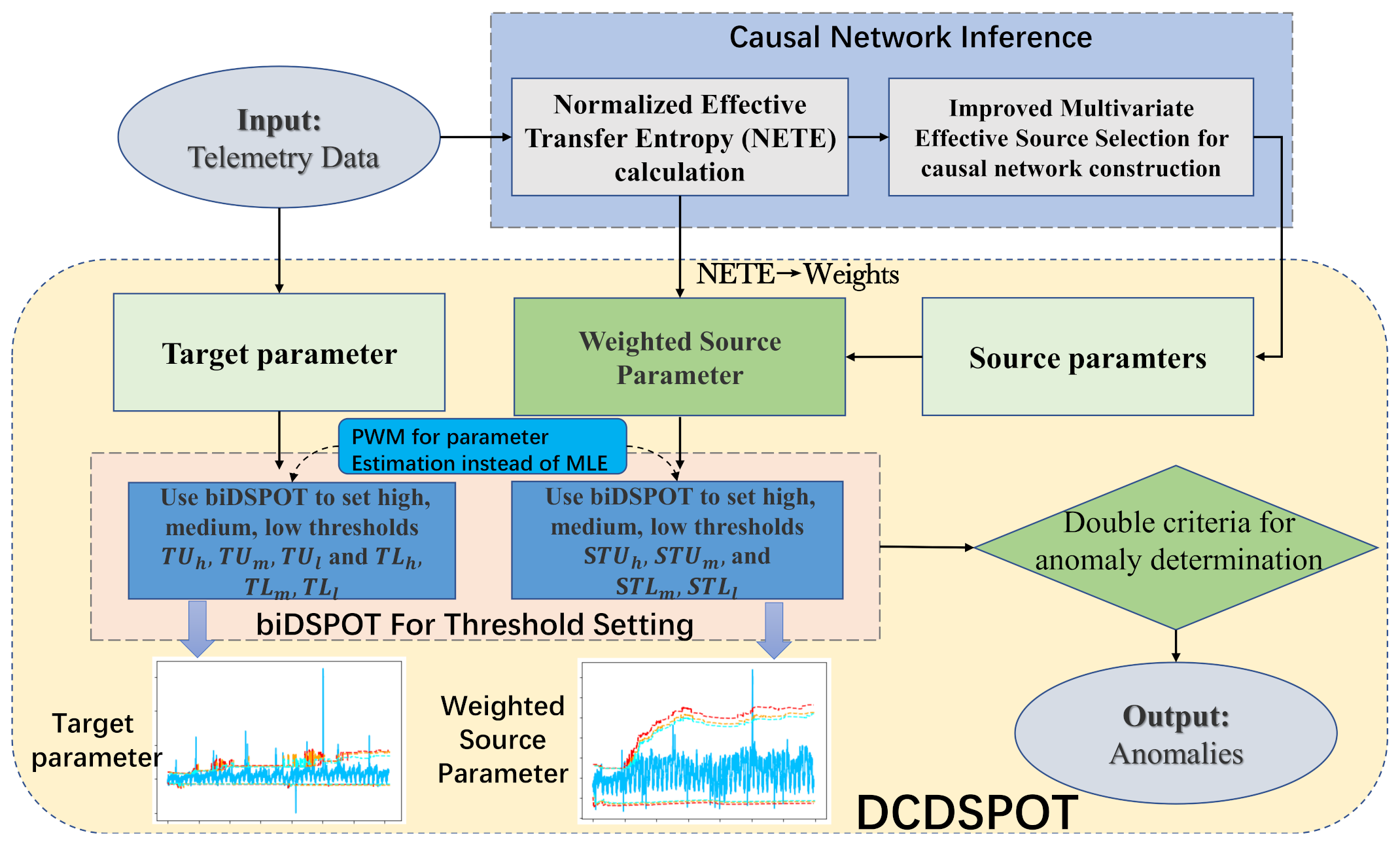
The framework of our method is shown in Figure 1.

Figure 1.
Framework of spacecraft telemetry anomaly detection based on parametric causality and double-criteria drift streaming peaks over threshold.
2. Related Work
In this section, we introduce the related works involved in our research. It mainly includes contents about spacecraft telemetry data anomaly detection, time series causal network inference, and POT and its derived methods.
2.1. Spacecraft Telemetry Data Anomaly Detection
During the spacecraft’s on-orbit operation, the sensor parameter information obtained by its internal operating status monitoring system is encoded and transmitted to the ground through the telemetry system. This telemetry data is the only basis for ground-based spacecraft operators to understand the spacecraft’s on-orbit operating status. If the on-orbit spacecraft is abnormal, the corresponding telemetry parameters’ trend will change. Hence, anomalies in telemetry data can reflect problems such as acquisition equipment failure, transmission link damage, quality problems, and mechanical and electronic failure.
Anomaly detection of the telemetry data is the key to realize the early warning of abnormal changes and effectively avoid possible failures. Anomaly detection is to use a certain method to realize the discovery of abnormal components in telemetry data. The anomaly types of telemetry data include point anomalies, contextual anomalies, collective anomalies, and correlated anomalies [13]. Recently, data-driven anomaly detection technology for spacecraft telemetry data has become a hot research topic, it does not require prior knowledge of expert experience, and it can detect anomaly through data analysis. Data-driven anomaly detection uses statistics, traditional machine learning or deep learning to model and characterize telemetry data to identify anomalous patterns that do not conform to normal data.
With the increasing number of on-orbit spacecrafts, the dimension of telemetry data that needs to be monitored in real time is expanding. Moreover, due to the different characteristics of anomalies and complex interaction in telemetry parameters, using data-driven methods to detect anomalies in telemetry data in a timely and effective manner has become more and more challenging. The problems of time-consuming methods, false negatives, and false positives commonly exist. Hence, detection methods with a high detection rate, low false detection rate, and strong interpretability have become a pressing need.
2.2. Time Series Causal Network
Telemetry data is essentially a multivariate time series with complex causality among its multiple parameters. Causality is more interpretable than correlation. Correlation only means "synchronized changes" of two variables, not directional, but causality means that a change in one variable will irreversibly affect another variable in some fixed pattern. Causality reflects not only the correlation in the aspect of statistics, but also the mutual influence in terms of physical mechanism or logic. Causality has been widely applied in many areas such as physics [14], biomedical science [15], ecosystems [16], and neuroscience [17].
Causal Bayesian Network (CBN) [18] represents a form of a time series causal network, and it is a specific version of Bayesian networks. A Bayesian network is based on the principles of Bayesian statistics, it is suitable for expressing and analyzing uncertain and probabilistic events. A Bayesian network uses the conditional probability to express the strength of the relationship, and uses the prior probability to express the information without a parent node. CBN is a Bayesian network that further stipulates that the edge between nodes indicates the causal relationship between two variables, the out-degree node of the edge denotes the cause variable (usually called source variable), and the in-degree node of the edge denotes the result variable (usually called the target variable).
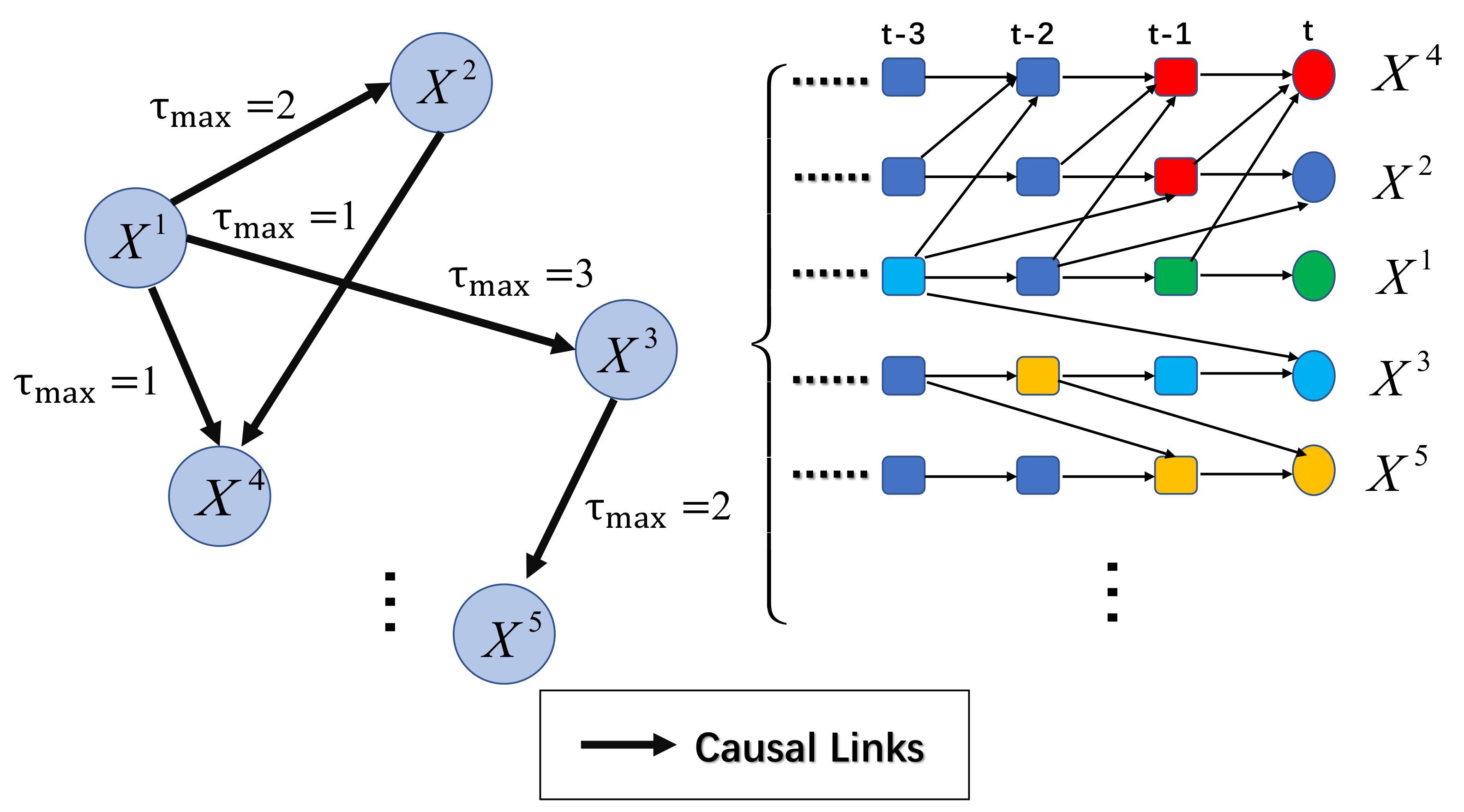
A time series causal network is a causal network that considers the causal relationship and time lag between variables. The Directed Acyclic Graph (DAG) denotes the time series causal network, and the node set denotes the set of variables. These variables are supposed to all be observable [19]. The set of directed edges denotes the causal relationship between nodes, and the causal time lag denotes the max time lags of causal relationships. Figure 2 shows an example of a time series causal network.
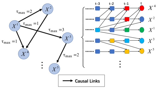
Figure 2.
An example of a time series causal network with five nodes and five edges. The arrows denote causal links, and denotes the max time lag of each causality.
Time series causal inference algorithms include methods based on regression analysis, methods based on information theory, and methods based on state space model [20]. Methods based on information theory can be applied to high-dimensional data as well as measuring the strength of the causality. Thus, they are widely used in time series causal inference. Schreiber et al. [21] proposed Binary Transfer Entropy (BTE) as a measure for causality strength. BTE can be used for non-linear data, but not for multivariate time series. Sun et al. [22] proposed Causal Entropy (CE) to measure causal strength. CE can be applied to multivariate time series and can also distinguish direct and indirect causality, but it cannot reflect the true causality strength. Hao et al. [23] proposed Normalized Causal Entropy (NCE), which can eliminate the indirect influence between nodes and measure the strength of causality more accurately than traditional methods by unifying dimension. However, for time series with a large amount of variables, its calculation complexity is high and it depends on prior knowledge. Runge [24] proposed the PCMCI (Peter Clark-Moment Conditional Independence) algorithm for constructing a causal network in a large scale multivariate time series. The algorithm is the improved version of the traditional PC (Peter Clark) algorithm. PCMCI removes false causality by adding an MCI test, but it has still not completely overcome the shortcomings of the PC algorithm, which has poor comprehensibility and robustness. Time series causal inference methods that are suitable for non-stationary, high-dimensional sequences, and can accurately reflect causal strength are the focus of current scholars.
2.3. Peaks over Threshold and Its Derived Methods
Siffer [12] proposed a POT method based on extreme value theory, which do not require manual threshold setting, and no assumptions are made on the distribution. POT is inspired by the Pickands-Balkema-de Haan theorem [25]. The POT approach tries to fit a Generalized Pareto Distribution (GPD) to the extreme values of , t is the initial “over-limit” threshold set as the high empirical quantile. Equation (1) shows that exceeding the initial threshold obeys the GPD with parameters , and , namely:
Here is a location parameter but set null, is a scale parameter, is a shape parameter, and the “+” signifies that if the expression in parentheses is negative then it should be replaced by 0.
Using the method proposed by Pickands [25] to estimate , , the final threshold is computed via Equation (2).
q is the risk parameter, n is the length of time series, is the number of peaks (that is, the number of ), is the updated threshold determined according to the confidence level , and Algorithm 1 shows the steps of POT.
| Algorithm 1 Peaks Over Threshold |
| Require: time series , risk parameter q, quantile |
| Ensure: |
| 1: function POT() |
| 2: # set by low quantile |
| 3: |
| 4: a method for the maximum likelihood estimation of parameter, see [26] |
| 5: |
| 6: return |
| 7: end function |
Besides, Siffer proposed Streaming POT (SPOT), Drift SPOT (DSPOT), bidirectional SPOT (biSPOT), and bidirectional DSPOT (biDSPOT) based on POT.
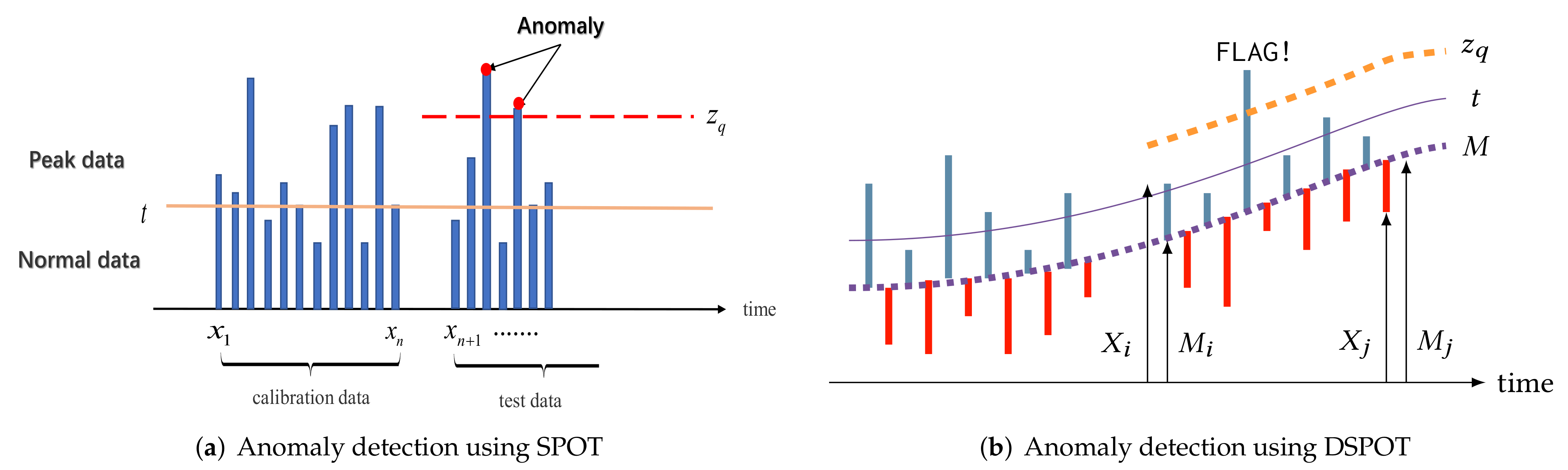
SPOT works in stationary cases assuming that the distribution of the does not change over time. The principle of the SPOT is the following: we want to detect abnormal events in a stream 0 in a blind way (without knowledge about the distribution). Firstly, we perform a POT estimate on the n first values and we get an initial threshold (initialization). Then, for all the next observed values we can flag the events or update the threshold (see Figure 3a). If a value exceeds threshold then we consider it as abnormal.
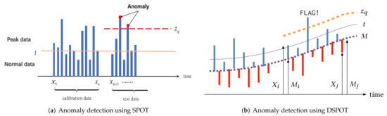
Figure 3.
Principles of anomaly detection using SPOT and DSPOT.
DSPOT takes a drift component into account to be applied in sequences with non-static distribution. DSPOT makes SPOT run not on the absolute values but on the relative ones , where models the local behavior at time i. with the last d “normal” values (see Figure 3b), d can be viewed as a window size.
SPOT and DSPOT can detect upper outliers but not lower outliers, so they may lead to a large number of false negatives. biSPOT and biDSPOT can effectively overcome the above shortcomings of SPOT and DSPOT. “bi” denotes “both sides”, which takes upper and lower thresholds updates into account.
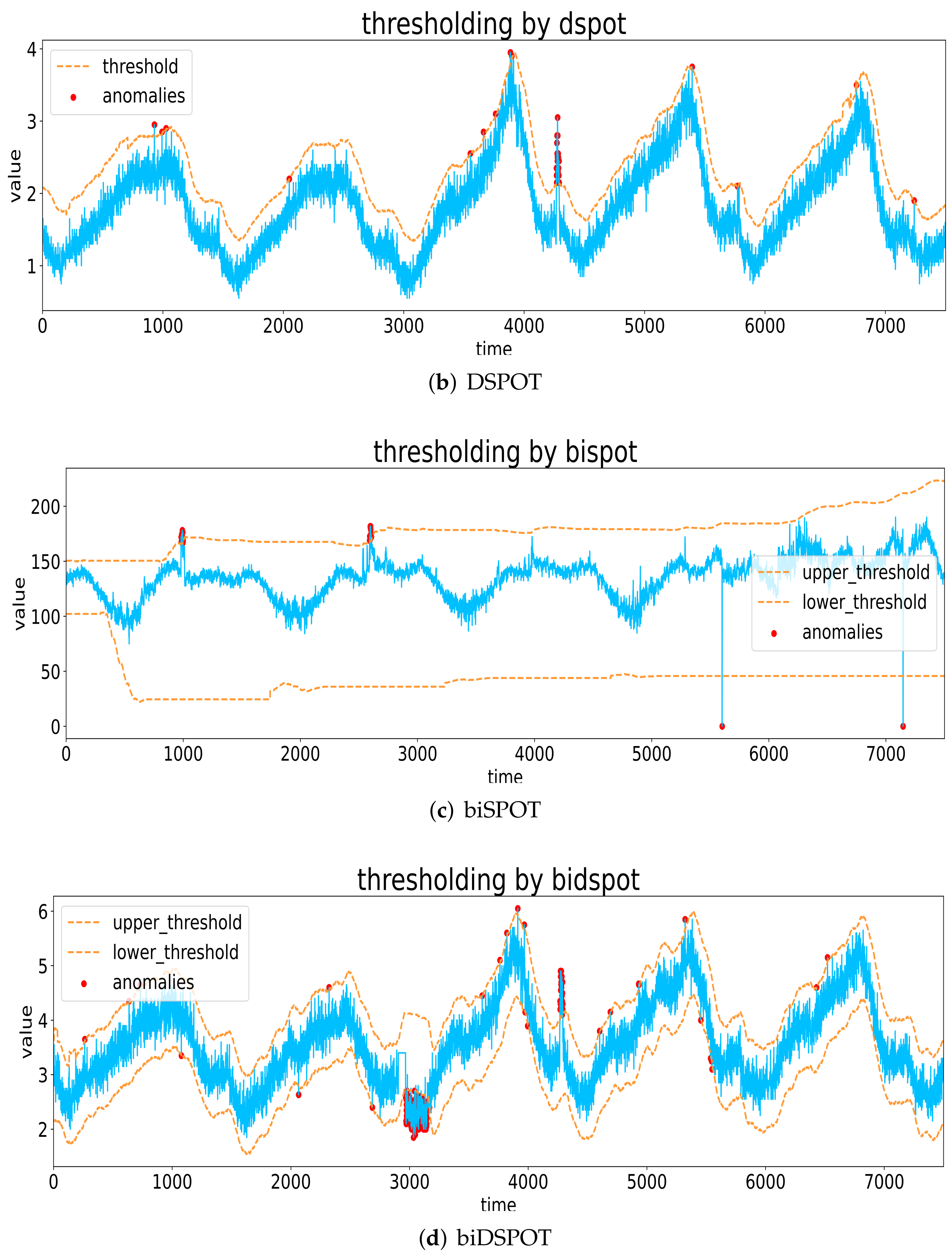
POT and its derived methods achieve outstanding performance in detecting extreme values without any label-related information, which has the potential to solve the unsupervised anomaly detection problem in large-scale time series. Figure 4 shows examples of anomaly detection using SPOT, biSPOT, DSPOT, and biDSPOT.
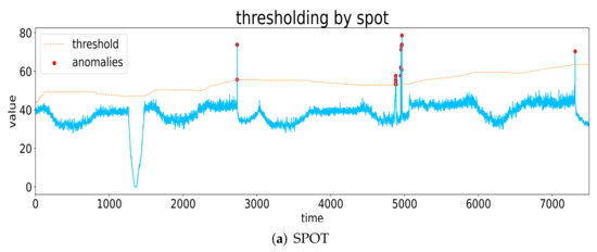

Figure 4.
Examples of anomaly detection using SPOT, biSPOT, DSPOT, and biDSPOT.
3. Causality Inference Using IMESS
In this section, we introduce a multivariate time series causal inference method based on Transfer Entropy (TE) and the Multivariate Effective Source Selection (MESS) algorithm. Then, we analyze the shortcomings of TE and propose a more reliable metric Normalized Effective Transfer Entropy (NETE) to overcome the defects of TE. Finally, we use NETE instead of TE to perform the MESS algorithm, which we call Improved MESS (IMESS).
3.1. Transfer Entropy
Transfer Entropy (TE) is a measure of causality for time series [19]. It can be intuitively interpreted as the current degree of uncertainty of X that is solved jointly by the variables X and Y and exceeds the current degree of uncertainty, which can be solved by X’s own past. Equation (3) gives the relationship between TE and Shannon entropy H, here .
denotes transfer entropy from Y to X, denotes Shannon information entropy, the subscript t denotes time, k and l denotes the embedding history length of X and Y, that is , has the same meaning. According to the calculation formula of Shannon entropy, Equation (4) gives the calculation of TE:
Generally, k is set as 1, l can be freely selected in practical applications, different l denotes different time lags of causality.
3.2. Multivariate Effective Source Selection
In a multivariate time series, the causality between variables are influenced by other parameters, resulting in a binary transfer entropy that cannot reflect the true flow of information between the two parameters. Lizier [27] proposed an algorithm named Multivariate Effective Source Selection (MESS), which can identify causality in multivariate time series.
Let be all variables in system, be the set of source parameters of X (), which is called the information contribution set. We can decompose into the collective transfer entropy of the previous t time-step information contribution set (denoted by ), the historical information provided by X itself (called Active Information Storage and denoted by ), and the inherent uncertainty or randomness information in X, as shown in Equation (5):
Equation (5) is called the information decomposition formula. According to the information decomposition formula, the source variables of a target variable is the set of variables that can incrementally provide enough information to reduce the uncertainty of the target variable. The steps of MESS are as follows:
- 1.
- Initialize .
- 2.
- For each possible source parameter , calculate .
- 3.
- Choose the that provides the largest incremental information contribution for the next state of X.
- 4.
- Repeat steps 2 and 3 until there is no Z that can be added to . The reason for the termination of the algorithm is that there is no more information in X left to account for, or no source Z provides a statistically significant information contribution which could account for part of the remaining uncertainty in X.
- 5.
- When no source Z can be found to provide a statistically significant information contribution , consider joint pair of sources instead of a single source Z, and repeat steps 2 and 3.
- 6.
- Once we have finalized the determination of after the above, then check whether each adds a statistically significant amount of information given all of the other sources selected for . Where the source fails this test, it is removed from .
3.3. Improved Multivariate Effective Source Selection (IMESS)
MESS has low computational complexity and can quickly determine causality in multivariate time series. The basis of the MESS is calculating the TE, but TE has two defects when it is used for causal inference:
- 1.
- The calculation of TE depends on the probability distribution of time series, which is affected by the non-stationarity and the noise of the data, and the limited sample effect can also easily lead to error of Shannon entropy estimation [19];
- 2.
- TE is affected by the amount of information of the variable, but the dimensions among different variables are not uniform, so that TE is not comparable. Even if there is no effective causal relationship between variables with large self-information, there might also be abundant information flow between them. Therefore, if the self-information gap of variables is too large, the accuracy of the causal inference algorithm based on TE will drop significantly.
Due to the two defects of TE above, causal inference based on MESS may lead to lots of false causalities. To overcome the defects of TE, we propose Normalized Effective Transfer Entropy (NETE). Before giving the definition of NETE, the definitions of Random Transfer Entropy (RTE) and Effective Transfer Entropy (ETE) are given below.
Definition 1 (Random Transfer Entropy (RTE)).
Randomly shuffle the time series of source variable for K times to break any causal relationship between variables, but keep the probability distribution of each time series unchanged, then calculate TE for each shuffling and take the average, which is the RTE.
denotes the sequence obtained by randomly shuffling X for the k-th time. RTE reflects the noise (error) caused by the non-timing of TE calculation, the non-stationarity of the data, and the finiteness of the scale of data. The value of K is generally set to be greater than 1000.
Definition 2 (Effective Transfer Entropy (ETE)).
ETE is the value that TE calculated by actual order of the data minus RTE, which reflects the “net” information transfer after eliminating the noise (error) caused by non-timing and non-stationarity of the data.
Definition 3 (Normalized Effective Transfer Entropy (NETE)).
NETE is the ratio of ETE to the Shannon entropy of the target variable. NETE considers the self-information of the target variable, and can unify the dimensions to a certain extent, so that it can measure the strength of causality more accurately.
Then we use NETE instead of TE as the basic metric for MESS to infer causality in multivariate time series. MESS based on NETE is called Improved MESS (IMESS) in our paper. Algorithm 2 shows the detailed steps of IMESS.
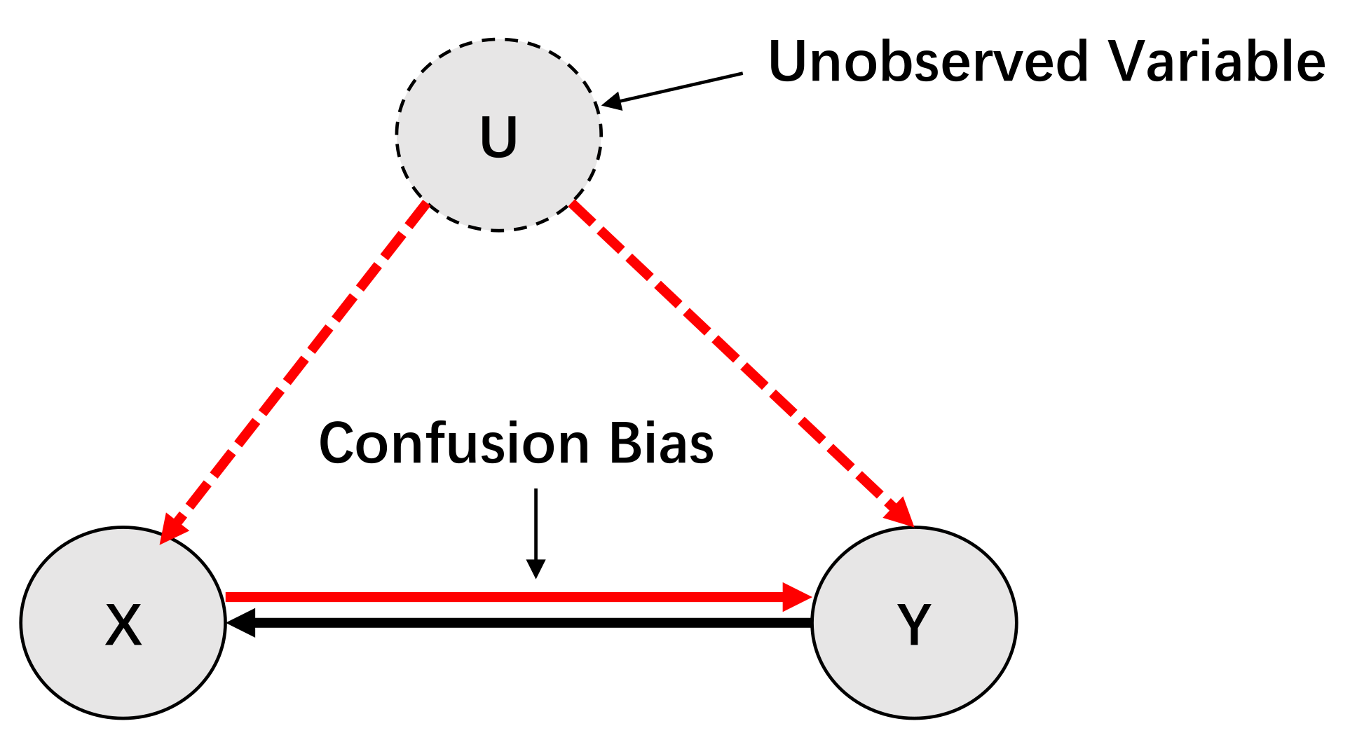
It should be noted that there might be bidirectional causalities of the network inferred by MESS and IMESS. They are logically unreasonable, but since we cannot observe all the variables in the system during causal inference, confusion bias is inevitable [28]. Bidirectional causality implies that there may be confusion bias caused by a hidden common cause (see Figure 5). Hence, in our study, bidirectional causality is considered to be reasonable.
| Algorithm 2: Improved multivariate effective source selection (IMESS) |
| Require: time series , target parameter |
| Ensure: (source parameters of ) |
| 1: function IMESS() |
| 2: |
| 3: repeat: |
| 4: for do |
| 5: calculate |
| 6: end for |
| 7: Add in |
| 8: until: |
| 9: No more information in left to account for OR no source Z provides a statistically significant information contribution which could account for part of the remaining uncertainty in |
| 10: repeat: |
| 11: for do |
| 12: calculate |
| 13: end for |
| 14: Add in |
| 15: until: |
| 16: no source provide a statistically significant information contribution which could account for part of the remaining uncertainty in |
| 17: for do |
| 18: if Z does not add a statistically significant amount of information given all of the other sources selected for then |
| 19: Remove Z from |
| 20: end if |
| 21: end for |
| 22: return |
| 23: end function |
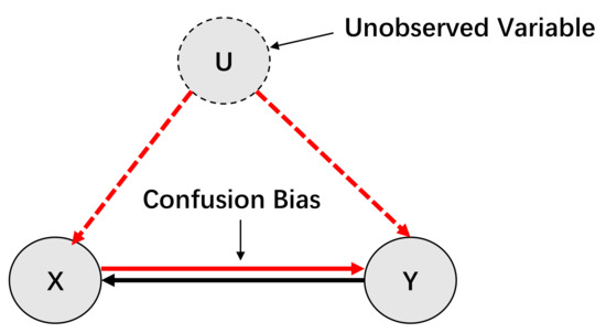
Figure 5.
An example of bidirectional causality. There is a causality Y→X. The variable U is an unobserved variable (or cannot measure), and there is causalities U →X and U →Y (U is the common cause of X and Y). However, since U cannot be observed, the information flow between U and X and U and Y may affect the information flow between X and Y, and since data-driven causal inference relies on conditional independence (conditional mutual information), which occurs when using the MESS algorithm, we may infer that X is the source variable of Y, and Y is also the source variable of X.
4. Double-Criteria Drift Streaming Peaks over Threshold (DCDSPOT)
POT and its derived methods have satisfying performance in univariate time series anomaly detection, but spacecraft telemetry data is multivariate, and there are complex interactions (causalities) among the parameters. These causalities tend to have a crucial impact on the anomalous patterns propagation of the parameters. To effectively take these causalities into consideration in anomaly detection, we propose a double-criteria anomaly detection method. Our method is improved on the basis of the DSPOT approach.
4.1. Weighted Source Parameter
Since causality exists universally in telemetry, when we aim to detect the anomaly of a certain target parameter, it is necessary to consider both the target parameter and its source parameters. In other words, we need to additionally take the values of source parameters of the target parameter into consideration when determining whether the target parameter is abnormal.
When we apply causality to detect anomalies of a target parameter, whether it is anomalous or not cannot be inferred merely based on the value of a certain source parameter or part of the source parameters. There are two reasons. First, some variables that have non-negligible impact on the system exist but we cannot observe them (or it is difficult to be accurately measured), such as the intensity of sunlight in the spacecraft system. Therefore, the source parameters we select may be only part of all the source parameters, and the anomaly of one source parameter does not inevitably cause the anomaly of the target parameter. Second, although the interactions among some source parameters and the target parameter are not significant, their extreme anomalous mode may also lead to anomaly of the target parameter. Hence, we need to comprehensively consider the influence of all source parameters on target parameter.
Suppose the target parameter is , and all its source parameters are , the time lags of all causalities are . When we are detecting the value of the target parameter at time t, we need to take the value of the source parameter at time () into consideration, because if the anomalous mode appears in at time t, it will not spread to target parameter until time . When t is less than , we take as a substitute for .
Then we define the Weighted Source Parameter (WSP), which is denoted by . WSP is a “virtual” parameter weighted and summed according to the strength of the source parameters’ influence (value of NETE in our method) on the target parameter (see Equation (10). Equation (9) shows the mathematical definition of WSP, and the negative sign in superscript means the timestep moves backward. WSP does not actually exist, but it represents the weighted synthesis of the numerical modes of all the source parameters. The extreme value distribution of WSP can also be regarded as approximately obeying GPD [29].
denotes shifting the sequence backward by , that is .
4.2. Multi-Tier Thresholds
The original threshold-based anomaly detection often sets a single threshold. Once the threshold is exceeded, the value here is determined to be an anomaly, such as setting threshold based on threshold library [30], setting threshold based on expert experience [31], 3 criterion, and mixture Gaussian distribution [32]. The original methods are simple and fast, but they have poor robustness, because the setting of the threshold is not completely automatic, some risk parameters (such as q in SPOT) need to be set manually, and the selection is often subjective and instable. To enhance the robustness, we introduce multi-tier thresholds based on biDSPOT, which is suitable for multivariate time series.
First, we define the high-tier, medium-tier, and low-tier thresholds , , and of the target parameter. is the limit of the threshold, once the value of the target parameter exceeds , then it can be concluded to be an anomaly. is a safety threshold, and if the value of the target parameter does not exceed , it can be concluded that it is not an anomaly. can be regarded as an “alarm” threshold, when the value of the target parameter exceeds , it is likely to be anomalous.
The “high-tier, medium-tier, and low-tier” thresholds mentioned above are applicable to anomaly detection of “exceeding upper limit”. To detect values that exceed low limit, we use lower thresholds denoted by , , and . All thresholds are computed using the biDSPOT by setting different risk parameters (see Equation (11)).
, ,and denote high, medium, and low risk parameters, and . The reason for using the last two sub-equations in Equation (11) is that due to the error of parameter estimation, the threshold computed by does not necessarily lead to , so we need to reorder them to get the result we want. “” means to find the maximum, minimum, and median of numbers. denotes using Algorithm 1 and methods illustrated in Section 2.3 to compute upper and lower thresholds.
Similarly, we can also define high-tier, medium-tier, and low-tier thresholds for the WSP. The “exceeding upper limit" thresholds are denoted by , , and . The “exceeding low limit" thresholds are denoted by , , and .
, , and denote high, medium, and low risk parameters, and . Generally, we set . For WSP, we only need two tiers of threshold, but we still compute the thresholds using three risk parameters, because we must ensure that the thresholds of target parameter and WSP are determined at the same risk levels.
In order to detect anomaly according to the multi-tier thresholds, we formulate two criteria for WSP and target parameter, which are given in Table 1. When the values of target parameter and the WSP meet the two criteria respectively at the same time, the value of the target parameter is judged to be an anomaly.

Table 1.
Anomaly cases determined by double-criteria and multi-tier thresholds.
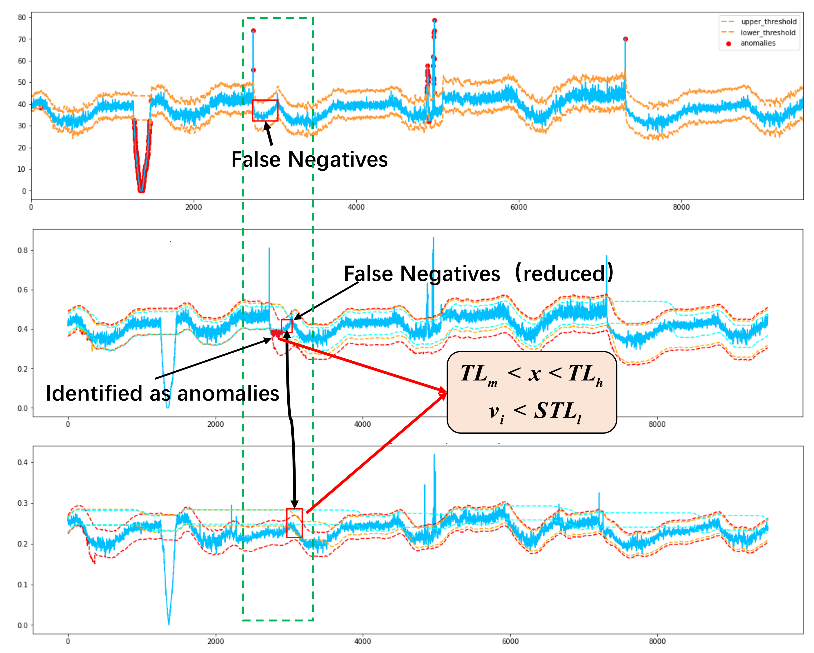
The method of setting multi-tier thresholds based on biDSPOT and using two criteria to identify anomaly is called Double-Criteria DSPOT (DCDSPOT). DCDSPOT considers the target parameter and the source parameters at the same time, which can reduce the false detection caused by the instability and noise of the target parameter during anomaly detection. As a result, the performance of DCDSPOT in reducing false negatives is outstanding. Figure 6 shows a case of anomaly detection by DCDSPOT, Figure 7 compares the biDSPOT and DCDSPOT methods and shows how DCDSPOT eliminates false negatives.
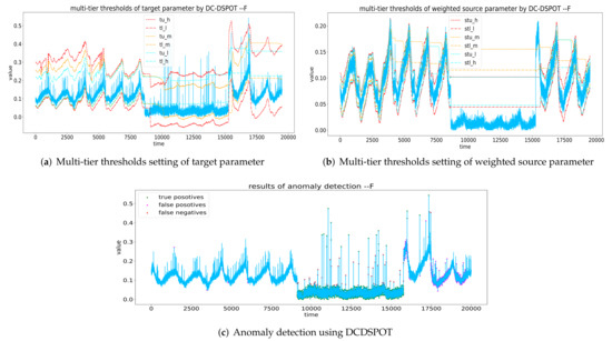
Figure 6.
An example of anomaly detection using DCDSPOT. In the first and second sub-figures, the red curve represents thresholds calculated by and , the orange curve represents thresholds calculated by and , and the light blue curve represents thresholds calculated by and .
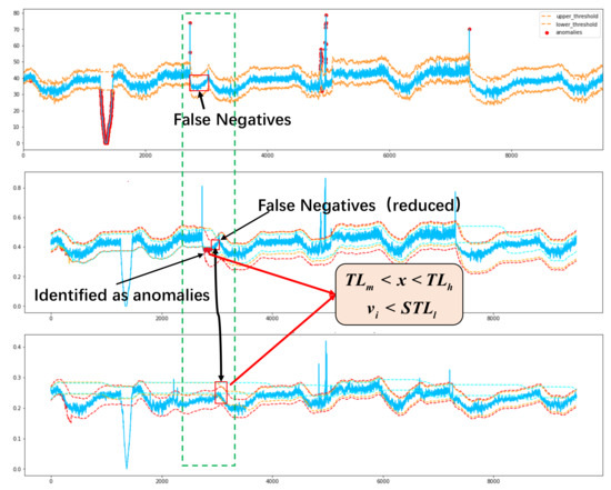
Figure 7.
A case that illustrates how DCDSPOT eliminates false negatives. A sequence is judged as normal by biDSPOT, but these are false negatives. By setting multi-tier thresholds for WSP and target parameter, false negatives that meet and are corrected.
4.3. Probability Weighted Moments for Parameter Estimation of GPD
When we employ DCDSPOT for anomaly detection, it is inevitable to set three different thresholds for the target parameter and the WSP. Hence, the running time is 6 times that of the original biDSPOT. To shorten the running time of our method, parameter estimation needs to be improved.
Parameter estimation using the Maximum Likelihood Estimation (MLE) method is time-consuming. In our method, we applied Probability Weighted Moments (PWM) for parameter estimation of GPD instead of MLE by Grimshaw trick [26]. PWM is based on the basic principle of the moment estimation method, which regards the probability distribution as the weights. The formula of PWM is described in Equation (13):
denotes r-order probability weighted moment, and denotes the parameter of the distribution function, and means to find the expected value. Substituting the GPD function into Equation (13), the r-order PWM of the GPD distribution can be calculated via Equation (14):
can be estimated by Equation (15) using the sample:
where , that is, denotes the i-th data in the sequence after arranging the sample data from small to large. Then and can be computed via Equation (16):
Finally, the sample PWM is used instead of the population PWM to estimate parameters, namely:
In our method, we use Algorithm 3 to calculate thresholds of POT.
| Algorithm 3 Peaks over threshold Using PWM |
| Require: time series , risk parameter q, quantile |
| Ensure: |
| 1: function POT using PWM() |
| 2: # set by low quantile |
| 3: |
| 4: Equation (17) |
| 5: |
| 6: return |
| 7: end function |
5. Case Study
In this section, to verify the novelty and effectiveness of our method in causal inference and anomaly detection, we conduct comparative experiments on two datasets with known causality and a satellite telemetry dataset.
5.1. Causal Network Inference Experiment
To verify the effectiveness on causal inference of IMESS algorithm, we employ two datasets with known causal relationships to conduct comparative experiments. In the experiment, three advanced algorithms of PCMCI, NCE, and MESS are used as the baseline algorithms to be compared with IMESS.
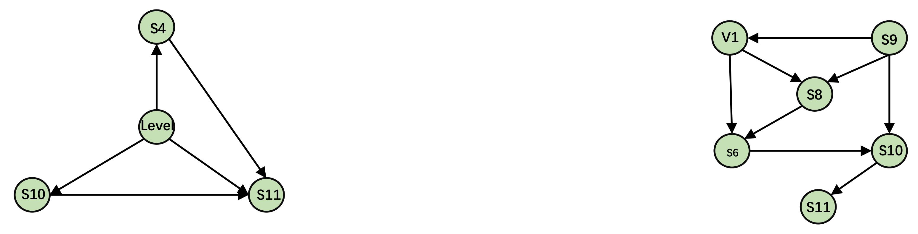
We selected two datasets in Refs. [33,34] for experimental verification, which are denoted by Dataset1 and Dataset2, respectively. The true causal relationships in these two datasets are shown in Figure 8. Dataset1 comes from the physical system of the network, and Dataset2 comes from the industrial system.
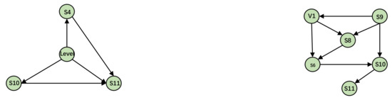
Figure 8.
Real causal network of Dataset1 and Dataset2.
In our experiment, MESS and IMESS may infer bidirectional causality, and when bidirectional causality is inferred, we choose the causality with greater as the final direction of causality, which is also logical.
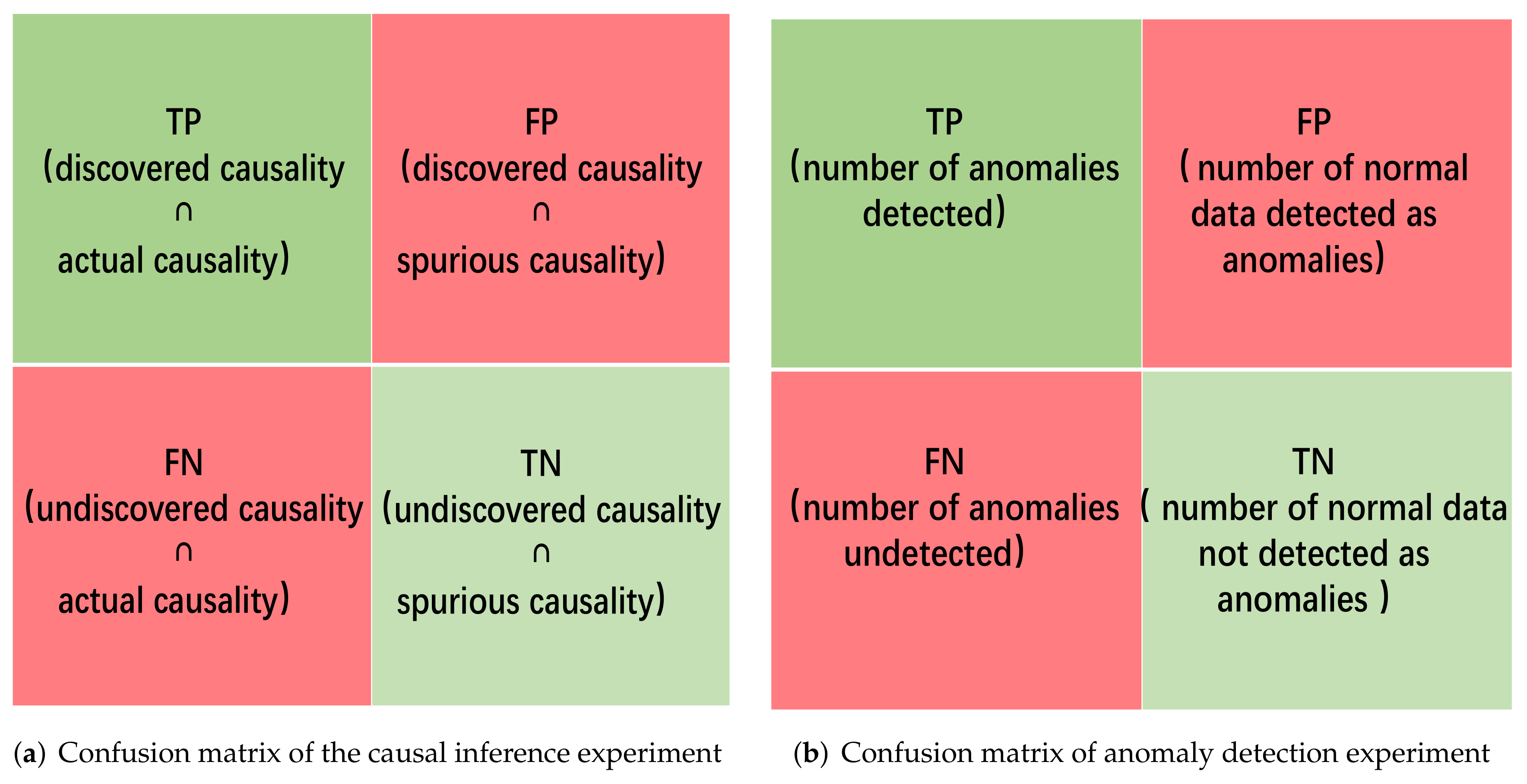
Three evaluation metrics, recall, precision, and F1-score, are introduced to evaluate the performance of the algorithm. Recall is used to measure undiscovered edges between nodes. Precision is used to measure edges that do not exist in the causal network graph that are added by mistake. F1-score is a combination of recall and precision that can evaluate the integrated performance of the causal network inference algorithm. Figure 9a shows the confusion matrix of causal inference experiment, Equation (18) gives the definition of the three metrics.
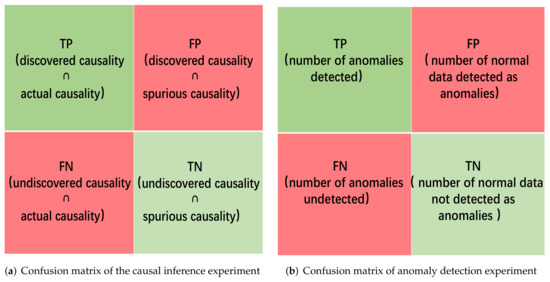
Figure 9.
Confusion matrix of the anomaly detection experiment.
Figure 10 shows the inference results of the baseline algorithms and IMESS on two datasets. Table 2 shows the precision, recall, and F1-score of these causal inference algorithms. It should be noted that all four algorithms need to manually set the confidence level of the significance test or conditional independence test (which can be regarded as the “hyperparameters” of the algorithm), the inference results will also change with these hyperparameters. Therefore, we selected the results closest to the true causal network by grid search among all the results of the four causal inference algorithms for comparison. It can be concluded that IMESS has a higher F1-score than the baseline algorithms.
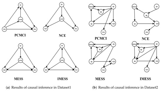
Figure 10.
Causal inference results of IMESS and three baseline algorithms on Dataset1 and Dataset2.
Table 2.
Performance comparison between IMESS and three baseline algorithms.
5.2. Parametric Causality Inference and Anomaly Detection on a Real Satellite Telemetry Dataset
5.2.1. Telemetry Dataset
To verify the performance of our method in spacecraft telemetry anomaly detection, we select a real satellite for the experiment. The name of this satellite is “Satellite A”. Satellite A is a military communication satellite, it enables any ground, sea and air communication stations in the coverage area to communicate with each other at the same time, and has the function of transmitting information such as telephone, telegram, fax, data, and television. The telemetry dataset of satellite A contains more than 20 telemetry parameters, and the labels of anomalies are given by experts and the operation system of the satellite. For the purpose of confidentiality, we do not give the actual meaning of each telemetry parameter in this satellite. Instead, we use A, B, C, … T to indicate them. Our satellite telemetry data has been declassified through normalization and uploaded together with the paper (named “experiment data.csv”). Among these parameters, B, D, Q, and T are are the important parameters summed up by most experts and engineers in the long-term satellite anomaly detection task based on the basic structure and design principles of the satellite. These parameters have a crucial impact on the normal operation of the satellite. Parameter B represents the output power of the southern solar array, parameter D represents the output power of the northern solar array, parameter Q represents the shell temperature of the transponder, and parameter T represents the bearing shell temperature of the momentum wheel. The dataset has 67,968 items of data sampled in 236 days, and the sampling interval is 5 min. Table 3 gives the basic information of this satellite telemetry dataset.
Table 3.
Basic information of the satellite telemetry dataset.
5.2.2. Parametric Causal Network Inference
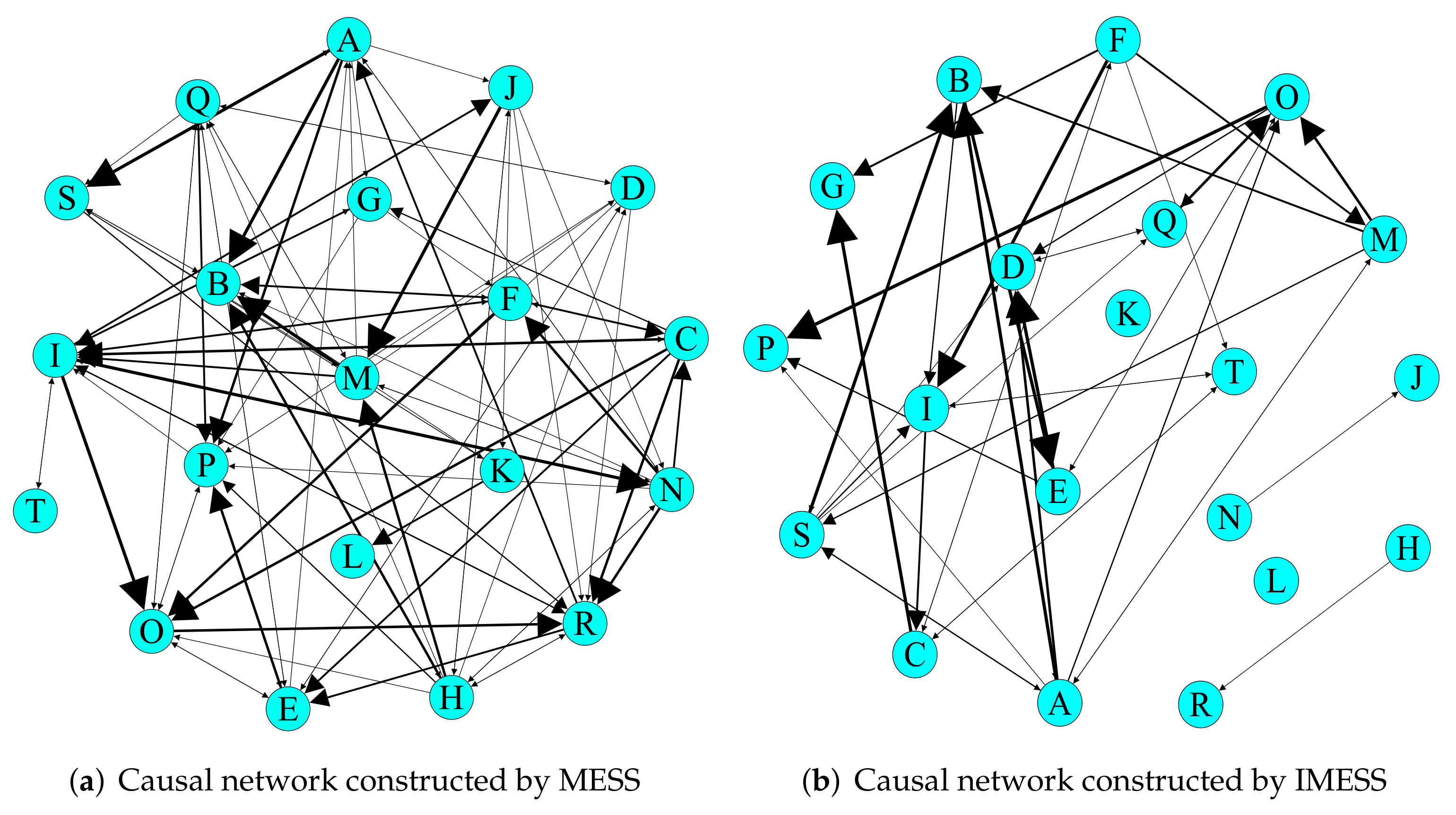
In this section, we applied MESS and IMESS for parametric causal network inference. Similarly, we employ precision, recall, and F1-score as the evaluate metrics of (see Equation (18)). Figure 11 shows the parametric causal network inferred by MESS and IMESS. Table 4 shows all the target parameters and their corresponding source parameters of all causalities. Regarding the inferred causalities, we verify the reliability by analyzing the physical properties the parameters represented and consulting experts in satellite development, design, operation, and maintenance. After comprehensive analysis, combined with the experimental results of Section 5.1, we have reason to believe that the causality inferred by IMESS is reliable and more reasonable than that of MESS (although we do not know the true mechanism of the satellite system and causality of these parameters).

Figure 11.
Parametric causal network inferred by MESS and IMESS. MESS leads to 95 edges, and IMESS leads to 43 edges. The width of the edge in the causal network represents the maximum causal time lag.
Table 4.
Target parameters and corresponding source parameters with maximum causal time lags.
5.2.3. Anomaly Detection
To verify the performance on telemetry anomaly detection of our method, we compare it with biSPOT and biDSPOT methods to verify the improvement. The 3, Local Outlier Factor (LOF) [35], One-class support vector machine (OCSVM) [36], and Isolation Forest [37] methods also serve as baselines, all of which do not require predicting the telemetry data. Furthermore, we compare our method with three data-driven anomaly detection methods based on prediction models, Long Short-term Memory-Variance Auto Encoder (LSTM-VAE) [38], Generative Adversarial Networks (GAN) [39], and Temporal Convolutional Network (TCN) [40].
We employ precision, recall, and F1-score as the evaluate metrics (see Equation (18)). Figure 9b shows the confusion matrix of anomaly detection experiment. We also recorded the time-consumption of each method in the anomaly detection phase (experimental environment configuration: Windows 10 + python 3.8 + CUDA 10.1 + CUDNN 7.6.5 + tensorflow 2.5.0).
When using biSPOT, biDSPOT, and DCDSPOT for anomaly detection, the setting of the risk parameter and are very critical, because they directly affect the detection effect. In Ref. [12], q is manually set to be and , but in actual application, we need to determine the most reasonable q value based on historical detection results. In our experiment, value of q is selected by hyperparameter optimization, that is, we use grid search to find the q that can achieve the best detection performance. For different target parameter sequences, the optimal q settings are different, because these parameters have different operating modes. The parameter d of DSPOT is also determined by the same approach.
When applying LSTM-VAE, GAN, and TCN for anomaly detection, it is necessary to set thresholds for residual to determine whether a value is anomalous. We use the SPOT to set thresholds for the residual sequence, because the residual sequence is often considered stable.
5.2.4. Results and Discussion
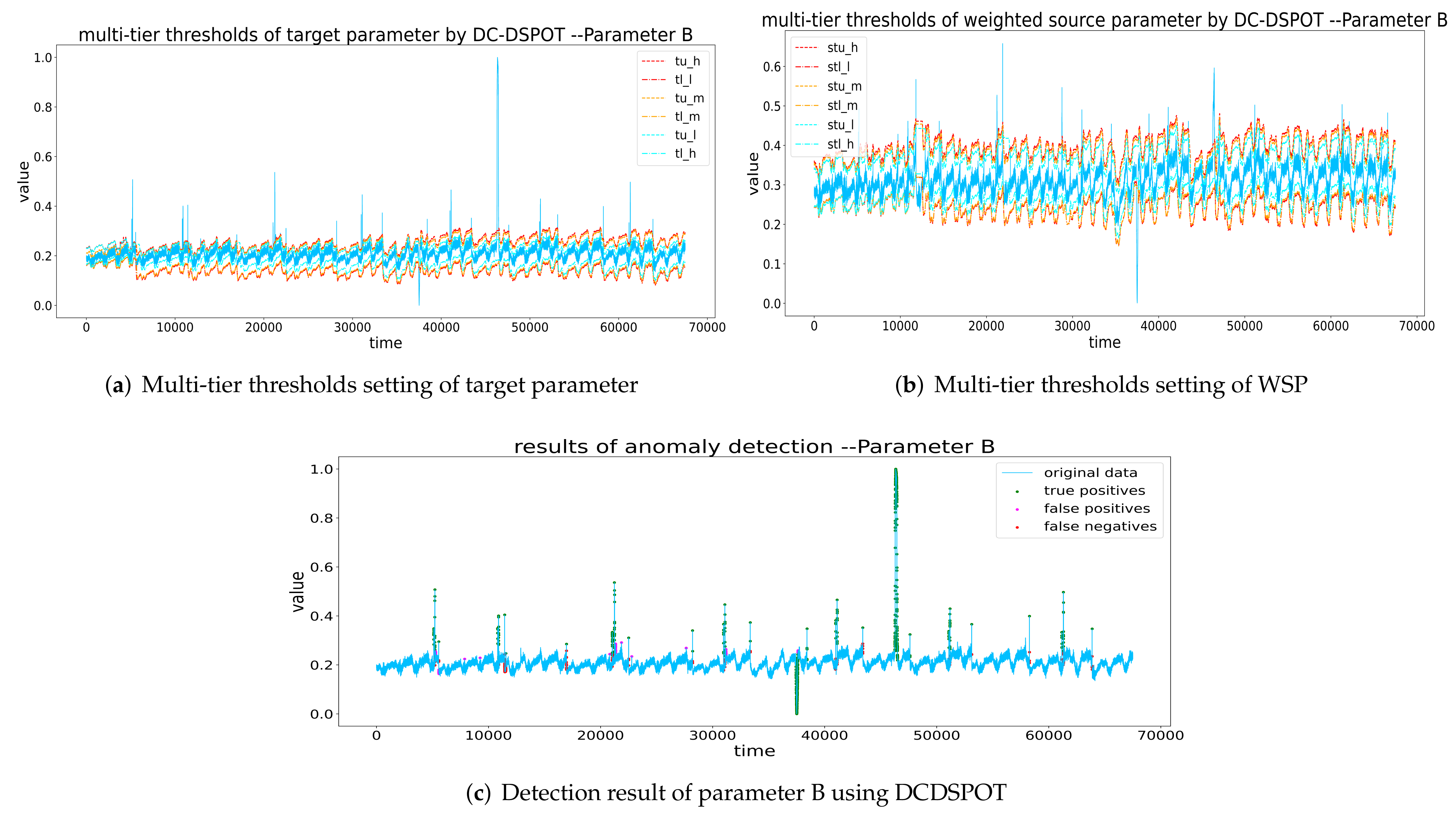
Figure 12, Figure 13, Figure 14 and Figure 15 show the multi-tier thresholds setting and anomaly detection result of the four target parameters using DCDSPOT. Table 5 shows the precision, recall, F1-score, and running time of DCDSPOT and the baseline methods.
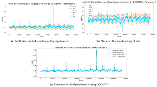
Figure 12.
Thresholds setting and detection result of B by DCDSPOT. (a,b) The multi-tier thresholds setting of the target parameter and WSP (the red dashed line is , the orange dashed line is the , and the blue dashed line is the ), and (c) the detection results of DCDSPOT.
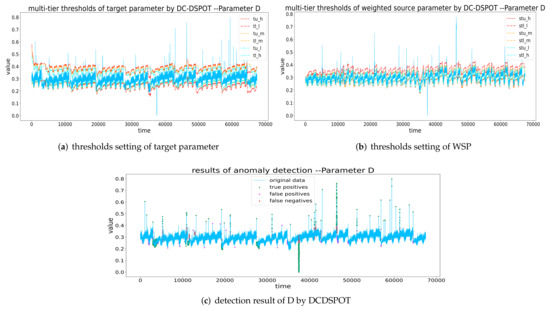
Figure 13.
Thresholds setting and detection result of D by DCDSPOT. (a,b) The multi-tier thresholds setting of the target parameter and WSP (the red dashed line is , the orange dashed line is the , and the blue dashed line is the ), and (c) the detection results of DCDSPOT.
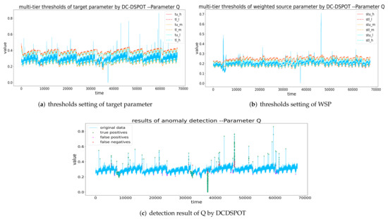
Figure 14.
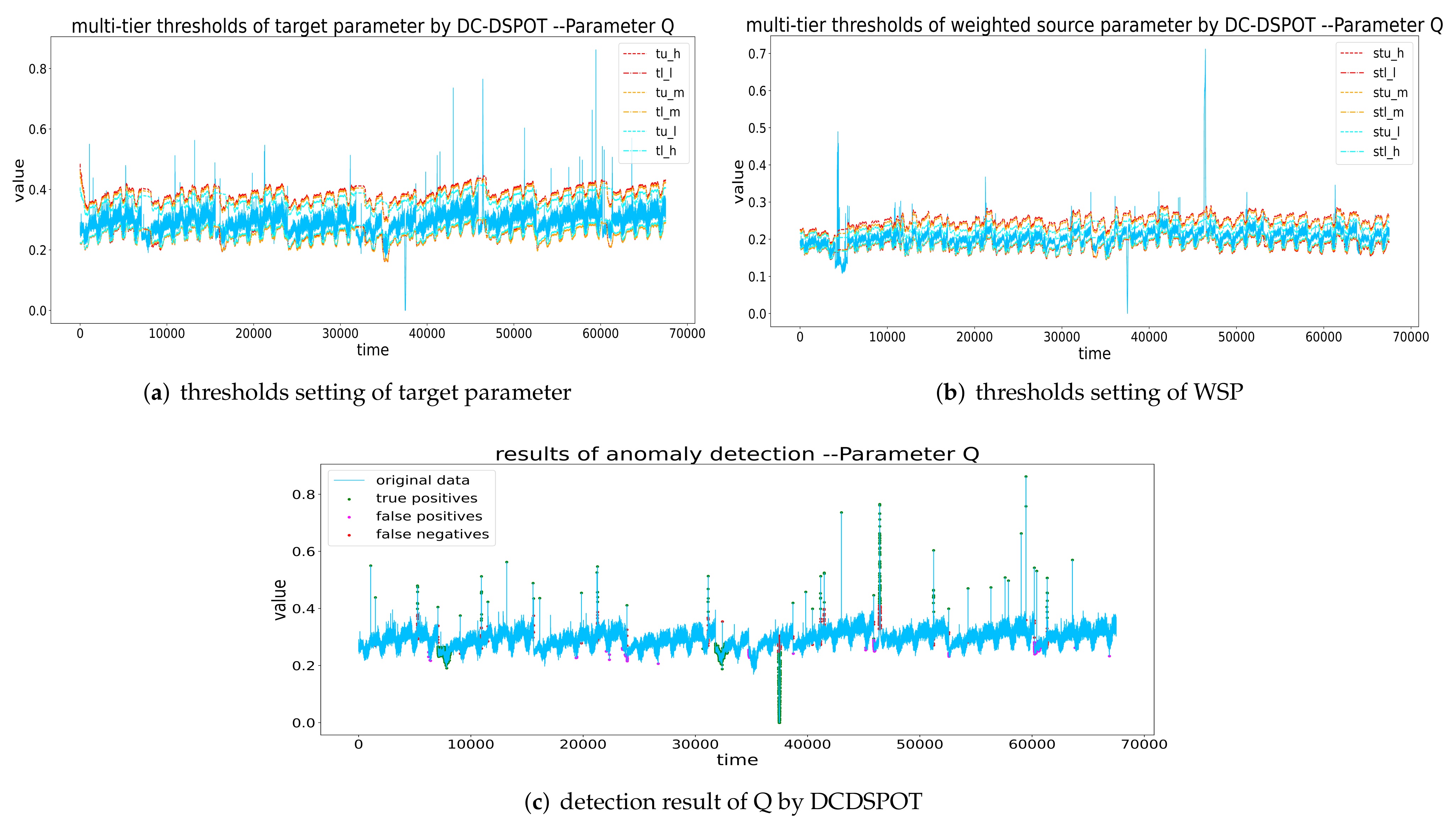
Thresholds setting and detection result of Q by DCDSPOT. (a,b) The multi-tier thresholds setting of the target parameter and WSP (the red dashed line is , the orange dashed line is the , and the blue dashed line is the ), and (c) the detection results of DCDSPOT.
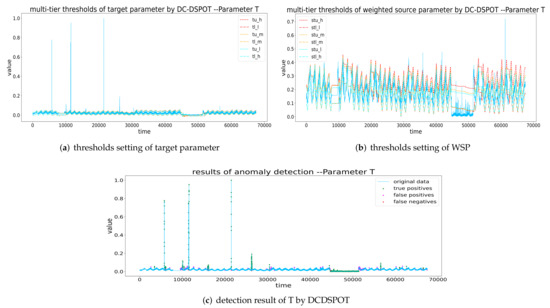
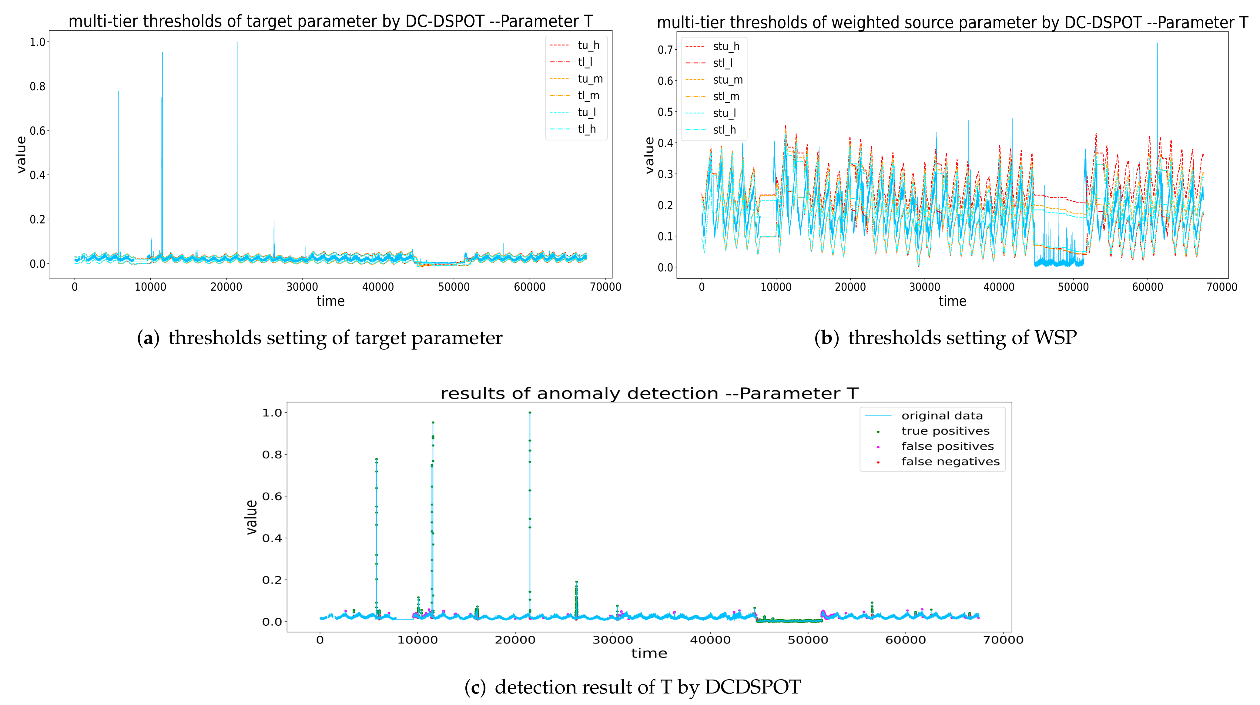
Figure 15.
Thresholds setting and detection result of T by DCDSPOT. (a,b) The multi-tier thresholds setting of the target parameter and WSP (the red dashed line is , the orange dashed line is the , and the blue dashed line is the ), and (c) the detection results of DCDSPOT.
Table 5.
Anomaly detection performance of baseline methods and DCDSPOT.
Our method and similarity-based methods and other statistical model-based methods. It can be concluded that the recall and F1-score of the DCDSPOT method are significantly higher than those of the baseline methods of 3, LOF, OCSVM, Isolation Forest, biSPOT, and biDSPOT. However, DCDSPOT takes a longer running time compared with them. The reason why DCDSPOT has a higher recall rate (lower false negative rate) is that it fully considers all other factors in the telemetry system that have a significant impact on target detection parameters. Moreover, our method determines anomalies by taking the propagation effects of anomalous data patterns into consideration. For example, items 3371–4431 of parameter D are anomalies, but it is difficult to detect them merely based on the data of the target parameter (which can be achieved by setting lower risk parameters, but there will be many false positives). However, these anomalies can be determined by analyzing D and D’s weighted source parameter. All in all, by setting multiple thresholds and comprehensively analyzing the weighted source parameters and target parameter, DCDSPOT can effectively reduce false positives and false negatives.
Our method and prediction model-based methods. Anomaly detection based on prediction models has lower precision and recall than our method, which is mainly due to the error of the prediction models. In addition, they are more time-consuming because a good prediction model requires multiple epoch of iterations. Another shortcoming of anomaly detection methods based on prediction model is that they may learn anomalous patterns after encountering anomalies with a long duration, which makes the model no longer sensitive to anomalies (see the anomaly detection of parameter T). By contrast, DCDSPOT has higher recall and F1-score than anomaly detection methods based on prediction models, and it can better identify long sequential anomalies.
Precision of our method. Compared with some baseline methods, DCDSPOT has lower precision. The reason is that in order to reduce false negatives as much as possible, the multi-tier risk parameters need to be set lower, which will inevitably lead to more false positives (lower precision). However, the degree of recall improvement is much higher than that of precision reduction, so the F1-score is improved significantly. The F1-score is a comprehensive metric of anomaly detection, and it is also the metric we pay more attention to.
Comparison of detection time complexity using PWM and MLE. Furthermore, to improve the performance of time complexity of DCDSPOT, we replace Grimshaw trick based MLE with PWM to estimate the parameters of GPD and to set the thresholds. It can be seen from Table 6 that the detection performance of DCDSPOT using PWM and DCDSPOT using MLE is not much different, but that the running time is shortened by 4–5 times, which proves that the method we proposed is efficient in reducing time complexity.
Table 6.
Anomaly detection performance of PWM-based DCDSPOT and MLE-based DCDSPOT.
6. Conclusions and Future Work
To solve the problems of high false negatives, long time consumption, and poor interpretability of spacecraft telemetry data anomaly detection methods based on statistical model, an anomaly detection method based on parametric causality and Double-Criteria DSPOT (DCDSPOT) is proposed in this paper. Normalized Effective Transfer Entropy (NETE) is proposed to remove errors and noise in the calculation of transfer entropy so as to improve the MESS algorithm. An experiment on two datasets with known causality verifies that the F1-score of causality inference using Improved MESS is significantly improved. DCDSPOT is proposed for thresholds setting of target parameters to be detected and the Weighted Source Parameter (WSP), then two criteria are formulated to determine the anomaly of the target parameter. Furthermore, to mitigate the time-consumption problem of DCDSPOT, we use PWM instead of MLE to estimate the parameters of GPD to set the thresholds. An experiment on a real satellite shows that our method has better performance on recall, F1-score, and running time.
Causality is common in the parameters of spacecraft systems, and it also plays an important role in anomaly detection and fault diagnosis of spacecrafts. In future research work, the authors will further study and improve the causal inference algorithm of telemetry parameters, the method of fault root cause diagnosis, and especially the combination of causality and advanced deep learning methods (such as LSTM, Graph Neural Networks, Transformer, etc.), so as to develop methods to detect different types of anomalies and better monitor the health status of the spacecraft and effectively maintain the system.
Author Contributions
Conceptualization, G.J.; methodology, Z.Z. and S.C.; software, C.X.; validation, Z.Z.; investigation, Z.Z.; resources, S.C. and L.Z.; data curation, Z.Z.; writing—review and editing, C.X.; visualization, Z.Z.; supervision, G.J. All authors have read and agreed to the published version of the manuscript.
Funding
This research received no external funding.
Conflicts of Interest
The authors declare no conflict of interest.
Abbreviations
The following abbreviations are used in this manuscript:
| TE | Transfer Entropy |
| RTE | Random Transfer Entropy |
| ETE | Effective Transfer Entropy |
| NETE | Normalized Effective Transfer Entropy |
| MESS | Multivariate Effective Source Selection |
| IMESS | Improved Multivariate Effective Source Selection |
| POT | Peaks Over Threshold |
| SPOT | Streaming Peaks Over Threshold |
| DSPOT | Drift Streaming Peaks Over Threshold |
| DCDSPOT | Double-Criteria Drift Streaming Peaks Over Threshold |
| MLE | Maximum Likelihood Estimation |
| MoM | Method of Moment |
| PWM | Probability Weighted Moment |
References
- Darvish, K.; Pourtakdoust, S.H.; Assadian, N. Linear and nonlinear control strategies for formation and station keeping of spacecrafts within the context of the three body problem. Aerosp. Sci. Technol. 2015, 42, 12–24. [Google Scholar] [CrossRef]
- Zheng, Z.; Jian, G.; Eberhard, G. Onboard mission allocation for multi-satellite system in limited communication environment. Aerosp. Sci. Technol. 2018, 79, S1270963818301287. [Google Scholar] [CrossRef]
- Hendricks, R.; Eickhoff, J. The significant role of simulation in satellite development and verification. Aerosp. Sci. Technol. 2005, 9, 273–283. [Google Scholar] [CrossRef]
- Miao, Y.; Hwang, I.; Liu, M.; Wang, F. Adaptive fast nonsingular terminal sliding mode control for attitude tracking of flexible spacecraft with rotating appendage. Aerosp. Sci. Technol. 2019, 93, 105312. [Google Scholar] [CrossRef]
- Zhang, C.; Wang, J.; Zhang, D.; Shao, X. Learning observer based and event-triggered control to spacecraft against actuator faults. Aerosp. Sci. Technol. 2018, 78, 522–530. [Google Scholar] [CrossRef]
- Weizheng, L.I.; Meng, Q. Fault Detection for in-orbit Satellites Using an Adaptive Prediction Model. Chin. J. Space Sci. 2014, 34, 201–207. [Google Scholar]
- Peng, X.; Pang, J.; Peng, Y. Review on anomaly detection of spacecraft telemetry data. Chin. J. Sci. Instrum. 2016, 37, 17. [Google Scholar]
- An, J.; Cho, S. Variational Autoencoder based Anomaly Detection using Reconstruction Probability. Comput. Sci. 2015, 2, 1–18. [Google Scholar]
- Nikolay Laptev, S.A.; Flint, I. Generic and scalable framework for automated time-series anomaly detection. In Proceedings of the 21th ACM SIGKDD International Conference on Knowledge Discovery and Data Mining, Sydney, Australia, 10–13 August 2015; pp. 1939–1947. [Google Scholar]
- Liu, D.; Zhao, Y.; Xu, H.; Sun, Y.; Pei, D.; Luo, J.; Jing, X.; Feng, M. Opprentice: Towards practical and automatic anomaly detection through machine learning. In Proceedings of the 2015 Internet Measurement Conference, Tokyo, Japan, 28–30 October 2015; pp. 211–224. [Google Scholar]
- Xu, H.; Feng, Y.; Chen, J.; Wang, Z.; Qiao, H.; Chen, W.; Zhao, N.; Li, Z.; Bu, J.; Li, Z. Unsupervised Anomaly Detection via Variational Auto-Encoder for Seasonal KPIs in Web Applications. In Proceedings of the 2018 World Wide Web Conference, Lyon, France, 23–27 April 2018. [Google Scholar]
- Siffer, A.; Fouque, P.A.; Termier, A.; Largouet, C. Anomaly Detection in Streams with Extreme Value Theory. In Proceedings of the ACM Sigkdd International Conference, Halifax, NS, USA, 13–17 August 2017. [Google Scholar]
- Chen, B.; Lu, G.; Fang, H. Method of satellite anomaly detection based on least squares support vector machine. Comput. Meas. Control 2014, 22, 690–692. [Google Scholar]
- Hong, M.; Wang, D.; Wang, Y.; Zeng, X.; Ge, S.; Yan, H.; Singh, V.P. Mid- and long-term runoff predictions by an improved phase-space reconstruction model. Environ. Res. 2016, 148, 560–573. [Google Scholar] [CrossRef]
- Wu, G.R.; Chen, F.; Kang, D.; Zhang, X.; Marinazzo, D.; Chen, H. Multiscale causal connectivity analysis by canonical correlation: Theory and application to epileptic brain. IEEE Trans. Biomed. Eng. 2011, 58, 3088–3096. [Google Scholar] [PubMed] [Green Version]
- Luo, S.; Gao, C.; Zeng, J.; Huang, J. Blast Furnace System Modeling by Multivariate Phase Space Reconstruction and Neural Networks. Asian J. Control 2013, 15, 553–561. [Google Scholar] [CrossRef]
- Seth, A.K.; Barrett, A.B.; Barnett, L. Granger Causality Analysis in Neuroscience and Neuroimaging. J. Neurosci. 2015, 35, 3293–3297. [Google Scholar] [CrossRef]
- Peters, J.; Janzing, D.; Schölkopf, B. Elements of Causal Inference—Foundations and Learning Algorithms; The MIT Press: Cambridge, MA, USA, 2017. [Google Scholar]
- Bossomaier, T.; Barnett, L.; Harré, M.; Lizier, J.T. Transfer Entropy; Springer International Publishing: Zurich, Switwerland, 2016. [Google Scholar]
- Ren, W.; Han, M. Survey on Causality Analysis of Multivariate Time Series. Acta Autom. Sin. 2021, 47, 64–78. [Google Scholar]
- Schreiber, T. Measuring Information Transfer. Phys. Rev. Lett. 2000, 85, 461–464. [Google Scholar] [CrossRef] [Green Version]
- Jie, S.; Taylor, D.; Bollt, E. Causal Network Inference by Optimal Causation Entropy. Siam J. Appl. Dyn. Syst. 2014, 14, 73–106. [Google Scholar]
- Hao, Z.; Xie, W. Temporal causality discovery algorithm based on causality intensity. Comput. Eng. Des. 2017, 38, 132–137. [Google Scholar]
- Runge, J.; Sejdinovic, D.; Flaxman, S. Detecting causal associations in large nonlinear time series datasets. arXiv 2017, arXiv:1702.07007. [Google Scholar] [CrossRef] [Green Version]
- Pickands, J. Statistical inference using extreme order statistics. Ann. Stat. 1975, 3, 119–131. [Google Scholar]
- Grimshaw, S.D. Computing Maximum Likelihood Estimates for the Generalized Pareto Distribution. Technometrics 1993, 35, 185–191. [Google Scholar] [CrossRef]
- Lizier, J.; Rubinov, M. Multivariate construction of effective computational networks from observational data. Avian Dis. 2012, 30, 1–2. [Google Scholar]
- Runge, J. Causal network reconstruction from time series: From theoretical assumptions to practical estimation. Chaos 2018, 28, 075310. [Google Scholar] [CrossRef] [PubMed]
- Jacob, M.; Neves, C.; Greetham, D.V. Forecasting and Assessing Risk of Individual Electricity Peaks; Springer Nature: Cham, Switzerland, 2020; pp. 39–59. [Google Scholar]
- Yang, Y.; Hou, N. Data series forecasting and anomaly detection methods based on online least squares support vector machine. In Proceedings of the 32nd Chinese Control Conference, Xi’an, China, 26–28 July 2013. [Google Scholar]
- Kurien, J.; Nayak, P.P. Back to the future for consistency-based trajectory tracking. In Proceedings of the Seventeenth National Conference on Artificial Intelligence and Twelfth Conference on Innovative Applications of Artificial Intelligence, Austin, TX, USA, 1–3 August 2000. [Google Scholar]
- Erdinç, A.; Aksoy, S. Anomaly detection with sparse unmixing and Gaussian mixture modeling of hyperspectral images. In Proceedings of the 2015 IEEE International Geoscience and Remote Sensing Symposium (IGARSS), Milan, Italy, 26–31 July 2015; Volume 1, pp. 88–98. [Google Scholar]
- Shi, D.; Guo, Z.; Johansson, K.H.; Shi, L. Causality Countermeasures for Anomaly Detection in Cyber-Physical Systems. IEEE Trans. Autom. Control 2017, 63, 386–401. [Google Scholar] [CrossRef]
- Yu, W.; Yang, F. Detection of Causality between Process Variables Based on Industrial Alarm Data Using Transfer Entropy. Entropy 2015, 17, 5868–5887. [Google Scholar] [CrossRef] [Green Version]
- Lee, J.S.; Kang, B.Y.; Kang, S.H. The Use of Local Outlier Factor(LOF) for Improving Performance of Independent Component Analysis(ICA) based Statistical Process Control(SPC). J. Korean Oper. Res. Manag. Sci. Soc. 2011, 36, 39–55. [Google Scholar]
- Yang, K.; Kpotufe, S.; Feamster, N. An Efficient One-Class SVM for Anomaly Detection in the Internet of Things. arXiv 2021, arXiv:2104.11146. [Google Scholar]
- Ding, Z.; Fei, M. An Anomaly Detection Approach Based on Isolation Forest Algorithm for Streaming Data using Sliding Window. Ifac Proc. Vol. 2013, 46, 12–17. [Google Scholar] [CrossRef]
- Lin, S.; Clark, R.; Birke, R.; Schonborn, S.; Roberts, S. Anomaly Detection for Time Series Using VAE-LSTM Hybrid Model. In Proceedings of the ICASSP 2020—2020 IEEE International Conference on Acoustics, Speech and Signal Processing (ICASSP), Barcelona, Spain, 4–8 May 2020. [Google Scholar]
- Lee, C.K.; Cheon, Y.J.; Hwang, W.Y. Studies on the GAN-based Anomaly Detection Methods for the Time Series Data. IEEE Access 2021, 9, 73201–73215. [Google Scholar] [CrossRef]
- He, Y.; Zhao, J. Temporal Convolutional Networks for Anomaly Detection in Time Series. J. Phys. Conf. Ser. 2019, 1213, 042050. [Google Scholar] [CrossRef] [Green Version]


Publisher’s Note: MDPI stays neutral with regard to jurisdictional claims in published maps and institutional affiliations. |
© 2022 by the authors. Licensee MDPI, Basel, Switzerland. This article is an open access article distributed under the terms and conditions of the Creative Commons Attribution (CC BY) license (https://creativecommons.org/licenses/by/4.0/).