Abstract
Controller failures can result in unsafe physical plant operations and deteriorated performance in industrial cyber–physical systems. In this paper, we present a controller switching mechanism over wireless sensor–actuator networks to enhance the resiliency of control systems against problems and potential physical failures. The proposed mechanism detects controller failures and quickly switches to the backup controller to ensure the stability of the control system in case the primary controller fails. To show the efficacy of our proposed method, we conduct a performance evaluation using a hardware-in-the-loop testbed that considers both the actual wireless network protocol and the simulated physical system. Results demonstrate that the proposed scheme recovers quickly by switching to a backup controller in the case of controller failure.
1. Introduction
Cyber–physical systems (CPSs) connect physical systems in the real world and control software in cyberspace through networks. CPSs were researched for engineered systems in many application domains such as transportation, energy, and medical systems [1,2]. CPSs are also used in industrial process and production control to improve productivity, and to reduce costs and waste by combining advanced information technologies such as telecommunications, cloud computing, big data, artificial intelligence, and security with traditional industrial areas, including manufacturing, aviation, railway transportation, healthcare, power generation, and oil and gas development [3].
A key technology to realize industrial CPSs is wireless sensor–actuator networks (WSANs) that can be used for information delivery between physical systems and control software [4]. WSANs comprise several battery-operated nodes for communication and sensors that collect information regarding the physical environment. Actuators accept commands and implement actions to influence the environment. WSANs are commonly used in process industries that lack wired networks. WSANs are physically located away from the controllers and physical systems; however, they possess a structure where system measurements generated from the sensor node, and control commands generated from the controller are transmitted via radio-frequency communications across several relays. Advantages of WSAN-enabled remotely controlled physical plants include conducive environments for the hardware implementation of control algorithms, centralized controllers, and coordinated multiple plants.
To guarantee the safety of physical systems, all components of industrial CPSs should operate reliably. However, controller malfunctions can occur due to many factors, including physical causes, such as damaged power units, controller power supply failure, connector wear and tear, and poor or missing connectors. Problems also arise because of ageing equipment or natural disasters (such as typhoons or floods). Although studies were conducted on the stability of WSAN physical systems [5], there is a lack of stability assurance research on controller failures. In such cases, the stability of a physical system cannot be guaranteed, and financial, physical, and human casualties may occur. Although many studies were conducted on attack detection, little work exists on attack recovery [6,7].
In this paper, we present a controller switching mechanism to enhance the resiliency of industrial CPSs. For resilient operation of industrial CPSs, the proposed method detects controller failures combined with a backup controller to maintain stability in the case of primary-controller failure. We designed the backup controller to be located away from the primary controller in WSANs and to monitor the communication of the backup controller to determine whether the primary controller failed. After primary-controller failure detection, the proposed mechanism quickly switches to the backup controller when required. We used the low-power wideband (LWB) wireless protocol for fast controller switching. Since it employs synchronous transmission, it provided reliability above 99.9% in real-world scenarios [8]. LWB network flooding also allows for the backup controller to know the state of the plant to control the plant. To ensure the stability of the control system, controller switching should occur under the maximal allowable delay bound (MADB) conditions. We designed the WSAN scheduling of the LWB protocol and algorithm for switching controller so that the delay did not exceed MADB conditions.
To evaluate our proposed switching system, we conducted a performance evaluation using a hardware-in-the-loop experiment. Instead of modeling and simulating IoT systems and services [9], we established a testbed that considers both the actual wireless network protocol and the physical system of the simulated process industry, thus verifying the performance of the developed technology. A network is constructed using actual TelosB motes [10]. We used the Baloo framework [11] to implement network stacks on the basis of synchronous transmissions. We developed the controller and physical system operated via computer simulations. We considered processes such as temperature, composition, and level control for the computer simulation. The measurement update rate for these processes can be met with 8 or 16 s [12].
The remainder of this paper is organized as follows. Section 2 provides the background and related work of WSANs. Section 3 presents the system architecture, including wireless protocol. We present the proposed controller switching mechanism in Section 4. We validate the performance of the proposed mechanism in 5. Lastly, conclusions are presented in Section 6.
2. Related Work
Wireless networking is a key technology to realize industrial CPSs. Various organizations and alliances have developed many different protocols that operate in various frequency bands. These protocols can be divided into various communication features, such as communication range and frequency band. Table 1 shows the features of three widely used wireless network protocols for industrial cyber–physical systems.
Long-range wide area network (LoRaWAN) is a wide-range network protocol designed to support the transmission of 2–15 km with low-power consumption. LoRaWAN uses unlicensed sub-gigahertz radio frequency bands such as 169, 433, 868 (Europe), and 915 MHz (North America) [13]. LoRaWAN has a star topology, which means that each node needs to directly communicate with a gateway. Therefore, citywide environmental sensors, and streetlamp control and monitoring are the main applications rather than device-to-device communication [14]. Bluetooth low-energy (BLE) and low-rate wireless personal area networks (LR-WPAN) are short-range network protocols [15]. BLE is the RF-based technology that utilizes received-signal-strength indicators. Industry use cases of BLE are mostly real-time location systems and indoor positioning systems.
IEEE 802.15.4 LR-WPAN was developed to obtain information regarding production environments and to monitor physical systems in the 2.4 GHz unlicensed band [16]. The superframe applied in IEEE 802.15.4 is divided into active and inactive sections. The inactive section is divided into a content access period (CAP) and a content free period (CFP); for CAP, a carrier sense multiple access/collision avoid (CSMA) is used, and for CFP, a time division multiple access (TDMA) is used. The problem of IEEE 802.15.4 is that CSMA/CA cannot provide a bounded delay and high packet-delivery ratio to reach the final destination when a large number of nodes exist. In addition, the maximal number of TDMA slots that can be increased is limited to 7. To solve this problem, IEEE 802.15.4e extends the previous 802.15.4 standard by introducing MAC behavior modes. IEEE 802.15.4e provides MAC modes of distributed synchronous multichannel extension (DSME), time-slotted channel hopping (TSCH), and low-latency deterministic networks (LLDN) [17]. DSME MAC increases the slots of TDMA in a superframe and implements multichannel frequency hopping. TSCH MAC improves transmission rate by dividing time into slots and changing channels for every slot. LLDN MAC was designed for very-low-latency single-hop and single-channel networks.

Table 1.
Comparison of three wireless networking for industrial CPSs.
Table 1.
Comparison of three wireless networking for industrial CPSs.
| Features | LoRaWAN [13,18] | BLE [15,19] | IEEE 802.15.4 [17,20] |
|---|---|---|---|
| Frequency Band | 169, 433, 868, 915 MHz | 2.4 GHz | 780, 868, 950 MHz, 2.4 GHz |
| Bandwidth | 0.5–125 KHz | 80 MHz | 2 MHz |
| Data Rate | 290 bps–100 kbps | 125 kbps–2 Mbps | 100–250 kbps |
| Medium Access | Aloha | TDMA | CSMA/CA, TDMA, DSME, TSCH, LLDN |
| Communication Range | 2–15 km | 10 m | 100 m |
| Topology | Star | Mesh | Mesh |
The recent introduction of actuator nodes enabled the realization of WSANs [21]. Recent efforts aimed at improving the reliability of networks on the basis of their real-time states. The most common WSAN protocol is WirelessHART, which is based on the physical layer of IEEE 802.15.4. The TDMA protocol of WirelessHART and IEEE 802.15.4e provides predictable communication latency. However, network-induced time delays and data losses are inevitable in networked control systems. The disadvantage of TDMA-based communications is that retransmissions frequently occur owing to the low packet transmission rates; retransmissions also increase the overall time delay. Because one TDMA slot must be allocated for one-hop transmissions, end-to-end delays are exacerbated for retransmissions of multihop transmission. They also require a considerable amount of time to recover in the event of network failures. Therefore, TDMA protocols are not suitable for fast controller switching.
Much research on close feedback loops over WSANs considers the stability of the physical system. To ensure the stability of the physical system, studies on WSANs aim to reduce time delays, and improve reliability and real-time performance [22,23,24]. More recently, designs of WSANs have been moving to support fast update intervals to keep up with the physical dynamics over multihop communication. In [25], the authors demonstrated closed-loop control over wireless single-hop with inverted pendulum systems. They employed TDMA for the MAC layer and Bluetooth 5.0 for the PHY layer for communication between robot and remote controller. Communication latency was approximately 2 ms. In [26], the authors proposed a fast feedback control over wireless multihop networks at update intervals of 20–50 ms. They used LWB as a network protocol to determine its advantages over TDMA of WirelessHART and IEEE 802.15.4e. They designed a dual-processor platform that includes an application processor and a communication processor to achieve the predictable and efficient execution of all application tasks and message transfers. Application tasks exclusively execute on an application processor, while the wireless protocol executes on a dedicated communication processor. In addition, studies have been conducted to solve problems caused by limited network bandwidth and network energy consumption problems in WSANs. The authors of [27] introduced a holistic control architecture that integrated an LWB and control strategies for rate adaptation and self-triggered control strategy. Similarly, the authors in [28] combined resource reallocation and resource savings using self-triggered control. The control system informs the communication system at run time about its resource requirements, and the communication system leverages this information to reallocate resources.
WSANs should be fault-tolerant to ensure the stability of the physical system. Fault tolerance refers to the ability of an architecture to tolerate and overcome system faults by implementing corrective actions. Various mechanisms were developed to overcome the malfunction or failure of nodes due to power depletion and environmental impacts [29]. To resolve sensor node failure in WSANs, the authors in [30] proposed an algorithm that assigns a hardware condition to each node by cellular learning automata. They introduced a routing algorithm on the basis of the status of the nodes to reduce the energy consumption of the networks. On the other hand, a failure avoidance technique of the actuator was proposed to solve the actuator energy-constrained problem in WSANs [31]. They adopted a mobile charger to prevent the energy depletion of actuators. Unlike sensor and actuator nodes in WSANs, controllers do not have energy problems but may fail due to environmental impacts. However, research on the failure of the controller in WSANs is insufficient. Therefore, new techniques are required to ensure the stability of physical systems during controller failure.
Fault tolerance is typically achieved by introducing redundancy in the software and/or hardware. Controller switching is one of the methods of ensuring fault tolerance with a backup controller as a redundancy. In [32], the authors presented a system-level Simplex architecture to preserve safety in the presence of logical faults and applied it to an inverted pendulum. When the inverted pendulum state passed the edge of the recoverable region, the safety controller took over and prevents system collapse. In [33], the authors use supervised learning to distinguish between disturbances and malicious behavior. Once the support vector machine detected that an attack occurred, the control was switched from the primary programmable logic controllers (PLC) to a secondary PLC that executed the same controller in parallel. However, none of the works considered network protocols and controller failures.
Controller switching considering network protocols has also been studied. In wired networks, software-defined networking to dynamically change network configuration for controller switching was studied [34,35]. In the case of wireless networks, the authors in [36] proposed a distributed two-tier computing architecture comprising local controllers and edge servers that could communicate over wireless networks. Switching was dynamically optimized between local and edge controllers in response to varying network conditions. One controller was locally located, whereas the other was remotely located in order to improve overall performance. However, the proposed approach is different because it aims to ensure stability against controller failure in multihop WSANs.
3. System Overview
In this section, we first present an architecture and a system model of industrial CPSs. Then, we explain the LWB protocol as a communication system of industrial CPSs. Afterwards, we provide WSAN scheduling for industrial CPSs using the LWB protocol.
3.1. System Model
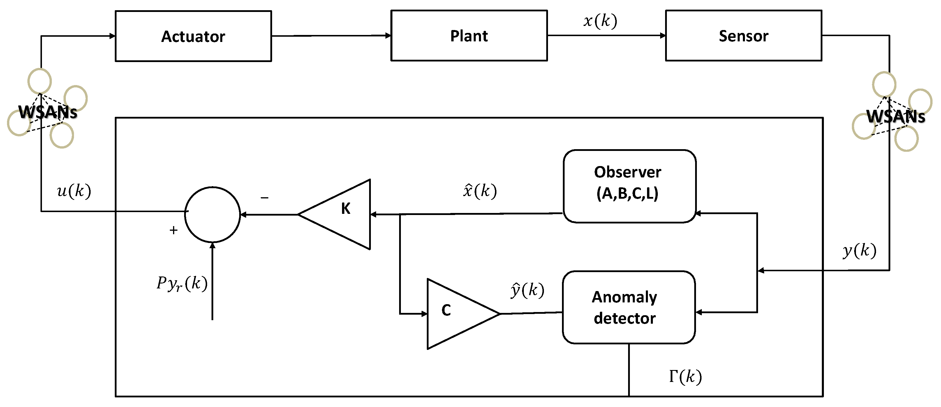
Figure 1 shows the system model of CPSs: a physical system, a computing system, and networks. The physical system includes a sensor and an actuator. First, a clock-driven sensor periodically samples the plant output every . Thereafter, an event-driven controller calculates the actuation commands as soon as the sensor data arrive. The computing system monitors and controls the state of the plant. The observer estimates the state of the physical system and a feedback controller. Generally, event-driven actuators can immediately respond to updated actuation commands.
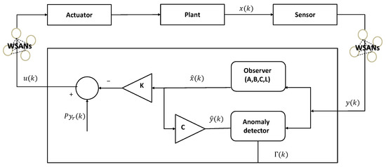
Figure 1.
System model of industrial CPSs.
The physical system is modeled as a linear time-invariant (LTI) single-input single-output system. The computing system consists of an observer, a feedback controller, and an anomaly detector, where each component estimates the state of the physical system, calculates the control input signal, and determines the system anomalies [37]. The physical and computing systems were designed in the discrete-time domain. We consider the dynamics of the physical system as follows:
where is the system matrix containing one or more eigenvalues with magnitudes greater than 1, is the input matrix, is the output matrix, is the state of the physical system, is the control input, and is the sensor output. For the LTI system of (1), we assumed that the pair was controllable, and the pair was observable. The eigenvalues of A, whose magnitude is greater than 1, become the unstable poles of the transfer function form of (1) from u to y.
We consider the observer-based feedback controller on the computing system as follows:
where is the state estimate, is the reference signal, P is a scalar gain, is the state-feedback controller gain, and is the observer gain. We assume that K and L in (2) are appropriately selected to stabilize the system of (1). In other words, they were selected such that both and were Schur matrices. Gain P was selected to satisfy to achieve asymptotic tracking for a constant , where is the n-dimensional unity matrix.
3.2. Wireless Communication System
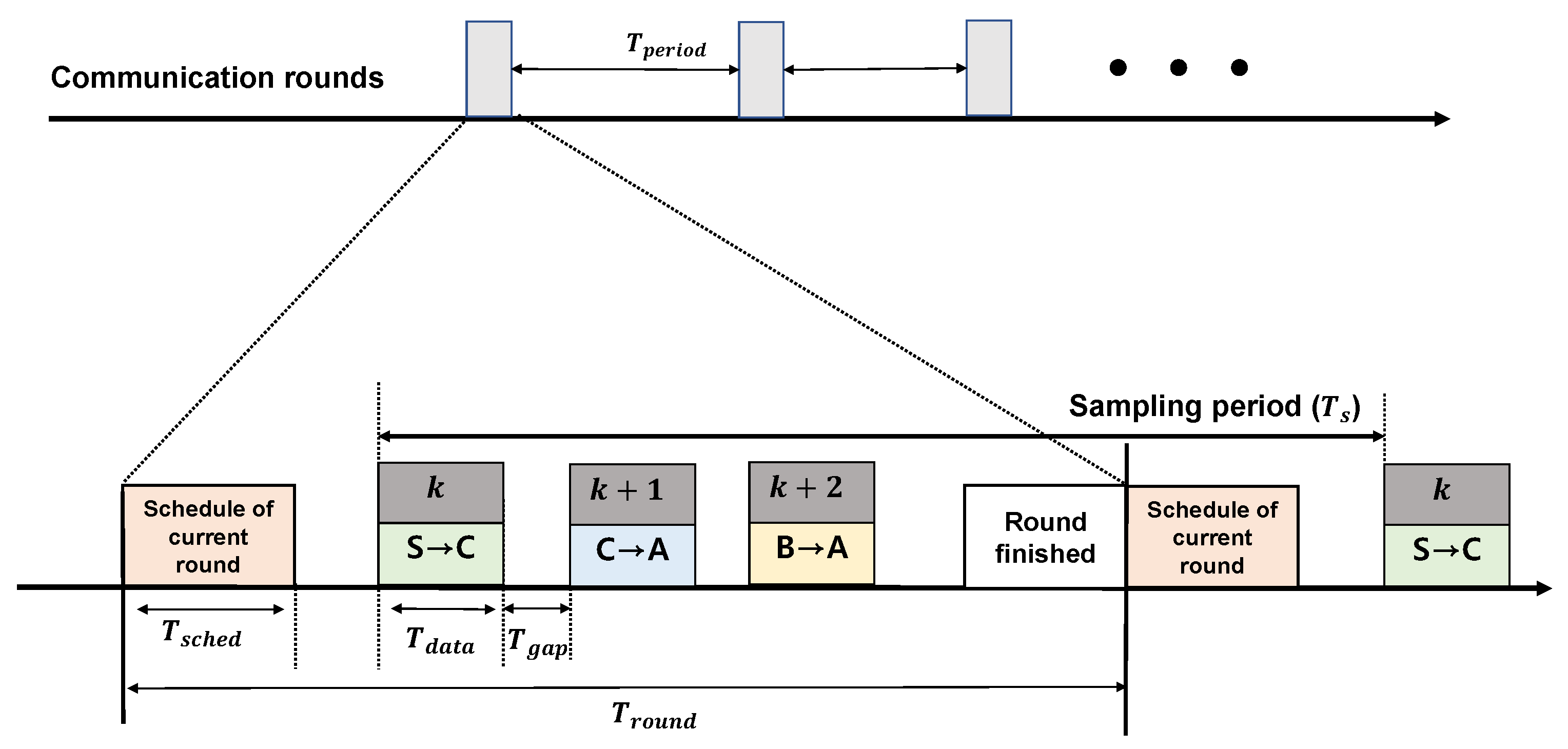
We focus on the LWB protocol for our CPS design because it was designed as a low-power multihop wireless solution. LWB provides a higher-layer protocol and shared-bus application abstraction. This is based on IEEE 802.15.4 radios with O-QPSK modulation in the 2.4 GHz band. The LWB protocol enables reliable communication among sensors, actuator, and controller. In every slot, as shown in Figure 2, one initiator node transmits a message to all the others using a Glossy flood [8]. Since it employs synchronous transmission, it provides reliability above 99.9% in real-world scenarios. The external interference and node failures only marginally affect LWB performance [8]. In addition, LWB is a suitable protocol for controller switching. Unlike WirelessHART’s TDMA, the backup controller can overhear the information between plant and main controller due to the characteristic of flooding communication. In addition, it is unnecessary to consider the independent wireless link status for any time-varying network topology.
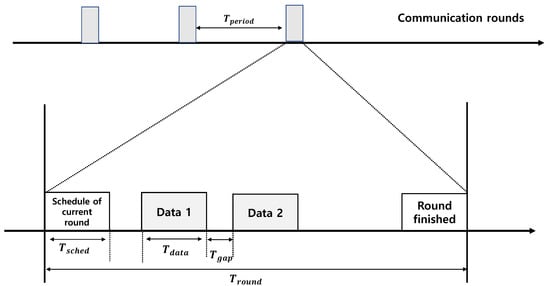
Figure 2.
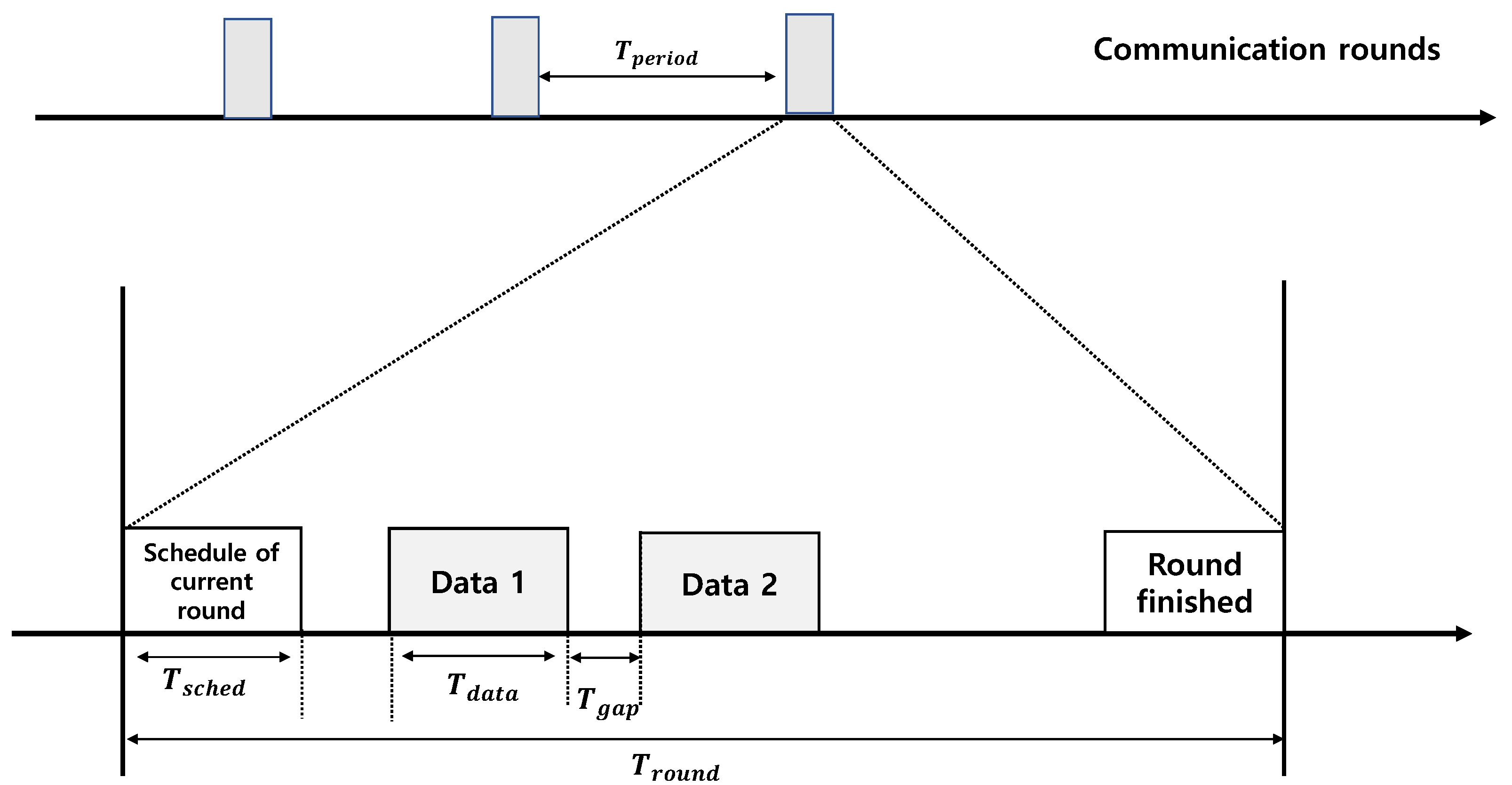
Communication rounds in LWB protocol.
The LWB network consists of a host node and several source nodes. Similar to the network manager in WirelessHART, the host node schedules and manages the source nodes. In every slot, one initiator node transmits a message to all others using a Glossy flood. Glossy [38] exploits the constructive interference of IEEE 802.15.4 symbols for fast network flooding and implicit time synchronization. Glossy affords network flooding and time synchronization. It executes a minimal, deterministic sequence of operations between the packet receptions and retransmissions in order to ensure a constant retransmission delay. Glossy floods are confined to reserved time slots where no other tasks (such as the application or operating system) are allowed to execute. This avoids interference from shared resources, which can cause unpredictable jitter. Consequently, Glossy also enables the nodes to time-synchronize with the initiator.
When a node becomes an initiator and broadcasts a packet, surrounding nodes relay the packet. The receiving side then detects the superposition of multiple signals at the same frequency from multiple transmitters. These synchronous transmissions utilize the constructive interference and the capture effect. The capture effect refers to the phenomenon where a receiver receives one of the synchronously transmitted packets. However, to achieve this effect, the following two conditions must be met:
- 1
- The difference between the receiving power of one signal and the others, and noise is greater than the capture threshold.
- 2
- A weak signal arrives first and a strong signal arrives thereafter; the strong signal can be received if it arrives within the capture window. Because the receiver no longer performs a preamble search upon receipt, it can receive the strong signal if it arrives before the complete preamble.
Both capture threshold and capture window depend on the physical layer. In the case of IEEE 802.15.4, the capture threshold was reported to be 2–3 dB [39], and the capture window was 128 s [40].
Another characteristic is constructive interference, which implies that signals overlap perfectly without time or phase offsets. However, the phase offset varies during reception, although the transmitter can compensate for different path delays owing to the different carrier offsets caused by the asynchronous operation of the transmitter’s radio oscillator. Under IEEE 802.15.4, the oscillators are allowed to drift by ppm, which translates to a maximal frequency offset of 192 kHz between sender and receiver over a 2.4 GHz band [41]. Owing to the carrier frequency offset, there are alternating periods of constructive and destructive interference. Destructive interference can cause bit errors at the receiver. However, a receiver can still successfully receive an entire packet if the signal’s time offset is less than 0.5 s [39]. Thus, the carrier frequency offset is resolved using receiver implementation or an error-correction mechanism. Therefore, the LWB provides a higher-layer protocol and shared-bus application abstraction. In every slot, one initiator node transmits a message to all the others using a Glossy flood [8].
Figure 2 presents an illustration of each round and slot structure in the LWB. Each round consists of a slot for the current round schedule, n data slots, and round finish slots. All nodes repeat each round at every time period, and time for the round is . Each round begins with the schedule of the host, . In this slot, the host node computes the scheduling for the network and broadcasts it to the source nodes. Upon receipt of the scheduling information, one source node becomes the initiator in the allocated slot and launches the Glossy flooding communication. One-hop nodes within the initiator’s transmission range simultaneously receive the transmission and relay all packets simultaneously after the precise processing period. Repeated flooding enables nodes greater than two hops to receive packets sent by the initiator. In a multihop network, the LWB provides reliability exceeding 99.9% under real-world scenarios [8]. Additionally, nodes do not maintain any network state, making the LWB highly robust to network dynamics that result from misbehaving or failing nodes and wireless interference.
To implement the constructive interference of Glossy flooding, wireless signals must be overlapped and synchronized. Therefore, application software executions on communication nodes should be minimized for strict time synchronization. Wireless signal receptions can also fail due to inherent wireless channel uncertainty and interference by other wireless communications. For network failures, Glossy flooding supports packet retransmission, which enhances the reliability of wireless communications.
3.3. Network Scheduling for Control System
We designed the WSAN scheduling without considering switching controllers. Figure 2 presents an illustration of each round and slot structure in the LWB. Each round consists of a slot for the current round schedule, n data slots, and round finish slots. All nodes repeat each round at every time period, and the time for the round is . Each round begins with the schedule of the host, . In this slot, the host node computes the scheduling for the network and broadcasts it to the source nodes. Upon receipt of the scheduling information, one source node becomes the initiator in the allocated slot and launches the Glossy flooding communication. One-hop nodes within the initiator’s transmission range simultaneously receive the transmission and relay all packets simultaneously after the precise processing period. Repeated flooding enables nodes greater than two hops to receive packets sent by the initiator.
The transmission of sensor and actuator information should be assigned to each round’s data slot, considering the sampling period of the control system. First, it was necessary to examine the composition of each round, which was repeated every . Additionally, there were multiple slots in each round. Each slot was assigned to each source node that initiated the Glossy transmission, and various parameters determined its length.
The reliability of packet reception improved with the repetition of transmission in the slot. If the transmission was repeated N times, the reliability of packet reception increased. However, N iterations were required for nodes away from the initiator to receive packets, requiring a sufficiently long slot time, which can be calculated as follows:
where H is the maximal number of hops in the network, and is the time for one-hop transmission.
is a function of the length of packet L, and if the bitrate is 250 kbps, the value is constant. The transmission overhead is 300 s per hop, which includes the transmission of four preamble bytes and the sync word (4 B). Length of a round depends on the physical systems and the control systems in the WSANs, with a trade-off between a higher energy overhead per round and the possibility of supporting shorter periods and deadlines. Within one round, there are multiple data slots and two for scheduling. There exists a time gap between the slots. During this gap time, the transmitted packets are placed into the incoming packet queue, and the received payloads are processed. The length of a round is calculated as
where is the number of assigned slots. We used one slot for the transmission of sensor information and another slot for the transmission of actuator information in the WSANs using LWB. These two slots were repeated in cycles of sampling period . Depending on , there are various methods to set up a round. First, can be set as long as possible, such that two slots are repeated many times within . The second method only uses two slots for communication during the round, which is achieved by setting to be the same as . The battery performance of the system may vary depending on how the round is set. An excessively short round can cause problems in terms of battery efficiency owing to the frequent rescheduling calculations and transmissions, although there are no changes in the network. However, it is necessary to set appropriately because, if a round is excessively long, it becomes difficult to cope with changes in the network. In this study, was set to be the same as the sampling interval of the control system in order to explore its stability in terms of dynamic channel environments.
4. Controller Switching Mechanism
In this section, we present a codesign approach for the switching controllers. The process of the proposed controller switching mechanism is illustrated in Figure 3. The proposed mechanism detects controller failures combined with a backup controller to maintain stability in case of a primary controller is failed. First, a plant is controlled through the primary controller as shown Figure 3a. The sensor information of the plant is delivered to the primary controller, and the primary controller generates control information and transmits it to the plant. A host node in WSANs generates network scheduling information and passes it to each node in the network. The backup controller frequently checks the primary controller for failures by monitoring the communication status between the plant and the primary controller. As shown in Figure 3b, the backup controller detects failures in the current controller and replaces the current controller in the case of an emergency. In this controller switching mechanism, the primary and backup controllers have the same hardware and control functions to calculate control input signals for plant actuation, where roles of these controllers can be determined by a CPS administrator. The only difference between primary and backup controller is that the backup controller has a fault-checking function of the primary controller. Furthermore, we assumed that the backup controller was reliable and would not break down.
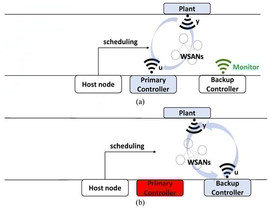
Figure 3.
Process of proposed controller switching mechanism (a) before and (b) after controller switching.
To ensure the stability of the control system, we designed the controller switching to occur under the maximal allowable delay bound (MADB) conditions. In this section, we analyze the LWB network delay and MADB. Then, we designed the WSAN scheduling of the LWB protocol and algorithm for switching controller, so that the delay did not exceed MADB conditions.
4.1. LWB Network Delay
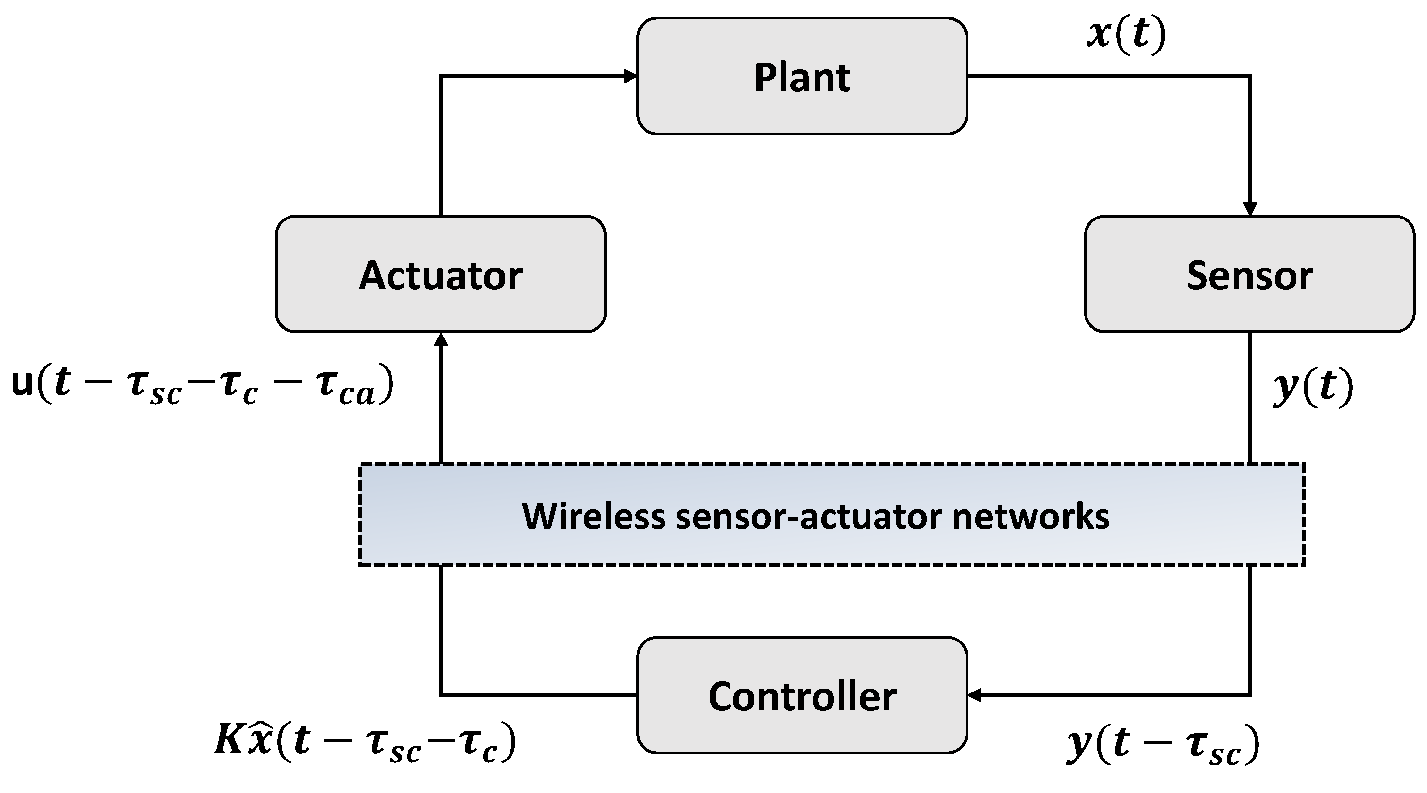
In WSANs, network delays significantly affect the performance and stability of the control system. A network delay in the scheduling technique considering LWB controller switching was analyzed, and delay analysis in the discrete domain was conducted. As shown in Figure 4, the delay mainly comprised the delay from the sensor to the controller, , and that from the controller to the actuator, .
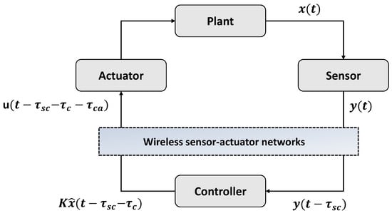
Figure 4.
Network delay in WSANs.
and comprise a queuing delay, a frame delay, and a propagation delay, and values that vary depend on the protocol’s design of the protocol. Additionally, a computation delay occurs in controller ; typically, such delays are very small compared with communication delays, and can thus be neglected. Thus, the total delay is . If a controller fails or packet dropout occurs, the time delay is , where d is the number of dropouts. The time delay should be less than the MADB to ensure the stability of the control system. Delays in LWB networks are bounded and constant because data transmission is achieved within a predefined time interval. and comprise a given amount of time required to process the data received from the controller and the plant and to generate the data to be transmitted. In the proposed design, data are processed at .
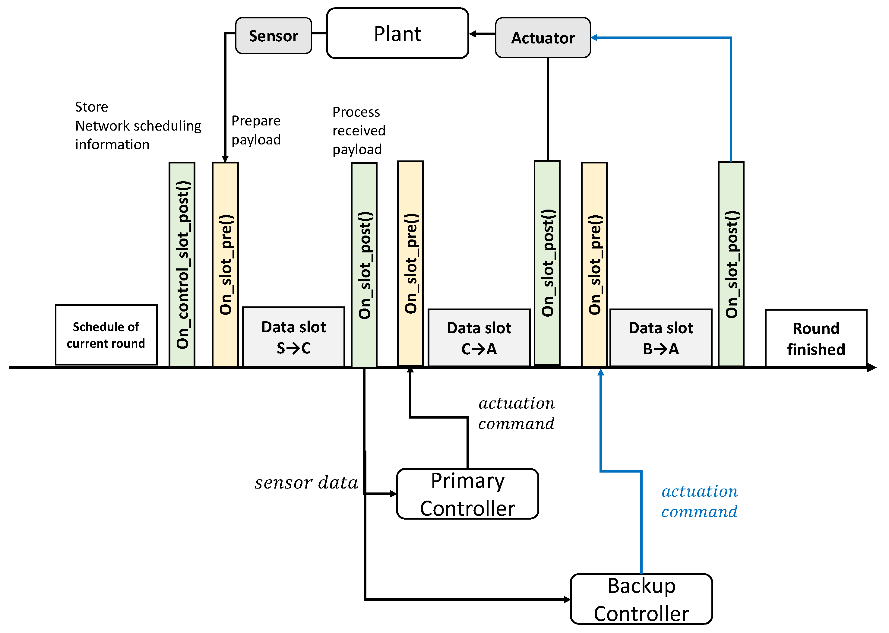
Figure 5 illustrates details of the controller switching mechanism. As shown in Figure 5, and callback functions were executed between the two data slots, for preparing the payload and process the received payload. The repetition of transmission occur at . and is in LWB networks. Therefore, the total delay in the LWB becomes . For instance, if the controller does not function, a switch to the backup controller occurs in the current round, and the total delay becomes .

Figure 5.
Implementation detail of scheduling with controller switching.
4.2. MADB
The MADB is the maximal sampling period that guarantees stability even with low system performance. Numerous methods have been developed to analyze the stability of network control systems. Most of these methods employ Lyapunov stability analysis and provide conditions for the global asymptotic stability of a system [42] Furthermore, a majority of the reported methods are typically overcomplicated for practical applications. By contrast, a simple stability analysis method was presented in [43] that allowed the determination of the MADB in a continuous network control system derived using the finite difference approximation of the delay term and the Lyapunov system stability theorem. More detailed proofs and details can be found in [43]. We considered a continuous state-space representation that is given by
where , and are system state vector, system control input, and system output, respectively. Furthermore, and D are the constant matrices with appropriate size. The state feedback controller is expressed as
where K is feedback controller gain matrix. The following were assumed:
- 1
- Time-driven sensor and event-driven actuator transmit data as a single packet and reject old packets.
- 2
- All system states are measurable and ready to be sent. The time delay is sufficiently small to be less than 1 unit of measurement.
Theorem 1.
Considering that the above-mentioned assumptions hold, for the system of (6) with the feedback control of (7), the closed-loop system is globally asymptotically stable if , for i = 1, 2, … , n and all the second-order reminders of the state variables are sufficiently small for the given value of τ, where Ψ is given by
Here, are the eigenvalues of Ψ that must lie on the left-hand side of the complex plane. The second-order reminders refer to Taylor series expansion of state variables .
Corollary 1.
Corollary 2.
4.3. Network Scheduling with Controller Switching
Here, we discuss network scheduling for controller switching algorithms. In the scheduling algorithm for controller switching, the only difference compared to scheduling without switching is the addition of a slot to transmit to the backup controller. This slot is only allocated, and transmission does not occur if the controller operates appropriately. The slot assignment for the switching algorithm is illustrated in Figure 6. The backup controller can receive sensor information from the plant by using a previously assigned slot for the controller (slot k). Unlike WirelessHART’s TDMA, the LWB can receive sensor information from the plant, although the distance between the controller and backup controller is large. The backup controller monitors communications between the controller and the plants to detect controller misbehavior. In the event of an anomaly, the backup controller operates on behalf of the original controller, and the backup controller also notifies the host node so that the network can be reorganized.

Figure 6.
Network scheduling with controller switching. C, primary controller; S, sensor in a plant; A, actuator in a plant; and B, backup controller.
We used the MADB as the timeout threshold to identify anomalies of the controller. If the backup controller does not receive an actuation command from the primary controller within a timeout threshold, the backup controller takes over. The pseudocode of the switching algorithm is presented in Algorithm 1. The backup controller increases the count value by 1 if it does not receive a packet from the primary controller’s action command in the slot. In this study, was set to be the same as the sampling interval of the control system. Therefore, if the count value and product are less than the MADB, the backup controller skips this round. The stability of the control system can be ensured by transmitting the slot assigned to the next round. However, if the count value and product are greater than the MADB, the backup controller must transmit on behalf of the primary controller to ensure the stability of the control system. Lastly, when a back-controller transfer occurs, it is passed via piggyback to the host node. The host node then notifies the administrator regarding the failure of the controller.
| Algorithm 1 Pseudocode of switching algorithm in backup controller |
|
5. Performance Evaluation
We conducted network experiments before connecting the control system. TelosB motes were used to build wireless sensor–actuator networks. TelosB is a 2.4 GHz IEEE 802.15.4 Chipcon wireless transceiver with a data rate of 250 kbps. Baloo, based on Contiki-NG, was used to program the motes. Contiki-NG is an operating system used for resource-constrained devices on the Internet of Things. Baloo [11] is a framework for network stacks based on synchronous transmissions.
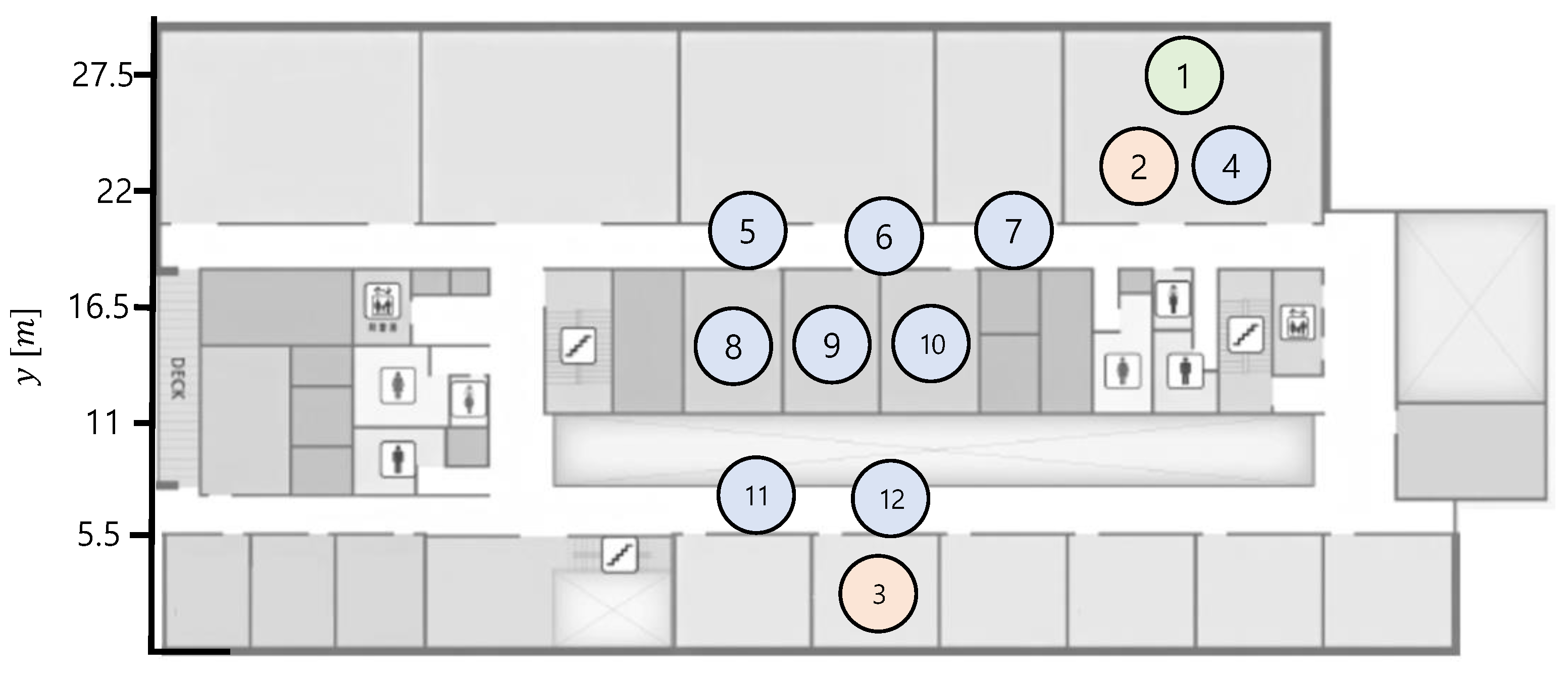
Figure 7 shows a testbed used in WSANs experiments. It is a floor plan in which the network nodes are arranged, where the distance between a transmitter (node-3) and receiver is 30 m. The TelosB motes have indoor transmission coverage of 20–30 m, which can be diminished by signal attenuation from the walls on the building. However, the distance between each node is less than 10 m. Therefore, in the experiments, we do not consider transmission failures by the physical signal attenuation or obstacles. Furthermore, to minimize the interference by other wireless communications, such as WiFi communications by smartphones, we conduct the experiments at night time.
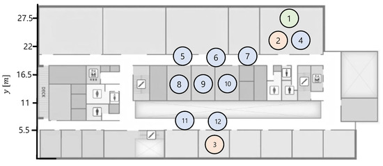
Figure 7.
Testbed used in network experiments. Red and blue circles are transmitter nodes and relay nodes, respectively. Green circle denotes a receiver node.
Red circles in Figure 7 are the transmitter nodes that transmit packets to a receiver node (green circles). Initially, node-2 transmits packets to node-1. Thereafter, we cut off the power of node-2 and checked whether node-3 could start transmission on behalf of node-2. For node-3 to perform the switching algorithm, it must be possible to receive packets transmitted by node-2 to node-1.
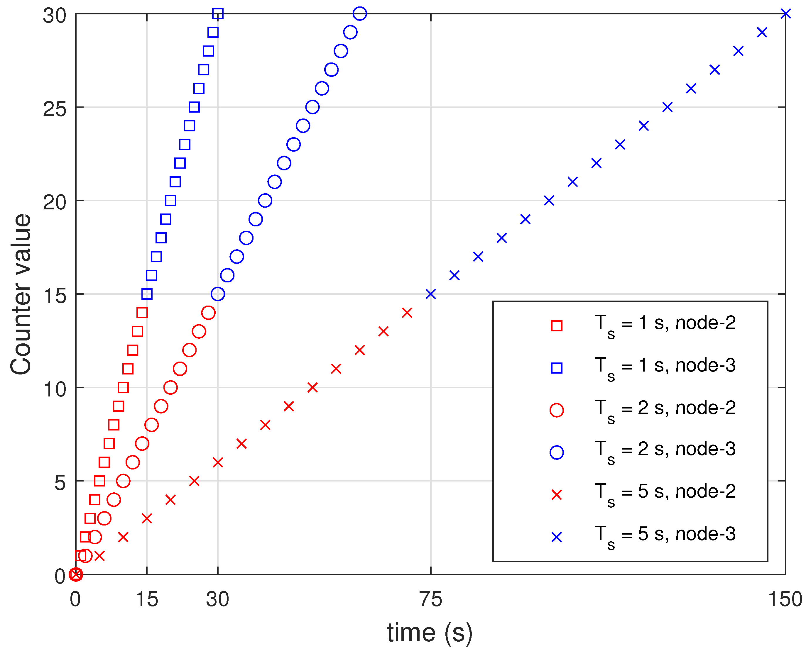
Node-2 was programmed to transmit 2 B data, including its own node number (1 B) and counter value (1 B), to the host node. The counter value increased by 1 every round. We stopped the operation of node-2 when the counter value reaches 15 and checked whether node-3 was working properly. We checked if switching could take place in the current round. Figure 8 presents the performance of the proposed switching algorithm by changing to 1, 2, and 5 s. We conducted the experiment 10 times for each . When the transmission of node-2 (red marker) was stopped, node-3 started transmission (blue marker) as shown in Figure 8. Results indicate that the proposed network scheduling and algorithm for switching can be applied for control systems.
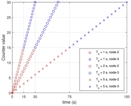
Figure 8.
Performance of switching algorithm in WSAN testbed experiments.
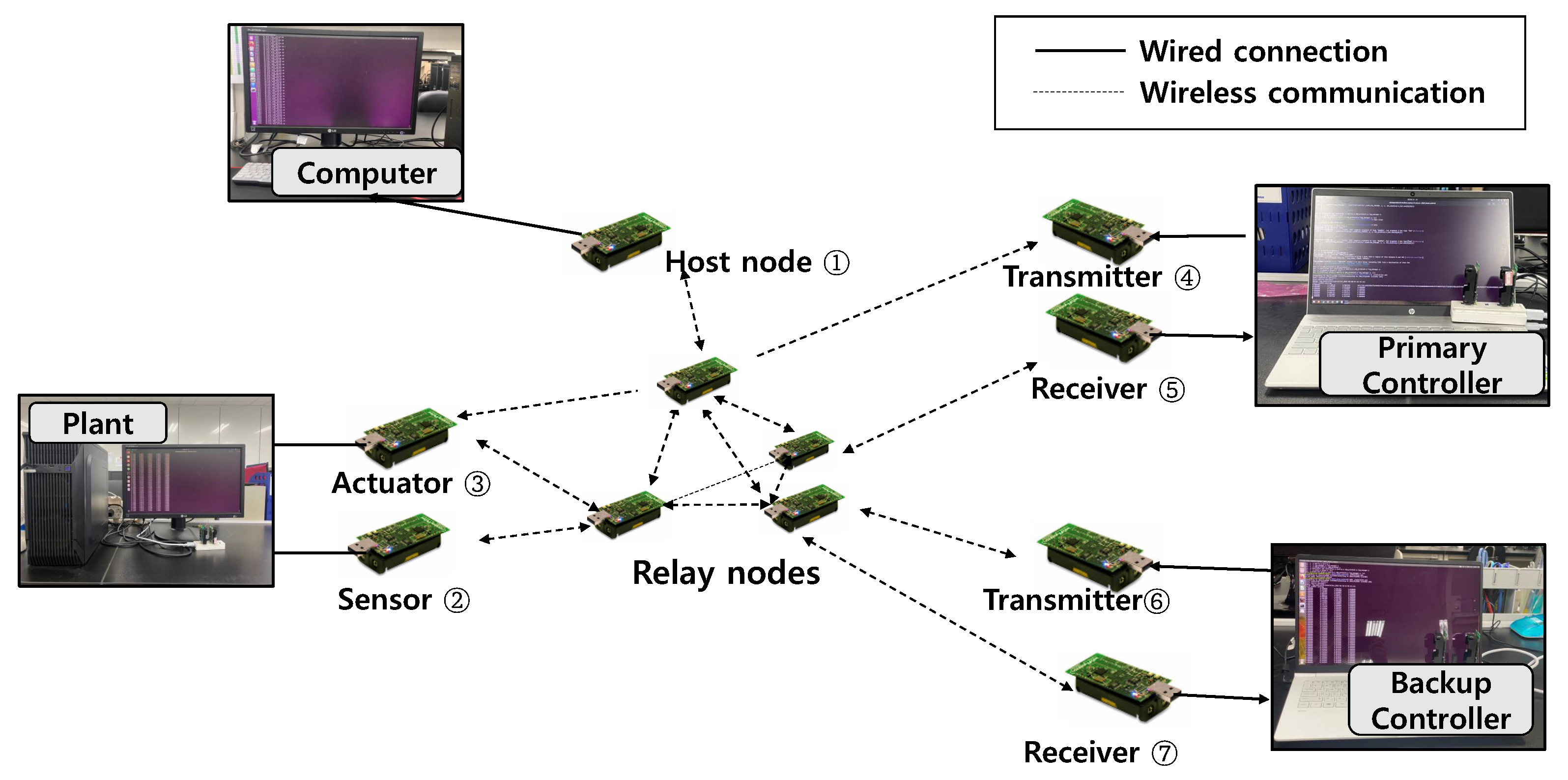
Next, we evaluated performance by using a hardware-in-the-loop experiment for controller switching. We established a testbed that combined a physical wireless network with a simulated model of a control system to create a hardware-in-the-loop experiment. Figure 9 shows the experimental configuration. The testbed consisted of TelosB motes and computers. All motes participated in Glossy flooding communication as a node. We programmed node-1 as a host node to compute the network scheduling for the network and broadcasts it to the source nodes.
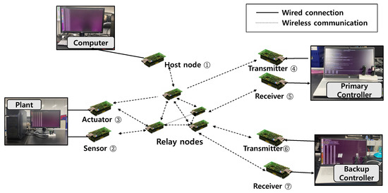
Figure 9.
Experimental configuration.
We used a total of four computers for the experiment. While communications between motes were wireless, wired communications were used to connect computers and motes. We connected the computers and the motes using a built-in USB port of motes. To monitor the network situation, we connected the host node to one computer and set the host node to transmit status information of network periodically. The remaining three computers were used for the simulation of a control system. Each simulated a primary controller, a backup controller, and a plant. The plant received actuator state changes from node-3 and produced sensor readings as output. The sensor nodes received values from the computer instead of a real sensor and sent it to the controllers.
The controller also consisted of a transmitter node and a receiver node. Here, two nodes were used to reduce the delay caused by USB serial communications. In [26], an additional piece of equipment called Bolt was used to reduce computation delays. To reduce delays instead of using additional equipment, we employed two nodes for separately receiving and transmitting radio communications. The receiver node was only used to send the received data from network to computer, whereas the radio transmission node was used to receive data from the computer. This configuration reduced the computation delay between computers and motes at a low cost in a general-purpose control system. Apart from the relay node, five nodes were required by default, and two more were required for the backup controller.
To implement the controller design, considering the design and switching ideas described earlier, the program flow of Baloo is as follows. The host checks for updated control information and prepares and sends the control packet. The regular nodes receive these control packets. A node transitions to the running state after it receives a valid control packet in on callback. For each data slot, if the sensor node is the initiator, the slot is assigned to the sensor nodes. and is set to 8 ms and 16 ms, respectively. We used Baloo’s preinstalled functions to serially communicate with the computers. We employed the and callback functions that were executed between the two data slots, , as shown in Figure 5. The original purpose of the is to pass the payload ahead of each data slot. We used the -callback function to read the sensor data and actuator commands from the computer. If the controller’s receiver nodes or actuator nodes receive sensor or actuator data in a data slot, the nodes execute the callback function to process the received payload. We used the callback function to serially send the received payload to the computer.
The controller switching mechanism also employed two callback functions. As shown in Figure 5, the backup controller can also read sensor data in the after the slot for sending sensor data to controller owing to the LWB characteristics. Following the data slot used to send the actuation command from the controller, the backup controller runs Algorithm 1 for controller switching in order to monitor the controller’s fault. If the backup controller decides to send an actuation command, it prepares the payload to send in prior to the data slot for the backup controller.
With regard to the packet structure, sensor and actuator information is transmitted up to six decimal places. To reduce the size of the payload, we sent unsigned char data by two digits in the case of decimal places. Additionally, 1 B was used as an indicator for classifying the sensor and actuation data. The signs of the data and node identifier were included in the payload; each was 1 B. The total size of the payload was 8 B. The Glossy header was 2 B for Glossy, with a content-redundancy check of 16 bits. Therefore, the total packet size was 12 B.
The control execution time based on applying traditional implementation guidelines varies significantly depending on process type. The computer simulations were developed in consideration of processes such as temperature, composition, and level control that require 8 or 16 s wireless communication update rate. In the experiments, we installed the plant simulator and feedback controller simulator software proposed in [37], where the plant and controller software was installed in the plant computer and two controller computers, respectively. The plant software updates state of the plant with linear dynamics (1), and actuates state with control input signal received from the controller software. In every sampling period , the plant software generates sensor output packets with state and output matrix C in the dynamics (1); then, it transmits the sensor output packets to controller computers. The plant model embedded in the plant software is defined in (1) with the following parameters:
where sampling period is 2 s.
The controller software embedded in the controller computers conducts observer-based feedback control, which estimates the state of the plant with the sensor output packets, and calculates control input signals as illustrated in the control logic (2). Then, the controller software generates the control input signal packets, and transmits them to the plant computer. The parameters of the observer-based state feedback controller in (2) were chosen as follows:
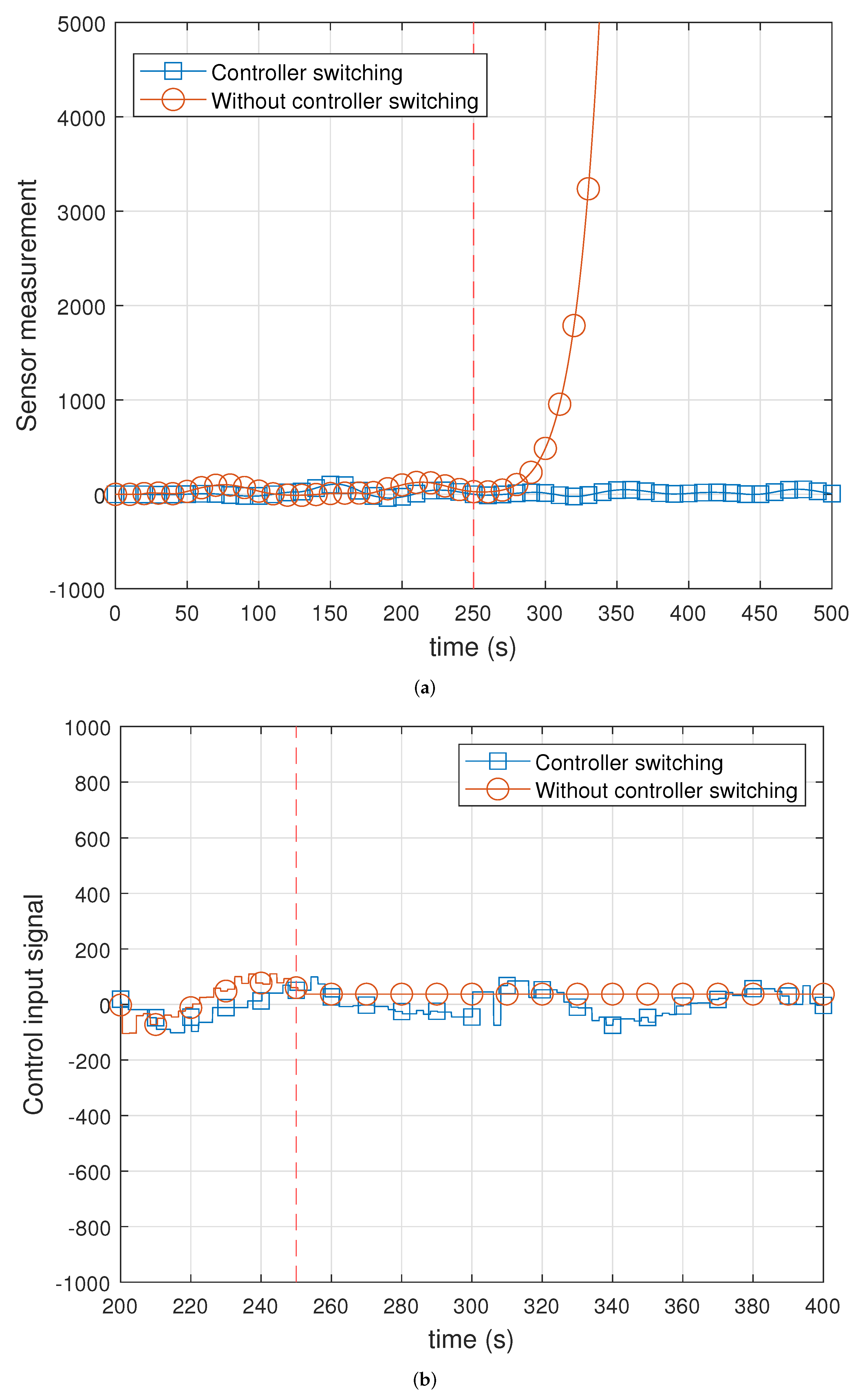
Figure 10 shows the result of using the switching mechanism. We stopped the primary controller simulator at 250 s to check the controller switching mechanism (vertical line with a constant 250 value). We displayed a marker every 10 s. Figure 10b shows the results of the sensor measurements. The backup controller detected malfunctions in the controller and initiated transmission in place of the controller. However, the state of the plant increased to infinity without a controller switching mechanism after 250 s. Figure 10b shows the result of the control input signals. Unlike when the switching mechanism was used, the primary controller could no longer transmit the control input signal. Therefore, the plant performed control by using the control input value transmitted at 250 s as it is. Results indicate that the proposed mechanism could quickly recover by switching to the backup controller in the case of controller failure.
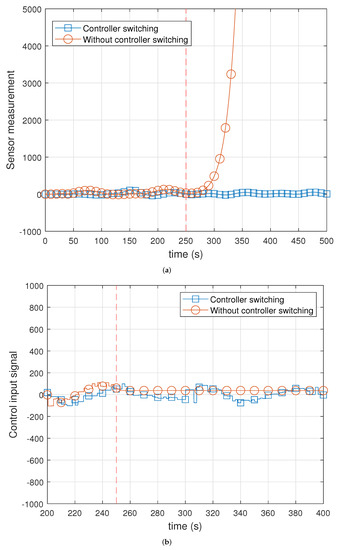
Figure 10.
Experimental results on plant with/without controller switching mechanism. (a) Sensor measurements; (b) control input signals.
6. Conclusions
We proposed a new WSAN capable of enhancing control system resiliency. A controller switching mechanism was introduced to ensure resilience against problems, such as controller failures in the controller network. MADB-based time-outs were used for fault detection, and the LWB protocol was used to provide broadcast communications. The backup controller receives the sensor information from the physical system; as it uses a synchronous transmission, it is not necessary to consider the independent wireless link status for time-varying network, which enables fast switching. For verification, an experiment was conducted by serially connecting a TelosB mote to a computer. Results indicated that the proposed mechanism could quickly recover by switching to the backup controller in the case of controller failure. As future work, we will extend the controller switching mechanism to guarantee the safety of physical systems under cyber–physical attacks. One possibility is to investigate a physical-knowledge-based anomaly detector to detect cyberattacks.
Author Contributions
Conceptualization, B.-M.C. and K.-J.P.; methodology, investigation, B.-M.C. and S.K.; simulation and validation, B.-M.C. and S.K.; writing—original draft preparation, B.-M.C.; writing—review and editing, K.-D.K. and K.-J.P.; visualization, B.-M.C.; supervision, K.-J.P.; project administration, K.-J.P.; funding acquisition, K.-J.P. All authors have read and agreed to the published version of the manuscript.
Funding
This work was partly supported by an Institute for Information and Communications Technology Promotion (IITP) grant funded by the Korean government (MSIP) (2021-0-01277, development of attack response and intelligent RSU technology for vehicle security threat prevention) and a National Research Foundation of Korea (NRF) grant funded by the Korean government (MSIT) (NRF-2019R1A2C1088092).
Conflicts of Interest
The authors declare no conflict of interest.
References
- Kim, K.D.; Kumar, P.R. Cyber-physical systems: A perspective at the centennial. Proc. IEEE 2012, 100, 1287–1308. [Google Scholar]
- Park, K.J.; Zheng, R.; Liu, X. Cyber-physical systems: Milestones and research challenges. Comput. Commun. 2012, 36, 1–7. [Google Scholar] [CrossRef]
- Javaid, N. Integration of context awareness in Internet of Agricultural Things. ICT Express 2021. (Early Access). [Google Scholar] [CrossRef]
- Li, J.Q.; Yu, F.R.; Deng, G.; Luo, C.; Ming, Z.; Yan, Q. Industrial internet: A survey on the enabling technologies, applications, and challenges. IEEE Commun. Surv. Tutor. 2017, 19, 1504–1526. [Google Scholar] [CrossRef]
- Park, P.; Ergen, S.C.; Fischione, C.; Lu, C.; Johansson, K.H. Wireless network design for control systems: A survey. IEEE Commun. Surv. Tutor. 2017, 20, 978–1013. [Google Scholar] [CrossRef]
- Zhang, L.; Chen, X.; Kong, F.; Cardenas, A.A. Real-Time Attack-Recovery for Cyber-Physical Systems Using Linear Approximations. In Proceedings of the 2020 IEEE Real-Time Systems Symposium (RTSS), Houston, TX, USA, 1–4 December 2020; pp. 205–217. [Google Scholar]
- Paridari, K.; O’Mahony, N.; Mady, A.E.D.; Chabukswar, R.; Boubekeur, M.; Sandberg, H. A framework for attack-resilient industrial control systems: Attack detection and controller reconfiguration. Proc. IEEE 2017, 106, 113–128. [Google Scholar] [CrossRef]
- Ferrari, F.; Zimmerling, M.; Mottola, L.; Thiele, L. Low-power wireless bus. In Proceedings of the 10th ACM Conference on Embedded Network Sensor Systems, Toronto, ON, Canada, 6–9 November 2012; pp. 1–14. [Google Scholar]
- Jurado Pérez, L.; Salvachúa, J. Simulation of Scalability in Cloud-Based IoT Reactive Systems Leveraged on a WSAN Simulator and Cloud Computing Technologies. Appl. Sci. 2021, 11, 1804. [Google Scholar] [CrossRef]
- Willow. TelosB Datasheet. 2008. Available online: https://www.willow.co.uk/TelosB_Datasheet.pdf (accessed on 9 July 2021).
- Jacob, R.; Bächli, J.; Da Forno, R.; Thiele, L. Synchronous Transmissions made easy: Design your network stack with Baloo. In Proceedings of the 2019 International Conference on Embedded Wireless Systems and Networks (EWSN’19), Beijing, China, 25–27 February 2019; pp. 106–117. [Google Scholar]
- Blevins, T.; Chen, D.; Nixon, M.; Wojsznis, W. Wireless Control Foundation: Continuous and Discrete Control for the Process Industry; International Society of Automation Triangle Park: Durham, NC, USA, 2015; Volume 4. [Google Scholar]
- De Carvalho Silva, J.; Rodrigues, J.J.; Alberti, A.M.; Solic, P.; Aquino, A.L. LoRaWAN—A low power WAN protocol for Internet of Things: A review and opportunities. In Proceedings of the 2017 2nd International Multidisciplinary Conference on Computer and Energy Science (SpliTech), Split, Croatia, 12–14 July 2017; pp. 1–6. [Google Scholar]
- Mekki, K.; Bajic, E.; Chaxel, F.; Meyer, F. A comparative study of LPWAN technologies for large-scale IoT deployment. ICT Express 2019, 5, 1–7. [Google Scholar] [CrossRef]
- Ramirez, R.; Huang, C.Y.; Liao, C.A.; Lin, P.T.; Lin, H.W.; Liang, S.H. A Practice of BLE RSSI Measurement for Indoor Positioning. Sensors 2021, 21, 5181. [Google Scholar] [CrossRef]
- Demirkol, I.; Ersoy, C.; Alagoz, F. MAC protocols for wireless sensor networks: A survey. IEEE Commun. Mag. 2006, 44, 115–121. [Google Scholar] [CrossRef]
- De Guglielmo, D.; Brienza, S.; Anastasi, G. IEEE 802.15. 4e: A survey. Comput. Commun. 2016, 88, 1–24. [Google Scholar] [CrossRef]
- Ayoub, W.; Samhat, A.E.; Nouvel, F.; Mroue, M.; Prévotet, J.C. Internet of mobile things: Overview of LoRaWAN, DASH7, and NB-IoT in LPWANs standards and supported mobility. IEEE Commun. Surv. Tutor. 2019, 21, 1561–1581. [Google Scholar] [CrossRef] [Green Version]
- Jeon, K.E.; She, J.; Soonsawad, P.; Ng, P.C. BLE beacons for internet of things applications: Survey, challenges, and opportunities. IEEE Internet Things J. 2018, 5, 811–828. [Google Scholar] [CrossRef]
- Raza, M.; Aslam, N.; Le-Minh, H.; Hussain, S.; Cao, Y.; Khan, N.M. A critical analysis of research potential, challenges, and future directives in industrial wireless sensor networks. IEEE Commun. Surv. Tutor. 2018, 20, 39–95. [Google Scholar] [CrossRef]
- Salarian, H.; Chin, K.W.; Naghdy, F. Coordination in wireless sensor-actuator networks: A survey. J. Parallel Distrib. Comput. 2012, 72, 856–867. [Google Scholar] [CrossRef]
- Wu, C.; Gunatilaka, D.; Sha, M.; Lu, C. Real-time wireless routing for industrial internet of things. In Proceedings of the 2018 IEEE/ACM Third International Conference on Internet-of-Things Design and Implementation (IoTDI), Orlando, FL, USA, 17–20 April 2018; pp. 261–266. [Google Scholar]
- Gunatilaka, D.; Lu, C. Conservative channel reuse in real-time industrial wireless sensor-actuator networks. In Proceedings of the 2018 IEEE 38th International Conference on Distributed Computing Systems (ICDCS), Vienna, Austria, 2–6 July 2018; pp. 344–353. [Google Scholar]
- Park, P.; Di Marco, P.; Johansson, K.H. Cross-layer optimization for industrial control applications using wireless sensor and actuator mesh networks. IEEE Trans. Ind. Electron. 2016, 64, 3250–3259. [Google Scholar] [CrossRef]
- Stanoev, A.; Aijaz, A.; Portelli, A.; Baddeley, M. Closed-Loop Control over Wireless–Remotely Balancing an Inverted Pendulum on Wheels. arXiv 2020, arXiv:2003.10571. [Google Scholar]
- Mager, F.; Baumann, D.; Jacob, R.; Thiele, L.; Trimpe, S.; Zimmerling, M. Feedback control goes wireless: Guaranteed stability over low-power multi-hop networks. In Proceedings of the 10th ACM/IEEE International Conference on Cyber-Physical Systems, Montreal, QC, Canada, 16–18 April 2019; pp. 97–108. [Google Scholar]
- Ma, Y.; Lu, C. Efficient holistic control over industrial wireless sensor-actuator networks. In Proceedings of the 2018 IEEE International Conference on Industrial Internet (ICII), Seattle, WA, USA, 231–23 October 2018; pp. 89–98. [Google Scholar]
- Baumann, D.; Mager, F.; Zimmerling, M.; Trimpe, S. Control-guided communication: Efficient resource arbitration and allocation in multi-hop wireless control systems. IEEE Control. Syst. Lett. 2019, 4, 127–132. [Google Scholar] [CrossRef] [Green Version]
- Priya, N.; Pankajavalli, P. Review and future directions of Fault Tolerance schemes and applied techniques in Wireless Sensor Networks. Int. J. Comput. Sci. Eng. 2019, 7, 599–606. [Google Scholar] [CrossRef]
- Yarinezhad, R.; Hashemi, S.N. Distributed faulty node detection and recovery scheme for wireless sensor networks using cellular learning automata. Wirel. Netw. 2019, 25, 2901–2917. [Google Scholar] [CrossRef]
- Zhu, J.; Yu, H.; Lin, Z.; Liu, N.; Sun, H.; Liu, M. Efficient actuator failure avoidance mobile charging for wireless sensor and actuator networks. IEEE Access 2019, 7, 104197–104209. [Google Scholar] [CrossRef]
- Bak, S.; Chivukula, D.K.; Adekunle, O.; Sun, M.; Caccamo, M.; Sha, L. The system-level simplex architecture for improved real-time embedded system safety. In Proceedings of the 2009 15th IEEE Real-Time and Embedded Technology and Applications Symposium, San Francisco, CA, USA, 13–16 April 2009; pp. 99–107. [Google Scholar]
- Keliris, A.; Salehghaffari, H.; Cairl, B.; Krishnamurthy, P.; Maniatakos, M.; Khorrami, F. Machine learning-based defense against process-aware attacks on industrial control systems. In Proceedings of the 2016 IEEE International Test Conference (ITC), Fort Worth, TX, USA, 15–17 November 2016; pp. 1–10. [Google Scholar]
- Yoon, S.; Lee, J.; Kim, Y.; Kim, S.; Lim, H. Fast controller switching for fault-tolerant cyber-physical systems on software-defined networks. In Proceedings of the 2017 IEEE 22nd Pacific Rim International Symposium on Dependable Computing (PRDC), Christchurch, New Zealand, 22–25 January 2017; pp. 211–212. [Google Scholar]
- Kim, S.; Won, Y.; Park, I.H.; Eun, Y.; Park, K.J. Cyber-physical vulnerability analysis of communication-based train control. IEEE Internet Things J. 2019, 6, 6353–6362. [Google Scholar] [CrossRef]
- Ma, Y.; Lu, C.; Sinopoli, B.; Zeng, S. Exploring Edge Computing for Multitier Industrial Control. IEEE Trans. Comput. Aided Des. Integr. Circuits Syst. 2020, 39, 3506–3518. [Google Scholar] [CrossRef]
- Kim, S.; Eun, Y.; Park, K.J. Stealthy sensor attack detection and real-time performance recovery for resilient CPS. IEEE Trans. Ind. Inform. 2021, 17, 7412–7422. [Google Scholar] [CrossRef]
- Ferrari, F.; Zimmerling, M.; Thiele, L.; Saukh, O. Efficient network flooding and time synchronization with glossy. In Proceedings of the 10th ACM/IEEE International Conference on Information Processing in Sensor Networks, Chicago, IL, USA, 12–14 April 2011; pp. 73–84. [Google Scholar]
- Liao, C.H.; Katsumata, Y.; Suzuki, M.; Morikawa, H. Revisiting the so-called constructive interference in concurrent transmission. In Proceedings of the 2016 IEEE 41st Conference on Local Computer Networks (LCN), Dubai, United Arab Emirates, 7–10 November 2016; pp. 280–288. [Google Scholar]
- Yuan, D.; Hollick, M. Let’s talk together: Understanding concurrent transmission in wireless sensor networks. In Proceedings of the 38th Annual IEEE Conference on Local Computer Networks, Sydney, Australia, 21–24 October 2013; pp. 219–227. [Google Scholar]
- Zimmerling, M.; Mottola, L.; Santini, S. Synchronous transmissions in low-power wireless: A survey of communication protocols and network services. arXiv 2020, arXiv:2001.08557. [Google Scholar] [CrossRef]
- Popović, N.; Naumović, M. Networked and cloud control systems-modern challenges in control engineering. Int. J. Electr. Eng. Comput. 2018, 2, 91–100. [Google Scholar] [CrossRef]
- Khalil, A.F.; Wang, J. A new stability and time-delay tolerance analysis approach for Networked Control Systems. In Proceedings of the 49th IEEE Conference on Decision and Control (CDC), Atlanta, GA, USA, 15–17 December 2010; pp. 4753–4758. [Google Scholar]

Publisher’s Note: MDPI stays neutral with regard to jurisdictional claims in published maps and institutional affiliations. |
© 2022 by the authors. Licensee MDPI, Basel, Switzerland. This article is an open access article distributed under the terms and conditions of the Creative Commons Attribution (CC BY) license (https://creativecommons.org/licenses/by/4.0/).