Semi-Active Cable Damping to Compensate for Damping Losses Due to Reduced Cable Motion Close to Cable Anchor

Abstract

The relative motion of transverse cable dampers is smaller than predicted by the taut string model because of the effects of bending stiffness and fixed support conditions. As a result of the reduced damper motion, the dissipated energy per cycle is reduced as well, which may explain why damping measurements on real stay cables with transverse dampers often show lower cable damping ratios than expected from the taut string theory. To compensate for the reduced damper motion and damper efficiency, respectively, a semi-active cable damper is proposed. The controllable damper is realized by a hydraulic oil damper with real-time controlled bypass valve whereby the resulting damper force is purely dissipative. The proposed control law is clipped viscous damping with negative stiffness. The viscous coefficient is adjusted in real time to the actual frequency of vibration to generate optimum modal damping while the negative stiffness component partially compensates for the reduced damper motion due to the flexural rigidity and fixed support conditions of the cable. The measurements of the prototype semi-active hydraulic damper are used to derive a precise model of the semi-active damper force including the control force constraints due to the fully open and fully closed bypass valve. This model is used to compute the cable damping ratios of the first four cable modes, for typical damper positions, for a taut string model and for a cable model with flexural rigidity and fixed supported ends. The obtained cable damping ratios are compared to those resulting from the passive linear viscous damper being optimized to the first four cable modes. The results demonstrate that the proposed semi-active cable damper with the consideration of the minimum and maximum control force constraints significantly enhances the cable damping of the first four modes compared to the linear viscous damper.

1. Introduction

Stay cables are susceptible to vibrations because of their low inherent damping [1,2]. The transverse cable amplitude may become unacceptably large when the excitation frequency due to vertex-shedding matches one of the cable eigenfrequencies whereby the entire excitation energy is transmitted to one modal component [2,3,4,5,6,7,8,9,10]. Such cable vibrations with amplitudes in the range of 0.3 m to 0.6 m have been observed on several stay-cable bridges, e.g., the Dongting Lake Bridge in China [11], the Franjo Tudjman Bridge in Croatia [12] or the Alamillo Bridge in Spain [13].

The common countermeasure is to install transverse cable dampers close to the deck anchor [14,15,16,17,18]. The selection of the damper position relative to the cable length, which is often between 2% and 3%, is a critical issue. On the one hand, the damper position must be great enough to guarantee at least the required damping ratios in the targeted modes. On the other hand, the damper must not be positioned too far away from the deck anchor because of aesthetic reasons, additional costs of tall damper supports and geometrical conflicts of the damper support with the anchor of the neighbour cable. The common procedure is to optimize the viscous damper coefficient to the targeted modes in order to guarantee at the required damping in lowest and highest targeted modes whereby the damper position is automatically minimized [19]. This analytical method is based on optimum modal damping, assuming that the cable can be modelled as a taut string, i.e., a cable without bending rigidity and with simply supported ends [14,15,16]. However, real cables show the effects due to bending rigidity and fixed support end conditions which necessitates a different design of the damper viscous coefficient and reduces the attainable cable damping ratio significantly as presented in [20,21,22]. The studies [20,21,22] estimate that the bending rigidity and fixed support end conditions reduce the attainable cable damping ratio in one target mode by approximately 20% compared to the attainable damping ratio assuming a taut string behaviour. However, the experimental investigations on a single strand with fixed support end conditions and bending rigidity described in [23,24] demonstrate that the cable motion at typical damper positions is reduced by 20% to 40% compared to the taut string model prediction. This means that the cable damping ratio due to a transverse damper is at least 20% to 40% smaller than expected from the closed-form solution ½ a/L (a: damper position, L: cable length, valid for a/L ≈ 1 %) being valid for a taut string behaviour. This estimation agrees well with the experiments reported in [25,26,27,28,29,30,31] which show that the measured additional cable damping ratio due to the transverse damper, i.e., the total cable damping ratio minus the inherent cable damping ratio, is often around 50% to 70% of the theoretical value ½ a/L being valid for a taut string behaviour. Besides the effect of the reduced damper motion, other effects may also lead to reduced cable damping ratios such as insufficient damper activation due to manpower excitation of real stay cables with great modal mass [32], friction damping [33,34,35], excitation of higher order modes necessitating low pass filtering during post-processing of the measurement data [29,35], force tracking errors in case of controllable dampers [24,25,26,27,36,37,38,39,40] and the fact that the damping estimation ½ a/L is valid for a/L ≈ 1 % but transverse dampers are commonly positioned at 2% to 3% of the cable length.

This testimony of cable damper tests and even the development of other damper concepts [41,42,43] show that efficient and reliable stay cable dampers is a need to ensure the serviceability of cable-stayed bridges [44]. This paper therefore describes the damping efficiency of a prototype semi-active hydraulic damper whose actual force is controlled in real time by the controlled bypass between the minimum and maximum damping forces due to the fully open and fully closed bypass valve. The adopted control law is clipped viscous damping with negative stiffness whose viscous coefficient is adjusted to the actual frequency of motion in real time generating optimum modal damping and the negative stiffness force helps to increase the damper motion in order to dissipate more energy than the passive damper. The implementation of the control law in programmable logic control (PLC) is explained and the according control flow chart is presented. Furthermore, it is explained how the control force tracking task is solved without the use of a force feedback in order to save the costs of a force transducer for each semi-active cable damper. The cable damping ratios resulting from this adaptive damper with the consideration of the minimum and maximum damper force constraints are computed for the first four cable modes, for typical damper positions, for a taut string cable model and for a cable model with the effects of bending rigidity and fixed support conditions. The results are compared to those obtained from the passive linear viscous damper being optimized to one targeted mode and the passive linear viscous damper being optimized to the first four targeted modes. The former benchmark is a theoretical one because transverse dampers are never optimized to one modal component only while the latter benchmark represents the practical one. The comparative study demonstrates that the proposed prototype semi-active damper significantly enhances the cable damping ratios of the targeted modes even with the control force limitations due to the fully open and fully closed bypass valve.

2. Cable with Passive Transverse Damper

2.1. Cable without Bending Rigidity and Simply Supported Ends

The cable model without bending rigidity and with simply supported ends is given by the taut string model

$$T \frac{{\partial }^{2}v\left(x,t\right)}{\partial x^2}-m \frac{{\partial }^{2}v\left(x,t\right)}{\partial t^2}=f \delta \left(x-a\right)$$

(1)

where T denotes the cable force, m is the mass per unit length, $v\left(x,t\right)$ is the transverse cable motion, $f$ describes the force of the transverse damper, $\delta \left(x-a\right)$ is the Dirac delta function that applies the damper force $f$ at position x = a where a is the damper position from the left anchor. For the real cable the left anchor corresponds to the anchor on the bridge deck (Figure 1a). The boundary conditions for the simply supported ends become

$$v\left(x=0,t\right)=0, \frac{{\partial }^{2}v\left(x=0,t\right)}{\partial x^2}=0, v\left(x=L,t\right)=0,\frac{{\partial }^{2}v\left(x=L,t\right)}{\partial x^2}=0$$

(2)

where L is the cable length. This means that bending moments at both ends are zero whereby the modeshape functions are given by sine functions

$$V_n\left(x\right)=sin\left(\frac{n \pi }{L}\right)$$

(3)

where n is the mode number.

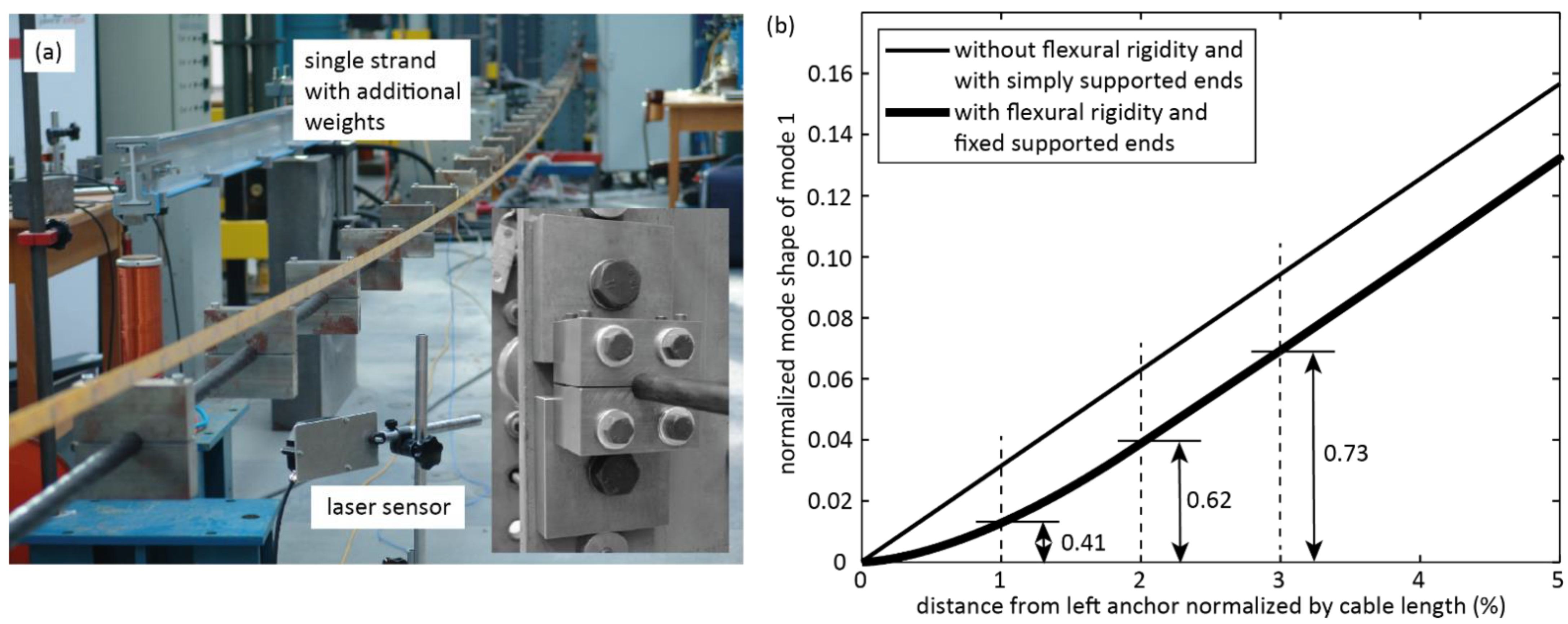
2.2. Cable with Flexural Rigidity and Fixed Supported Ends

Modeshape measurements on a single steel strand with seven wires and fixed support ends were performed using a laser-based displacement sensor (Figure 2a). The length of the steel wire strand was approximately 15.5 m and the mass per unit length including the additional masses was approximately 1.17 kg/m and the pre-stressing force was approximately 33 kN. The measured modeshape, which can be described by sinus-hyperbolics and cosine-hyperbolics functions, clearly deviates from the sinusoidal modeshape function being valid for a taut string with simply supported ends and without flexural rigidity (Figure 2b). The measurements show that the transverse cable motion especially deviates from the sinusoidal modeshape between the anchor and approximately 5% of the cable length which is the range where transverse dampers are commonly positioned. If the cable model includes the fixed end conditions and the flexural rigidity, the cable can be modelled by the beam modelling approach

$$E I \frac{{\partial }^{4}v\left(x,t\right)}{\partial x^4}+T \frac{{\partial }^{2}v\left(x,t\right)}{\partial x^2}-m \frac{{\partial }^{2}v\left(x,t\right)}{\partial t^2}=f \delta \left(x-a\right)$$

(4)

where E is the elastic modulus of the cable and I is the second moment of area. The boundary conditions for the case of the fixed supported ends are as follows:

$$v\left(x=0,t\right)=0, \frac{\partial v\left(x=0,t\right)}{\partial x}=0, v\left(x=L,t\right)=0,\frac{\partial v\left(x=L,t\right)}{\partial x}=0$$

(5)

These boundary conditions mean that the bending moments at both cable ends are not zero which leads to modeshape functions based on a linear combination of sine-hyperbolic, cosine-hyperbolic, sine and cosine functions

$$V_n\left(x\right)=-\frac{{\alpha }_n}{{\beta }_n} sinh\left({\beta }_n x\right)-\frac{1}{{\theta }_n} cosh\left({\beta }_n x\right)+sin\left({\beta }_n x\right)+\frac{1}{{\theta }_n} cos\left({\beta }_n x\right)$$

(6)

$${\theta }_n=\frac{{\beta }_n sinh\left({\beta }_n L\right)+{\alpha }_n sin\left({\alpha }_n L\right)}{-{\alpha }_n cosh\left({\beta }_n L\right)+{\alpha }_n cos\left({\alpha }_n L\right)}$$

(7)

where ${\alpha }_{1}L=$3.181 and ${\beta }_{1}L=$1.624 etc., see [23]. This cable model is validated by adjusting $E I$ to obtain the measured modeshape.

2.3. Cable Model for Simulation

For the simulation of the cable model with transverse damper, the partial differential Equations (1) and (3) are discretized, adopting a finite truss element modelling approach with the spatial sampling interval $\mathsf{\Delta }x\ll L$ that is selected small enough to ensure precise approximation of the partial differential Equations (1) and (3) [24,34,35,45]

$$\mathrm{M} \ddot{\mathrm{v}}+\mathrm{C} \mathrm{v} \dot{}+\mathrm{K} \mathrm{v}=\mathsf{\phi } f\left(t\right)+{\mathrm{F}}_{\mathrm{ex}}$$

(8)

where M, C and K denote the mass, damping and stiffness matrices, v is the vector of the transverse displacements, $\mathsf{\phi }$ is the connectivity vector of the transverse damper force and the excitation force vector F_ex is introduced to excite the cable model harmonically at the eigenfrequencies of the considered modes. The inherent cable damping ratio ${\xi }_{cable}$ is assumed to be 0.4% which is a typical value of the first few modes of stay cables [2,29,30].

2.4. Optimum Viscous Damper for One Targeted Mode and Taut String Behaviour

The force of the passive transverse damper is assumed to produce linear viscous damping

$$f\left(t\right)=-c \frac{\partial v\left(a,t\right)}{\partial t}$$

(9)

where c denotes the viscous damper coefficient in (Ns/m). According to the literature [14,15,16], the optimum value of c for maximum damping in mode n and assuming that the cable dynamics can be described by the taut string model is given as follows

$$c=c_n^{opt}=\frac{T}{a {\omega }_n}$$

(10)

where ${\omega }_n$ denotes the eigenfrequency in rad/s of mode n. The resulting damping ratio in mode n is given by the simple approximation

$${\zeta }_n\approx \frac{1}{2}\frac{a}{L}$$

(11)

The expressions (10) and (11) are only valid for a taut string, i.e., a cable with simply supported ends and without flexural rigidity, and a transverse damper being optimized to one targeted mode and not to several modes as commonly specified for real stay cables.

2.5. Optimum Viscous Damper for Several Targeted Modes and Taut String Behaviour

Cable dampers are always specified to provide at least the required damping ratio in several targeted modes, e.g., the first four modes. Then, the solution (10), which maximizes the damping in one targeted mode, does not yield the optimum tuning of the transverse damper. As shown in [19], the optimum tuning of c targeting several modes is obtained by equating the damping ratios in the lowest (mode number i) and highest (mode number j) targeted modes and setting these damping ratios equal to the required damping ratio ${\zeta }_{req}$. Then, the optimum of the viscous damper coefficient for maximum damping of modes i to j becomes

$$c={\left(c_{i-j}^{opt}\right)}_{\min \left(a\right)}=\frac{T}{{\zeta }_{req}L {\omega }_1\left(i+j\right)}$$

(12)

The according damper position is automatically minimized because the damping ratios of the lowest and highest targeted modes just meet ${\zeta }_{req}$, that is

$${\left(\frac{a_{min}}{L}\right)}_{i-j}=\frac{{\zeta }_{req }\left(i+j\right)}{\sqrt{i j }}$$

(13)

The resulting damping ratio in mode n then becomes

$${\left({\zeta }_{i-j}^{\min \left(a\right)}\right)}_n=\frac{{\zeta }_{req }n \left(i+j\right)}{n^2+i j}$$

(14)

3. Semi-Active Cable Damper

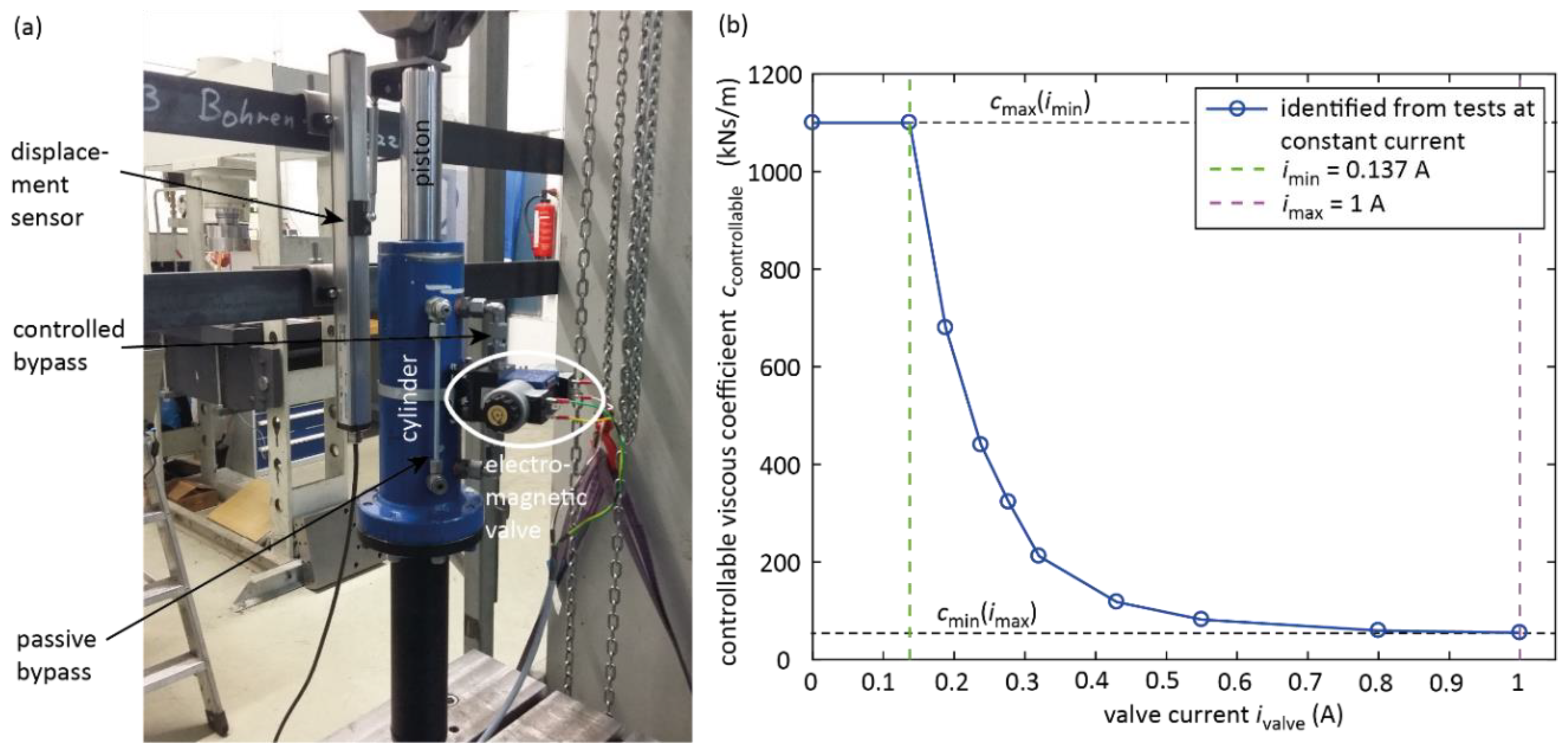
3.1. System Description

The semi-active damper is realized using a conventional passive oil damper which is enriched by a controlled bypass with electromagnetic valve (Figure 3a). To limit the maximum viscous force at fully closed bypass valve, a small passive bypass is added. The oil volume stream of this passive bypass valve and therefore the maximum oil damper force is tuned by a passive throttle within the passive bypass. The controlled bypass valve in combination with the passive bypass generate quadratic viscous damping because both bypasses act as throttles. The controllable viscous coefficient as function of the applied electromagnetic valve current defines the control force range between the minimum and the maximum viscous coefficients; the according look-up table data is depicted in Figure 3b. The control law of clipped viscous damping with negative stiffness is computed based on the collocated relative damper motion, which is measured by the displacement sensor measuring the relative motion between damper cylinder and damper piston and which is equal to the transverse cable motion at damper position.

3.2. Control Law

The control law is semi-active linear viscous damping with negative stiffness (clipped VDNS), which can be realized by collocated control and is proven to be a very efficient damping algorithm (Figure 1b and Figure 4, [24,38,39]). The high damping efficiency of clipped VDNS is explained by the fact that VDNS combines energy dissipation by the viscous force while the negative stiffness force increases the relative motion of the damper which leads to increased cycle energy within the damper. In addition, the control force characteristics of VDNS are similar to those resulting from optimal control as shown in [24]. For these two reasons, i.e., enlarged damper relative motion due to the negative stiffness force and optimal control similarity, VDNS is a very effective damping strategy. Further benefits are that VDNS does not require a state observer as optimal control does and that it works for any type of excitation, i.e., for single harmonic, narrow and broad band excitations because the desired semi-active control force can be computed in real time based on the measured actual damper motion only. In the following, the most relevant steps of the control law computation are explained. The viscous damping coefficient $c_{frequency}^{opt}$ is adjusted in real time to the actual frequency of vibration in order to generate optimum modal damping (15). The negative stiffness coefficient $k$ is formulated based on the known parameters T and a [46]. The two tuning parameters $g_1$ and $g_2$ are needed to compensate for the damping increase and stiffness loss due to the clipping of the active desired control force; more information on undesired damping increase and stiffness loss due to clipping can be found in [47]. Reasonable values for $g_1$ and $g_2$ are 0.80 and 1.20 [46]. The main modules of the control algorithm are shortly described here (Figure 4):

• Bandpass filtering of damper relative motion (displacement sensor signal, Figure 3a) to remove offset and noise in the displacement signal.
• Derivation of damper relative velocity by numeric differentiation with subsequent low pass filtering to attenuate noise due to the numeric differentiation.
• Frequency detection from the peaks of the displacement signal resulting in a maximum time delay of half a period. This time delay is more than acceptable considering that resonant vibrations are long standing vibrations, see cable vibration measurements presented in [30].
• Computing the desired active control force $f_{des}^{active}$ (17) and the desired semi-active control force $f_{des}^{semi\text{-}active}$ (18).
• The control force tracking task is solved in two steps. First, the desired viscous coefficient c_des(t) of the controllable damper is computed based on the desired semi-active control force (19) and the actual damper relative velocity, then the desired current of the electromagnetic valve is computed based on the steady state relation between valve current and viscous damper coefficient (Figure 3a, (20)). Equation (19) shows that the controllable damper exerts quadratic viscous damping at constant bypass valve position, i.e., at constant valve current, because both the controlled bypass valve and the passive bypass act as throttles resulting in quadratic viscous damping.
• The PID-based current controller including an anti-reset windup (ARW) due to the current limitations ensures that the actual valve current precisely tracks the desired current $i_{des}$.
• The state variables, which are given as function of time t in (15)–(20), are computed in real time at the controller frequency of 1000 Hz.
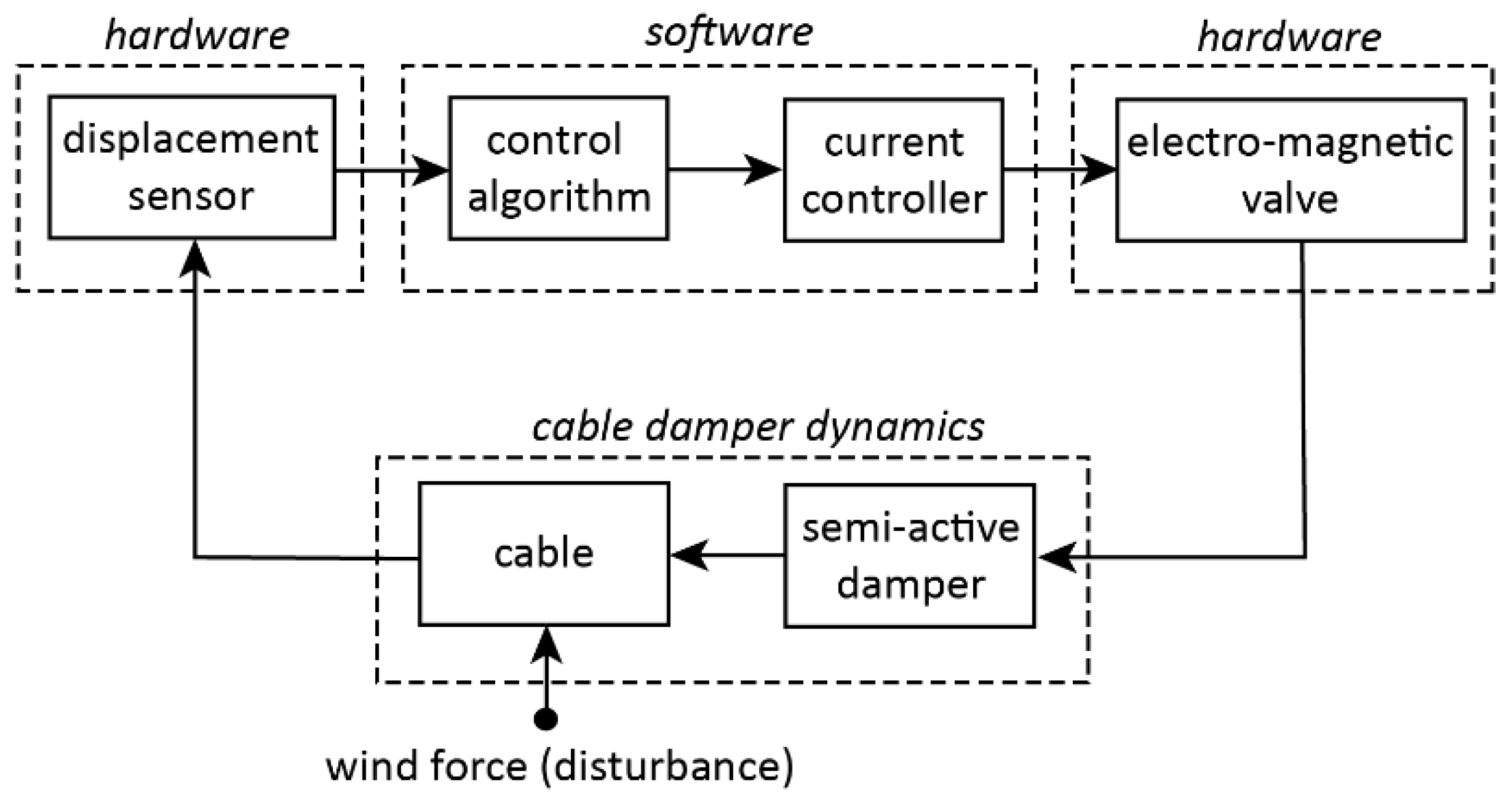
• The closed-loop structure consisting of hardware components, software components and cable damper dynamics is depicted in Figure 5.

$$c_{frequency}^{opt}\left(t\right)=g_1\frac{T}{ a \left(2 \pi frequency\left(t\right)\right)}$$

(15)

$$k=g_2 \frac{T}{a}$$

(16)

$$f_{des}^{active}\left(t\right)=-\left\{c_{frequency}^{opt}\left(t\right) \frac{dv\left(a,t\right)}{dt}-k v\left(a,t\right)\right\}$$

(17)

$$f_{des}^{semi\text{-}active}\left(t\right)=\{\begin{array}{cc}{f}_{des}^{active}\left(t\right)& : f_{des}^{active}\left(t\right) \frac{dv\left(a,t\right)}{dt}\le 0\\ 0& : f_{des}^{active}\left(t\right) \frac{dv\left(a,t\right)}{dt}>0\end{array}$$

(18)

$$c_{des}\left(t\right)=\frac{\left| f_{des}^{semi\text{-}active}\left(t\right)\right|}{{\left(\frac{dv\left(a,t\right)}{dt}\right)}^2}$$

(19)

$$i_{des}\left(t\right)=function\left(c_{des}\left(t\right), c_{min},c_{max}\right)$$

(20)

3.3. Experimental Validation

The control algorithm described in 3.2 is experimentally validated with an active hydraulic damper imposing a displacement with defined frequency and amplitude into the semi-active damper, see Figure 3a. The goal of this experiment is to determine the real-time force tracking accuracy without using a force sensor (no force feedback in the algorithm) in order to save the costs of a load cell for each semi-active cable damper. The test results at the amplitude of 20 mm and the frequency of 0.27 Hz are depicted by the force displacement and force velocity curves of the desired semi-active control force and the actual force of the semi-active damper in Figure 6. The experimental results demonstrate that the force tracking error between the desired semi-active control force and the actual semi-active force are predominantly caused by the minimum and maximum viscous coefficients resulting from the fully open and fully closed electromagnetic valve. These force tracking errors cannot be avoided even with force feedback because the minimum and maximum viscous coefficients determine the force limitations of the controllable damper.

3.4. Modell of Semi-Active Damper Force including Force Limitations

For the simulations of the cable model with semi-active damper, the actual force of the semi-active damper is modelled by the actual semi-active control force that is equal to the desired semi-active control force, including the force limitations due to the minimum and maximum viscous coefficients at fully open and fully closed bypass valve, i.e., at maximum and minimum valve currents, see Figure 3b (21).

$$\begin{array}{l}{f}_{actual}^{semi\text{-}active}(t)\\ =\{\begin{array}{l}sign\left(\frac{dv(a,t)}{dt}\right)c_{min}{\left(\frac{dv(a,t)}{dt}\right)}^2\hspace{1em}\hspace{1em}\hspace{1em}:|f_{des}^{semi\text{-}active}(t)|<c_{min}{\left(\frac{dv(a,t)}{dt}\right)}^2\\ \hspace{1em}\hspace{1em}\hspace{1em}{f}_{des}^{semi\text{-}active}(t)\hspace{1em}\hspace{1em}\hspace{1em}:c_{min}{\left(\frac{dv(a,t)}{dt}\right)}^2\le |f_{des}^{semi\text{-}active}(t)|\le c_{max}{\left(\frac{dv(a,t)}{dt}\right)}^2\\ sign\left(\frac{dv(a,t)}{dt}\right)c_{max}{\left(\frac{dv(a,t)}{dt}\right)}^2\hspace{1em}\hspace{1em}\hspace{1em}:|f_{des}^{semi\text{-}active}(t)|>c_{max}{\left(\frac{dv(a,t)}{dt}\right)}^2\end{array}\end{array}$$

(21)

4. Simulation results

4.1. Assumptions, Cable Properties

The simulations with transverse damper are performed for the following damper types, assumptions, vibration modes, cable properties and damper positions:

• Damper types:

  -

  Passive linear viscous damper being optimized to one targeted mode, i.e., the excited mode, which represents a theoretical benchmark as passive dampers always need to mitigate several targeted modes.

  -

  Passive linear viscous damper being optimized to the targeted modes 1 to 4 describing the realistic benchmark.

  -

  Semi-active damper controlled by clipped VDNS including the control force constraints due to the minimum and maximum controllable viscous coefficients.

• The vibration mitigation of the considered transverse dampers are computed for the first four cable modes.
• Single mode vibrations are considered as resonant vibrations result in greatest cable displacement amplitudes.
• The excitation force due to vortex-shedding is modelled as harmonic excitation.
• The simulations are performed assuming typical cable properties and typical damper positions:

  -

  Cable length L = 300 m.

  -

  Cable tension force T = 6700 kN.

  -

  Mass per unit length m = 100 kg/m.

  -

  First eigenfrequency f₁ = 0.431 Hz (determined by L, T, m).

  -

  Inherent cable damping ratio ζ_cable= 0.4%.

  -

  Relative damper positions a/L = 1%, 1.67%, 2%, 2.5% and 3%.

4.2. Excitation Force Amplitude

The excitation force amplitude is selected to obtain L/1700 anti-node displacement amplitude V_n during steady state conditions to ensure that the semi-active damper including control force constraints is operated in the typical range of damper relative velocities with associated typical semi-active damper forces. After reaching steady state vibrations, the excitation force is turned off to simulate the free decay response (Figure 7).

4.3. Damper Performance Assessment from Free Decay Response

The efficiencies of the passive damper and of the semi-active damper with control force constraints are assessed from simulated free decay responses adopting the logarithmic decrement method

$${\delta }_i=ln\left(\frac{V_i}{V_{i+1}}\right)$$

(22)

where V_i denotes the anti-node cable displacement amplitude of period i during the free decay response and V_i+1 is the anti-node amplitude of the subsequent period. This yields the damping ratio as follows

$${\zeta }_i=\frac{{\delta }_i}{\sqrt{4 {\pi }^2+{\delta }^2}}-{\zeta }_{cable}$$

(23)

where the cable inherent damping ratio is subtracted from the damping ratio obtained from the free decay response.

The damping assessment from the free decay response is selected because the cable damping due to the semi-active damper cannot be determined in a different way due to the nonlinearities of clipping and control force constraints. Because of these nonlinearities the peak-to-peak damping ratio is not fully constant as for linear transverse cable dampers. Therefore, the damping of the free decay response is assessed from the exponential fit of the free decay response between decay start and 10% of the steady state amplitude [29,30,34]. Figure 7 depicts examples of the exponential fits for a passive damper being optimized to the excited mode (10), a passive damper being optimized to the first four targeted modes (12) and for the semi-active damper with the consideration of the control force constraints. Figure 7c shows that the local peaks during the free decay response match well the exponential fit. Hence, the nonlinearities due to clipping and control force limitations of the semi-active damper are minor and therefore do not falsify the damping determination by the exponential fit method.

4.4. Damper Efficiency

The efficiency $\eta$ of the transverse dampers is determined by comparing the damping ratio obtained from the exponential fit of the free decay response with the theoretical damping ratio due to linear viscous damping being optimized to one target mode

$$\eta =\frac{\left({\zeta }_{fit}-{\zeta }_{cable}\right)-{\zeta }_{num}}{\raisebox{1ex}{$1$}\!\left/ \!\raisebox{-1ex}{$2$}\right. \frac{a}{L}}$$

(24)

The numerical damping ${\zeta }_{num}$, which is subtracted from $({\zeta }_{fit}-{\zeta }_{cable})$, is determined for the simulation case of optimum modal linear viscous damping for which the resulting damping ratio is known by the analytical expression $L/\left(2 a\right)$ where L denotes the half wavelength [14,15,16]. Note that the numerical damping of significantly less than 0.1% results from any integration algorithm and therefore cannot be avoided.

4.5. Results

The damping ratio due to the damper (including the numerical damping) and the according damper efficiency (24, without numerical damping) are given in

Table 1. Results for mode 1 excited.

Damper Type	Cable Model	a/L (%)	${\mathit{\zeta }}_{\mathit{f}\mathit{i}\mathit{t}}-{\mathit{\zeta }}_{\mathit{c}\mathit{a}\mathit{b}\mathit{l}\mathit{e}} (\%)$	${\mathit{\zeta }}_{\mathit{n}\mathit{u}\mathit{m}} (\%)$	½ a/L	η (%)
passive, tuned to mode 1	taut string	1%	0.505%	0.005% (*)	0.5%	100% (*)
	FR & FSC		0.354%			69.8%
passive, tuned to modes 1–4	taut string		0.403%			79.6%
	FR & FSC		0.198%			38.6%
semi-active	taut string		1.036%			206.2%
	FR & FSC		0.571%			113.2%
passive, tuned to mode 1	taut string	1.67%	0.848%	0.013% (*)	0.84%	100% (*)
	FR & FSC		0.716%			84.2%
passive, tuned to modes 1–4	taut string		0.675%			79.3%
	FR & FSC		0.431%			50.1%
semi-active	taut string		1.723%			204.8%
	FR & FSC		1.310%			155.3%
passive, tuned to mode 1	taut string	2%	1.021%	0.021% (*)	1%	100% (*)
	FR & FSC		0.912%			89.1%
passive, tuned to modes 1–4	taut string		0.811%			79.0%
	FR & FSC		0.570%			54.9%
semi-active	taut string		2.058%			203.7%
	FR & FSC		1.790%			176.9%
passive, tuned to mode 1	taut string	2.5%	1.284%	0.034% (*)	1.25%	100% (*)
	FR & FSC		1.194%			92.8%
passive, tuned to modes 1–4	taut string		1.017%			78.6%
	FR & FSC		0.775%			59.3%
semi-active	taut string		2.636%			208.2%
	FR & FSC		2.395%			188.9%
passive, tuned to mode 1	taut string	3%	1.549%	0.049% (*)	1.5%	100% (*)
	FR & FSC		1.471%			94.8%
passive, tuned to modes 1–4	taut string		1.224%			78.3%
	FR & FSC		0.978%			61.9%
semi-active	taut string		3.169%			208.0%
	FR & FSC		3.014%			197.7%

(*) numerical damping determined from ${\zeta }_{fit}$ due to passive viscous damping optimized to excited mode to obtain η = 100%.

,

Table 2. Results for mode 2 excited.

Damper Type	Cable Model	a/L (%)	${\mathit{\zeta }}_{\mathit{f}\mathit{i}\mathit{t}}-{\mathit{\zeta }}_{\mathit{c}\mathit{a}\mathit{b}\mathit{l}\mathit{e}} (\%)$	${\mathit{\zeta }}_{\mathit{n}\mathit{u}\mathit{m}} (\%)$	½ a/L	η (%)
passive, tuned to mode 2	taut string	1%	0.506%	0.006% (*)	0.5%	100% (*)
	FR & FSC		0.354%			69.6%
passive, tuned to modes 1–4	taut string		0.506%			100.0%
	FR & FSC		0.354%			69.6%
semi-active	taut string		1.025%			203.8%
	FR & FSC		0.571%			113.0%
passive, tuned to mode 2	taut string	1.67%	0.849%	0.014% (*)	0.84%	100% (*)
	FR & FSC		0.716%			84.1%
passive, tuned to modes 1–4	taut string		0.849%			100.0%
	FR & FSC		0.716%			84.1%
semi-active	taut string		1.732%			205.7%
	FR & FSC		1.342%			159.0%
passive, tuned to mode 2	taut string	2%	1.023%	0.023% (*)	1%	100% (*)
	FR & FSC		0.913%			89.0%
passive, tuned to modes 1–4	taut string		1.023%			100.0%
	FR & FSC		0.913%			89.0%
semi-active	taut string		2.083%			206.0%
	FR & FSC		1.807%			178.4%
passive, tuned to mode 2	taut string	2.5%	1.288%	0.038% (*)	1.25%	100% (*)
	FR & FSC		1.196%			92.6%
passive, tuned to modes 1–4	taut string		1.288%			100.0%
	FR & FSC		1.196%			92.6%
semi-active	taut string		2.574%			202.9%
	FR & FSC		2.461%			193.8%
passive, tuned to mode 2	taut string	3%	1.557%	0.057% (*)	1.5%	100% (*)
	FR & FSC		1.474%			94.5%
passive, tuned to modes 1–4	taut string		1.557%			100.0%
	FR & FSC		1.474%			94.5%
semi-active	taut string		3.083%			201.7%
	FR & FSC		3.081%			201.6%

(*) numerical damping determined from ${\zeta }_{fit}$ due to passive viscous damping optimized to excited mode to obtain η = 100%.

,

Table 3. Results for mode 3 excited.

Damper Type	Cable Model	a/L (%)	${\mathit{\zeta }}_{\mathit{f}\mathit{i}\mathit{t}}-{\mathit{\zeta }}_{\mathit{c}\mathit{a}\mathit{b}\mathit{l}\mathit{e}} (\%)$	${\mathit{\zeta }}_{\mathit{n}\mathit{u}\mathit{m}} (\%)$	½ a/L	η (%)
passive, tuned to mode 3	taut string	1%	0.506%	0.006% (*)	0.5%	100% (*)
	FR & FSC		0.354%			69.6%
passive, tuned to modes 1–4	taut string		0.465%			91.8%
	FR & FSC		0.452%			89.2%
semi-active	taut string		0.975%			193.8%
	FR & FSC		0.567%			112.2%
passive, tuned to mode 3	taut string	1.67%	0.851%	0.016% (*)	0.84%	100% (*)
	FR & FSC		0.716%			83.8%
passive, tuned to modes 1–4	taut string		0.782%			91.7%
	FR & FSC		0.836%			98.2%
semi-active	taut string		1.655%			196.3%
	FR & FSC		1.318%			155.9%
passive, tuned to mode 3	taut string	2%	1.028%	0.028% (*)	1%	100% (*)
	FR & FSC		0.913%			88.5%
passive, tuned to modes 1–4	taut string		0.944%			91.6%
	FR & FSC		1.025%			99.7%
semi-active	taut string		1.980%			195.2%
	FR & FSC		1.761%			173.3%
passive, tuned to mode 3	taut string	2.5%	1.296%	0.046% (*)	1.25%	100% (*)
	FR & FSC		1.199%			92.2%
passive, tuned to modes 1–4	taut string		1.190%			91.5%
	FR & FSC		1.295%			99.9%
semi-active	taut string		2.403%			188.6%
	FR & FSC		2.319%			181.8%
passive, tuned to mode 3	taut string	3%	1.569%	0.069% (*)	1.5%	100% (*)
	FR & FSC		1.481%			94.1%
passive, tuned to modes 1–4	taut string		1.442%			91.5%
	FR & FSC		1.563%			99.6%
semi-active	taut string		2.833%			184.3%
	FR & FSC		2.924%			190.3%

(*) numerical damping determined from ${\zeta }_{fit}$ due to passive viscous damping optimized to excited mode to obtain η = 100%.

and

Table 4. Results for mode 4 excited.

Damper Type	Cable Model	a/L (%)	${\mathit{\zeta }}_{\mathit{f}\mathit{i}\mathit{t}}-{\mathit{\zeta }}_{\mathit{c}\mathit{a}\mathit{b}\mathit{l}\mathit{e}} (\%)$	${\mathit{\zeta }}_{\mathit{n}\mathit{u}\mathit{m}} (\%)$	½ a/L	η (%)
passive, tuned to mode 4	taut string	1%	0.507%	0.007% (*)	0.5%	100% (*)
	FR & FSC		0.354%			69.4%
passive, tuned to modes 1–4	taut string		0.402%			79.0%
	FR & FSC		0.497%			98.0%
semi-active	taut string		0.949%			188.4%
	FR & FSC		0.557%			110.0%
passive, tuned to mode 4	taut string	1.67%	0.855%	0.020% (*)	0.84%	100% (*)
	FR & FSC		0.715%			83.2%
passive, tuned to modes 1–4	taut string		0.675%			78.4%
	FR & FSC		0.850%			99.4%
semi-active	taut string		1.647%			194.9%
	FR & FSC		1.290%			152.1%
passive, tuned to mode 4	taut string	2%	1.033%	0.033% (*)	1%	100% (*)
	FR & FSC		0.914%			88.1%
passive, tuned to modes 1–4	taut string		0.814%			78.1%
	FR & FSC		1.009%			97.6%
semi-active	taut string		1.954%			192.1%
	FR & FSC		1.761%			172.8%
passive, tuned to mode 4	taut string	2.5%	1.308%	0.058% (*)	1.25%	100% (*)
	FR & FSC		1.204%			91.7%
passive, tuned to modes 1–4	taut string		1.029%			77.7%
	FR & FSC		1.242%			94.7%
semi-active	taut string		2.419%			188.9%
	FR & FSC		2.346%			183.0%
passive, tuned to mode 4	taut string	3%	1.590%	0.090% (*)	1.5%	100% (*)
	FR & FSC		1.488%			93.2%
passive, tuned to modes 1–4	taut string		1.245%			77.0%
	FR & FSC		1.475%			92.3%
semi-active	taut string		2.842%			183.5%
	FR & FSC		2.954%			190.9%

(*) numerical damping determined from ${\zeta }_{fit}$ due to passive viscous damping optimized to excited mode to obtain η = 100%.

for modes 1 to 4 as function of:

• Damper types:

  -

  Passive, tuned to mode X (1, 2, 3, 4): linear viscous damper being optimized to the excited mode (19); this is a theoretical benchmark because transverse cable dampers always need to provide the specified damping in several targeted modes; this computation is required to determine the numerical damping.

  -

  Passive, m1-m4: linear viscous damper being optimized to the targeted modes 1–4 (12).

  -

  Semi-active: clipped VDNS including control force constraints due to c_min and c_max (21).

• Cable model:

  -

  Taut string: cable without flexural rigidity and simply supported ends.

  -

  FR and FSC: cable with flexural rigidity and fixed support end conditions.

• Relative damper positions a/L = 1%, 1.67%, 2%, 2.5% and 3%.

The observation of Table 1, Table 2, Table 3 and Table 4 reveals the following main findings:

• The reduced cable motion at damper position due to cable flexural rigidity and fixed supported ends has strong impact on the cable damping ratio due to passive dampers located at a/L ≤ 2%. This fact is explained by the associated reduced transverse damper motion, see Figure 2b, whereby less energy per cycle can be dissipated.
• The damper efficiencies obtained from the simulation case of a cable with flexural rigidity and fixed supported ends, mode 1 excited, typical damper positions around 2% to 2.5% and passive damper being optimized to modes 1–4 match well with the reported damper efficiencies [23,24,25,26,27,28,29,30,31]. The according results for mode 2 are greater because a damper being optimized to modes 1–4 generates optimum damping in mode 2 (14), see [19]. In this perspective the according simulation results for modes 3 and 4 of the cable model with bending stiffness and fixed support conditions (FR and FSC) seem to be unrealistically high. This irrational result is interpreted by the fact that the cable model FR and FSC is validated for the modeshape of mode 1 of the test steel wire strand depicted in Figure 2 but not for higher modes.
• For some simulation cases, the damping of the cable model with flexural rigidity and fixed supported ends is greater than for the taut string model. This unexpected result is observed for some simulations of modes 3 and 4 and mainly for the passive damper being optimized to modes 1 to 4. An explanation can be that the reduced cable motion at damper position reduces the damper velocity as well whereby the viscous coefficient being optimized for modes 1 to 4 (12) almost generates the optimum viscous force for modes 3 and 4.
• The damping results due to the semi-active damper with the consideration of the minimum and maximum force limitations due to fully open and fully closed bypass valve show the following picture:

  -

  Mode 1: The damping is approximately 2.5…2.6 (taut string) and approximately 2.8…3.2 (FR and FSC) times greater than the damping due to the passive damper being optimized to modes 1 to 4.

  -

  Mode 2: The damping is approximately 2.0…2.6 (taut string) and approximately 1.6…2.1 (FR and FSC) times greater than the damping due to the passive damper being optimized to modes 1 to 4.

  -

  Mode 3: The damping is approximately 2.0…2.1 (taut string) and approximately 1.3…1.9 (FR and FSC) times greater than the damping due to the passive damper being optimized to modes 1 to 4.

  -

  Mode 4: The damping is approximately 2.3…2.5 (taut string) and approximately 1.2…2.1 (FR and FSC) times greater than the damping due to the passive damper being optimized to modes 1 to 4.

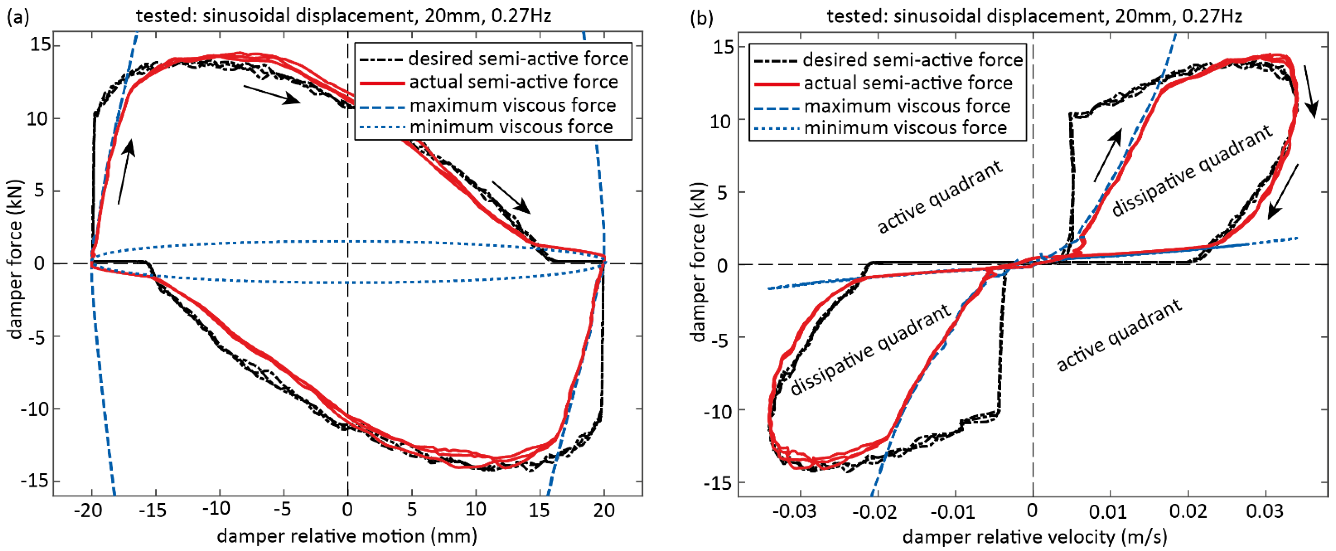
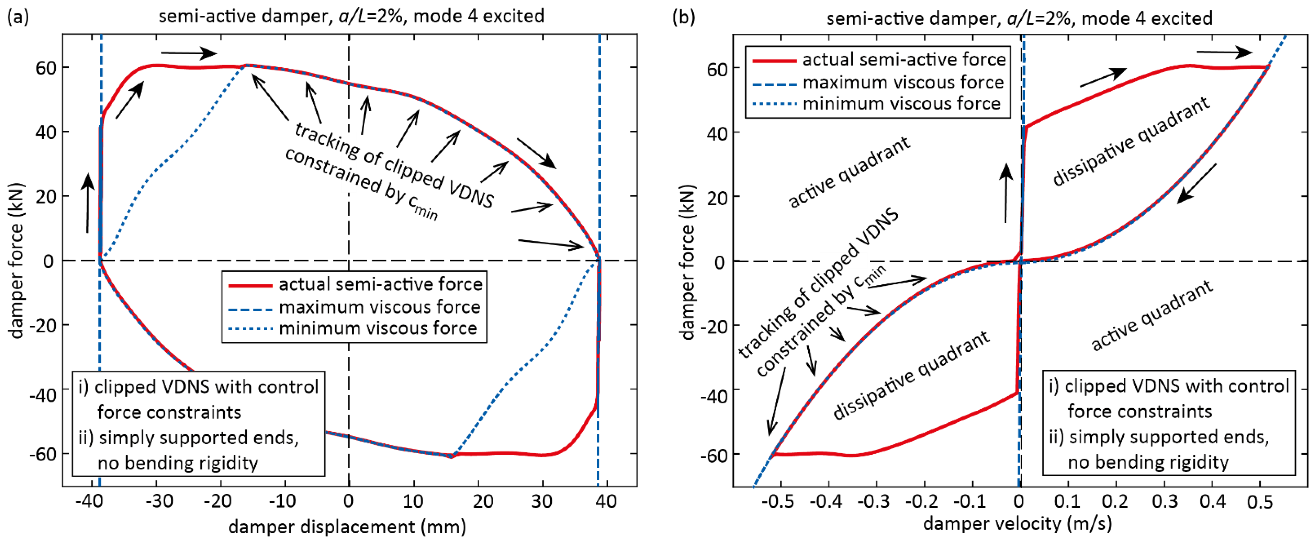
• The tracking of the desired semi-active force is limited by the minimum and maximum viscous coefficients of the controllable damper. The according force displacement curves due to the minimum and maximum quadratic viscous forces are depicted in Figure 8 and Figure 9 for the simulations of mode 1 and 4. It is observed that c_max mainly constrains the force tracking accuracy for lower frequency modes while c_min mainly limits the force tracking accuracy for higher frequency modes. This is explained by the fact that the according limiting control forces are in proportion to the square of the damper relative velocity, see (21). Hence, how precisely the desired semi-active force can be tracked by the semi-active damper with control force limitations due to c_min and c_max depends on mode number, which makes the interpretation of the obtained cable damping results for modes 3 and 4 difficult.

5. Conclusions

This study investigates the potential to use semi-active cable dampers controlled by clipped viscous damping with negative stiffness to compensate for the reduced cable motion at damper position due to cable flexural rigidity and fixed supported ends. For this a prototype hydraulic damper with real-time controlled bypass valve has been developed and experimentally tested. Based on the test results a model of the semi-active hydraulic damper is derived that includes the control force constraints resulting from the minimum and maximum viscous coefficients at fully open and fully closed bypass valve. This model is used to compute the cable damping ratios of the first four cable modes, typical damper positions and cable models without and with flexural rigidity and fixed supported ends. As benchmark, the passive damper being optimized to the first four cable modes is computed. The comparative study demonstrates that the presented semi-active cable damper leads to far greater cable damping ratios than the passive damper. This is explained by the facts that the viscous force is optimized in real time to the actual frequency of motion and the negative stiffness force increases the damper relative motion whereby the viscous force can dissipate more energy per cycle. Because of the dissipative nature of the semi-active damper force, stability issues as for active systems do not exist. In addition, power consumption is not critical because power is only needed to control the oil volume stream through the bypass valve but not to produce active forces. Therefore, the presented semi-active hydraulic damper represents an efficient, cost-effective and robust damping tool for stay cable damping.

References

1. Fib Bulletin 30. Acceptance of stay cable systems using prestressing steels. In Bulletin 30; International Federation for Structural Concrete Fib: Lausanne, Switzerland, 2005; ISBN 2-88394-070-3. [Google Scholar]
2. Jain, A.; Simsir, C.; Sarkar, P.P. Analysis, Measurement, and Mitigation of Stay Cable Vibrations. Eighth Congr. Forensic Eng. 2018, 791–799. [Google Scholar] [CrossRef]
3. Matsumoto, M.; Saitoh, T.; Kitazawa, M.; Shirato, H.; Nishizaki, T. Response characteristics of rain-wind induced vibration of stay-cables of cable-stayed bridges. J. Wind Eng. Ind. Aerodyn. 1995, 57, 323–333. [Google Scholar] [CrossRef]
4. Zuo, D.; Jones, N.P. Interpretation of field observations of wind- and rain-wind-induced stay cable vibrations. J. Wind Eng. Ind. Aerodyn. 2010, 98, 73–87. [Google Scholar] [CrossRef]
5. Li, S.; Chen, Z.; Wu, T.; Kareem, A. Rain-wind-induced in-plane and out-of-plane vibrations of stay cables. J. Eng. Mech. 2013, 139, 1688–1698. [Google Scholar] [CrossRef]
6. Wang, H.; Li, A.; Niu, J.; Zong, Z.; Li, J. Long-term monitoring of wind characteristics at Sutong Bridge site. J. Wind Eng. Ind. Aerodyn. 2013, 115, 39–47. [Google Scholar] [CrossRef]
7. Guo, J.; Zhu, X. Field Monitoring and Analysis of the Vibration of Stay Cables under Typhoon Conditions. Sensors 2020, 20, 4520. [Google Scholar] [CrossRef] [PubMed]
8. Vo-Duy, H.; Nguyen, C.H. Vibration Control Techniques for Dynamic Response Mitigation of Civil Structures under Multiple Hazards. Shock Vib. 2020, 2020, 5845712. [Google Scholar] [CrossRef]
9. Daniottia, N.; Jakobsen, J.B.; Snæbjörnsson, J.; Cheynet, E.; Wang, J. Observations of bridge stay cable vibrations in dry and wet conditions: A case study. J. Sound Vib. 2021, 503, 116106. [Google Scholar] [CrossRef]
10. An, M.; Li, S.; Liu, Z.; Yan, B.; Li, L.; Chen, Z. Galloping vibration of stay cable installed with a rectangular lamp: Field observations and wind tunnel tests. J. Wind Eng. Ind. Aerodyn. 2021, 215, 104685. [Google Scholar]
11. Ni, Y.Q.; Wang, X.Y.; Chen, Z.Q.; Ko, J.M. Field observations of rain-wind-induced cable vibration in cable-stayed Dongting Lake Bridge. J. Wind Eng. Ind. Aerodyn. 2007, 95, 303–328. [Google Scholar] [CrossRef]
12. Savor, Z.; Radic, J.; Hrelja, G. Cable vibrations at Dubrovnik bridge. Bridge Struct. 2006, 2, 97–106. [Google Scholar] [CrossRef]
13. Casas, J.R.; Aparicio, A.C. Rain-wind-induced cable vibrations in the Alamillo cable-stayed bridge (Sevilla, Spain). Assessment and remedial action. Struct. Infrastruct. Eng. 2010, 6, 549–556. [Google Scholar] [CrossRef] [Green Version]
14. Pacheco, B.M.; Fujino, Y.; Sulekh, A. Estimation curve for modal damping in stay cables with viscous damper. J. Struct. Eng. 1993, 119, 1961–1979. [Google Scholar] [CrossRef]
15. Krenk, S. Vibrations of a taut cable with an external damper. J. Appl. Mech. 2000, 67, 772–776. [Google Scholar] [CrossRef]
16. Main, J.A.; Jones, N.P. Free vibrations of taut cable with attached damper. I: Linear viscous damper. J. Eng. Mech. 2002, 128, 1062–1071. [Google Scholar] [CrossRef] [Green Version]
17. Krenk, S.; Høgsberg, J.R. Damping of cables by a transverse force. J. Eng. Mech. 2005, 131, 340–348. [Google Scholar] [CrossRef]
18. Fujino, Y.; Siringoringo, D. Vibration Mechanisms and Controls of Long-Span Bridges: A Review. Struct. Eng. Int. 2013, 23, 248–268. [Google Scholar] [CrossRef]
19. Weber, F.; Feltrin, G.; Maślanka, M.; Fobo, W.; Distl, H. Design of viscous dampers targeting multiple cable modes. Eng. Struct. 2009, 31, 2797–2800. [Google Scholar] [CrossRef]
20. Hoang, N.; Fujino, Y. Analytical study on bending effects in a stay cable with a damper. J. Eng. Mech. 2007, 133, 1241–1246. [Google Scholar] [CrossRef]
21. Hammoudi, Z.S.; Abbas, A.L.; Mahmood, H.A. Free Vibration Analysis of Cable Stayed-Bridge by Finite Element Method. Diyala J. Eng. Sci. 2019, 12, 67–72. [Google Scholar]
22. Liu, M.; Zhang, G. Damping of Stay Cable-Passive Damper System with Effects of Cable Bending Stiffness and Damper Stiffness. Appl. Mech. Mater. 2021, 204–208, 4513–4517. [Google Scholar] [CrossRef]
23. Boston, C.; Weber, F.; Guzzella, L. Optimal semi-active damping of cables with bending stiffness. Smart Mater. Struct. 2011, 20, 055005. [Google Scholar] [CrossRef]
24. Weber, F.; Boston, C. Clipped viscous damping with negative stiffness for semi-active cable damping. Smart Mater. Struct. 2011, 20, 045007. [Google Scholar] [CrossRef]
25. Duan, Y.F.; Ni, Y.Q.; Ko, J.M. State-derivative feedback control of cable vibration using semiactive magnetorheological dampers. Comput.-Aided Civ. Infrastruct. Eng. 2005, 20, 431–449. [Google Scholar] [CrossRef]
26. Christenson, R.E.; Spencer, B.F., Jr.; Johnson, E.A. Experimental verification of smart cable damping. J. Eng. Mech. 2006, 132, 268–278. [Google Scholar] [CrossRef]
27. Duan, Y.F.; Ni, Y.Q.; Ko, J.M. Cable vibration control using magnetorheological dampers. J. Intell. Mater. Syst. Struct. 2006, 17, 321–325. [Google Scholar] [CrossRef]
28. Zhou, H.; Sun, L.; Xing, F. Damping of Full-Scale Stay Cable with Viscous Damper: Experiment and Analysis. Adv. Struct. Eng. 2014, 17, 265–274. [Google Scholar] [CrossRef]
29. Weber, F.; Distl, H. Amplitude and frequency independent cable damping of Sutong Bridge and Russky Bridge by MR dampers. Struct. Control Health Monit. 2015, 22, 237–254. [Google Scholar] [CrossRef]
30. Weber, F.; Distl, H. Damping estimation from free decay responses of cables with MR dampers. Sci. World J. Spec. Issue Cable Struct. Dyn. Control Monit. 2015, 2015, 861954. [Google Scholar] [CrossRef] [Green Version]
31. Zhou, H.; Xiang, N.; Huang, X.; Sun, L.; Xing, F.; Zhou, R. Full-scale test of dampers for stay cable vibration mitigation and improvement measures. Struct. Monit. Maint. 2018, 5, 489–506. [Google Scholar]
32. Lee, J.-J.; Kim, J.-M.; Ahn, S.-S.; Choi, J.-S. Development of a cable exciter to evaluate damping ratios of a stay cable. KSCE J. Civ. Eng. 2010, 14, 363–370. [Google Scholar] [CrossRef]
33. Bournand, Y.; Crigler, J. The VSL friction damper for cable-stayed bridges. Some results from maintenance and testing on long cables. In Proceedings of the 6th International Conference on Cable Dynamics 2005, Charleston, SC, USA, 19–22 September 2005; pp. 199–204. [Google Scholar]
34. Weber, F.; Høgsberg, J.; Krenk, S. Optimal tuning of amplitude proportional Coulomb friction damper for maximum cable damping. J. Struct. Eng. 2010, 136, 123–134. [Google Scholar] [CrossRef]
35. Weber, F.; Boston, C. Energy Based Optimization of Viscous-Friction Dampers on Cables. Smart Mater. Struct. 2010, 19, 045025. [Google Scholar] [CrossRef]
36. Maślanka, M.; Sapinski, B.; Snamina, J. Experimental study of vibration control of a cable with an attached MR damper. J. Theor. Appl. Mech. 2007, 45, 893–917. [Google Scholar]
37. Li, H.; Liu, M.; Ou, J. Negative stiffness characteristics of active and semi-active control systems for stay cables. Struct. Control Health Monit. 2008, 15, 120–142. [Google Scholar] [CrossRef]
38. Weber, F. Bouc-Wen model-based real-time force tracking scheme for MR dampers. Smart Mater. Struct. 2013, 22, 045012. [Google Scholar] [CrossRef]
39. Weber, F. Robust force tracking control scheme for MR dampers. Struct. Control Health Monit. 2015, 22, 1373–1395. [Google Scholar] [CrossRef]
40. Zhou, P.; Li, H. Modeling and control performance of a negative stiffness damper for suppressing stay cable vibrations. Struct. Control Health Monit. 2016, 23, 764–782. [Google Scholar] [CrossRef]
41. Wang, Z.H.; Xu, Y.W.; Gao, H.; Chen, Z.Q.; Xu, K.; Zhao, S.B. Vibration control of a stay cable with a rotary electromagnetic inertial mass damper. Smart Struct. Syst 2019, 23, 627–639. [Google Scholar]
42. Li, Y.; Shen, W.; Zhu, H. Vibration mitigation of stay cables using electromagnetic inertial mass dampers: Full-scale experiment and analysis. Eng. Struct. 2019, 200, 109693. [Google Scholar] [CrossRef]
43. Di, F.; Sun, L.; Chen, L. Cable vibration control with internal and external dampers: Theoretical analysis and field test validation. Smart Struct. Syst. 2020, 26, 575–589. [Google Scholar]
44. Jeong, S.; Lee, Y.-J.; Sim, S.-H. Serviceability Assessment Method of Stay Cables with Vibration Control Using First-Passage Probability. Math. Probl. Eng. 2019, 2019, 4138279. [Google Scholar] [CrossRef]
45. Bathe, K.-J. Finite Element Procedures in Engineering Analysis; Prentice-Hall: Englewood Cliffs, NJ, USA, 1982. [Google Scholar]
46. Weber, F.; Distl, H. Semi-active damping with negative stiffness for multi-mode cable vibration mitigation: Approximate collocated control solution. Smart Mater. Struct. 2015, 24, 115015. [Google Scholar] [CrossRef]
47. Weber, F.; Maślanka, M. Precise Stiffness and Damping Emulation with MR Dampers and its Application to Semi-active Tuned Mass Dampers of Wolgograd Bridge. Smart Mater. Struct. 2014, 23, 015019. [Google Scholar] [CrossRef]
Figure 1. Schematic of cable with (a) passive transverse viscous damper and (b) with controllable transverse viscous damper.
Applsci 12 01909 g001
Figure 2. Measured modeshape of first cable mode: (a) single strand with additional masses and fixed support conditions (close-up) and (b) measured modeshape compared to theoretical modeshape due to simply supported ends.
Applsci 12 01909 g002
Figure 3. (a) Semi-active hydraulic damper; (b) measured steady-state relation between electromagnetic valve current and resulting controllable viscous coefficient.
Applsci 12 01909 g003
Figure 4. Structure of real-time control algorithm.
Applsci 12 01909 g004
Figure 5. Closed-loop structure.
Applsci 12 01909 g005
Figure 6. Experimental verification of clipped VDNS with hydraulic damper with real-time controlled bypass valve for sinusoidal displacement input (no cable damper interaction): (a) force displacement curves and (b) force velocity curves of desired and actual semi-active damper forces with according minimum and maximum control force constraints.
Applsci 12 01909 g006
Figure 7. Simulated free decay responses of mode 1 for a cable with (a) passive viscous damper optimized to mode 1, (b) passive viscous damper optimized to modes 1 to 4, (c) clipped VDNS with control force constraints.
Applsci 12 01909 g007
Figure 8. Simulated clipped VDNS with control force constraints for mode 1: (a) force displacement curves and (b) force velocity curves during steady state conditions (before simulated free decay response).
Applsci 12 01909 g008
Figure 9. Simulated clipped VDNS with control force constraints for mode 4: (a) force displacement curves and (b) force velocity curves during steady state conditions (before simulated free decay response).
Applsci 12 01909 g009