In this section, we focus on evaluating our approach’s performance in different traffic intensity and comparing it with some related algorithms. We first describe our simulation parameters, simulation environment, and evaluation metrics. Then, we train the model and evaluate its performance based on a series of experiments.
4.4. Training DGRL
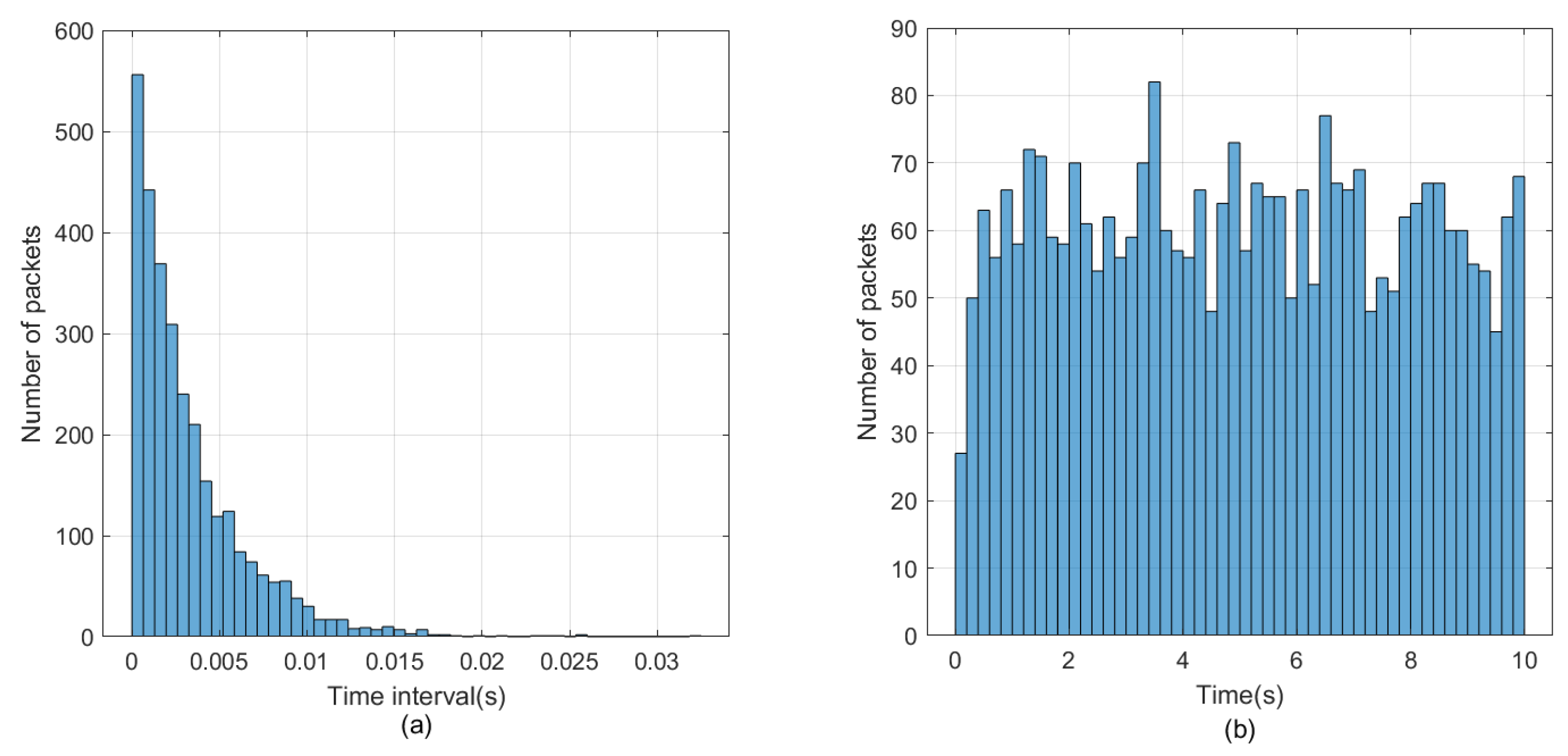
For training purpose, we built six traffic intensity models ranging from 20% to 125%. The traffic intensity is reflected as the time interval between packet generation.
Figure 6 shows the traffic model when the traffic intensity is 125%.
Figure 6a shows the time interval distribution of data packets, and
Figure 6b shows the number of data packets sent.
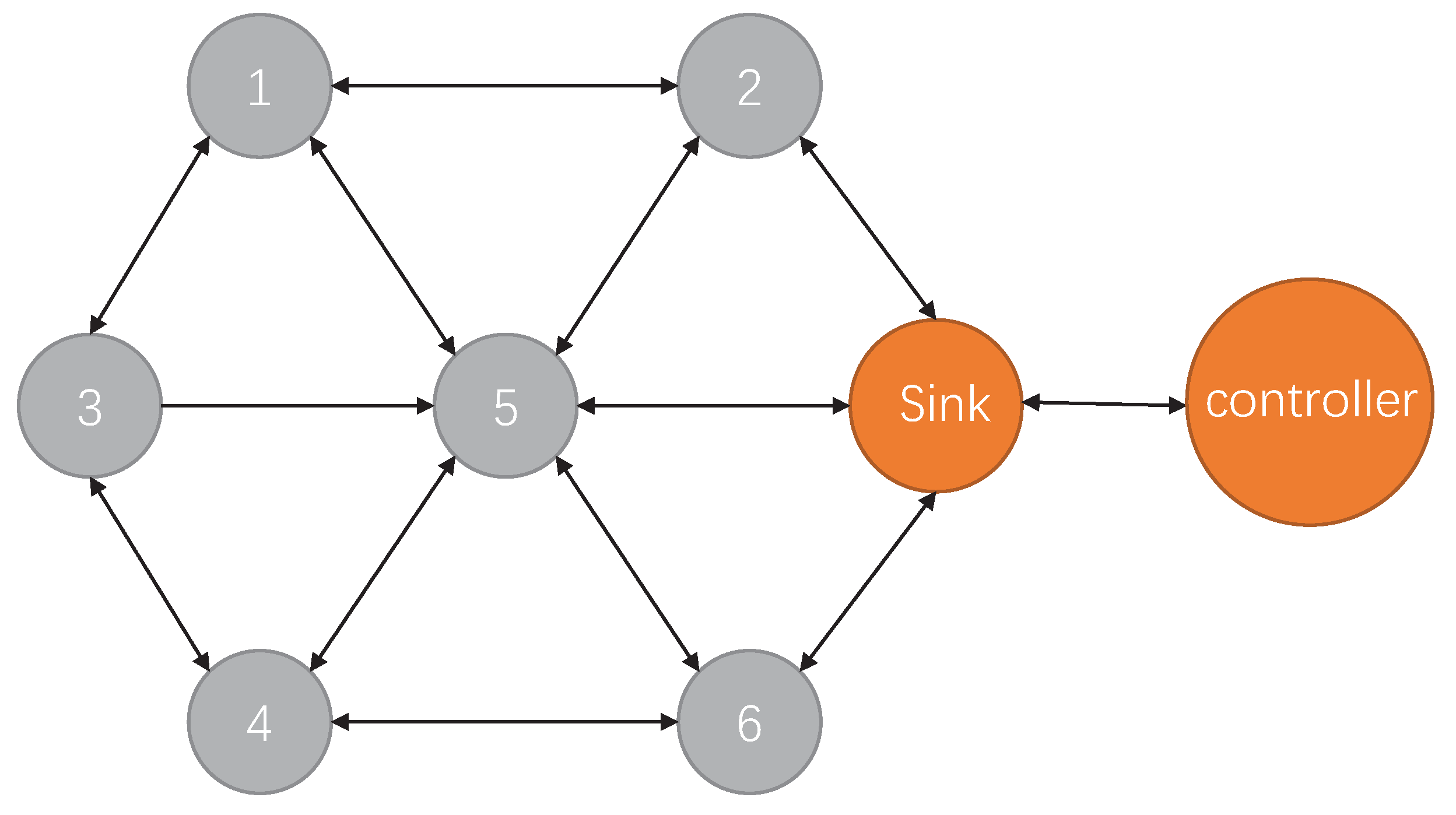
The shortest path algorithm Dijkstra is used to generate the initial packet transmission path, as well as the relevant environment data, including channel delay, packet loss rate of nodes, the occupancy of buffers, and the generated rewards value.
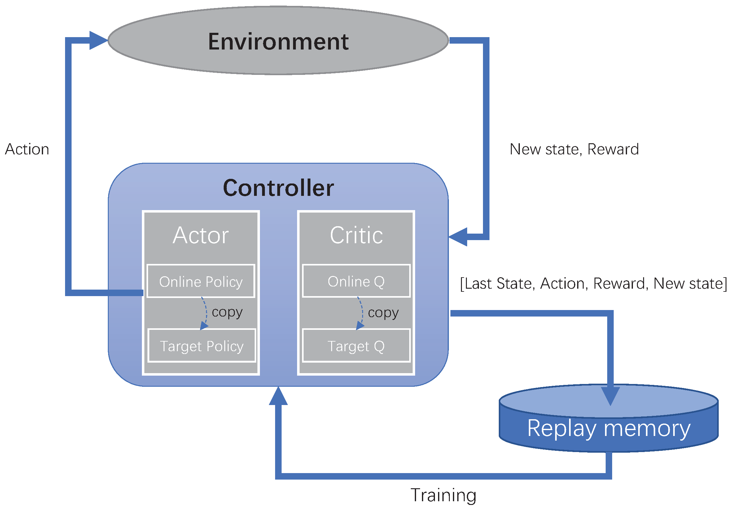
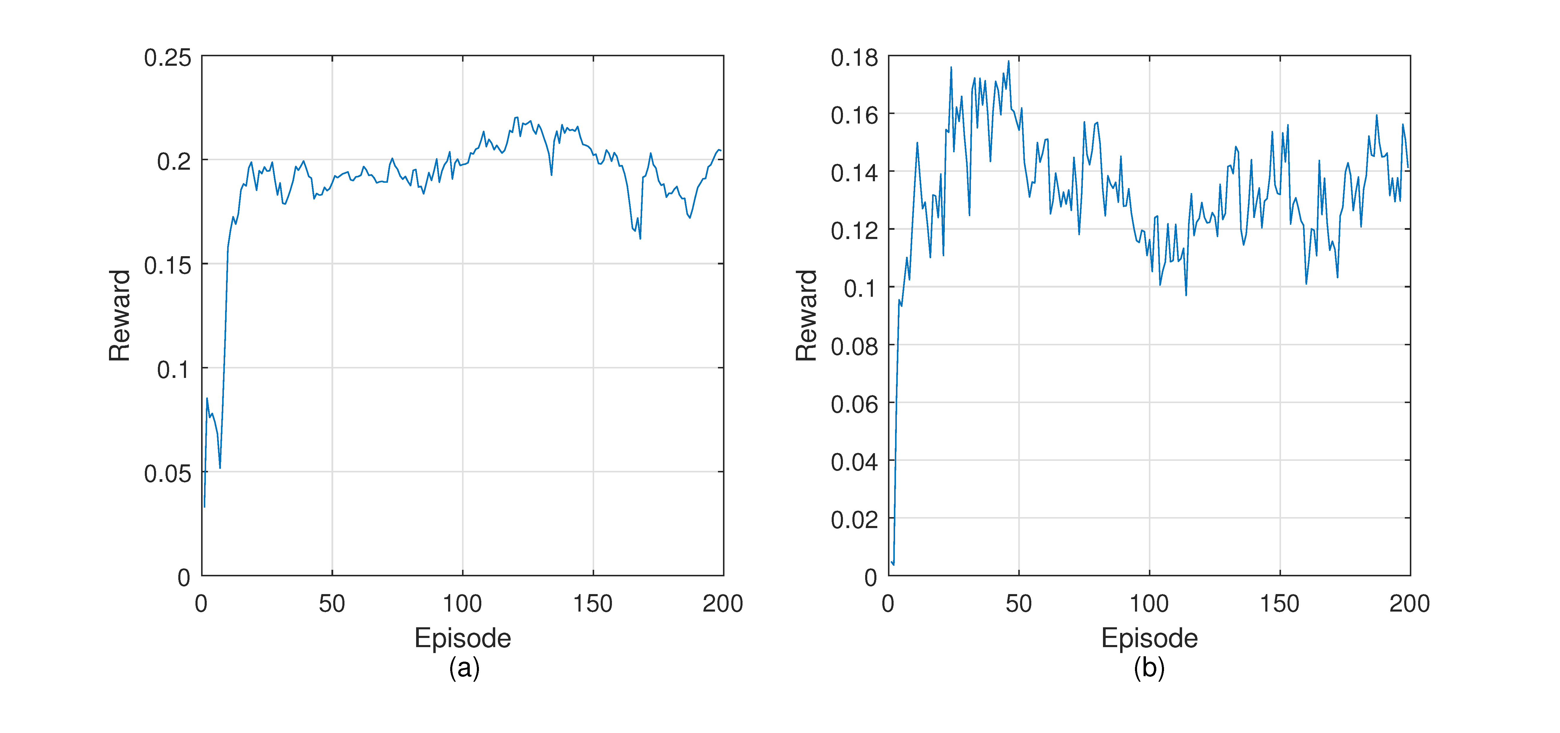
After the pre-training, the model is used to predict the transmission direction in the simulation environment. We will collect the environment data and the corresponding reward value and store them in the experience pool. The weights of all the neural networks in the model will be updated by experience playback and gradient descent. The loop will be repeated 200 times, each of which comprises 100 steps.
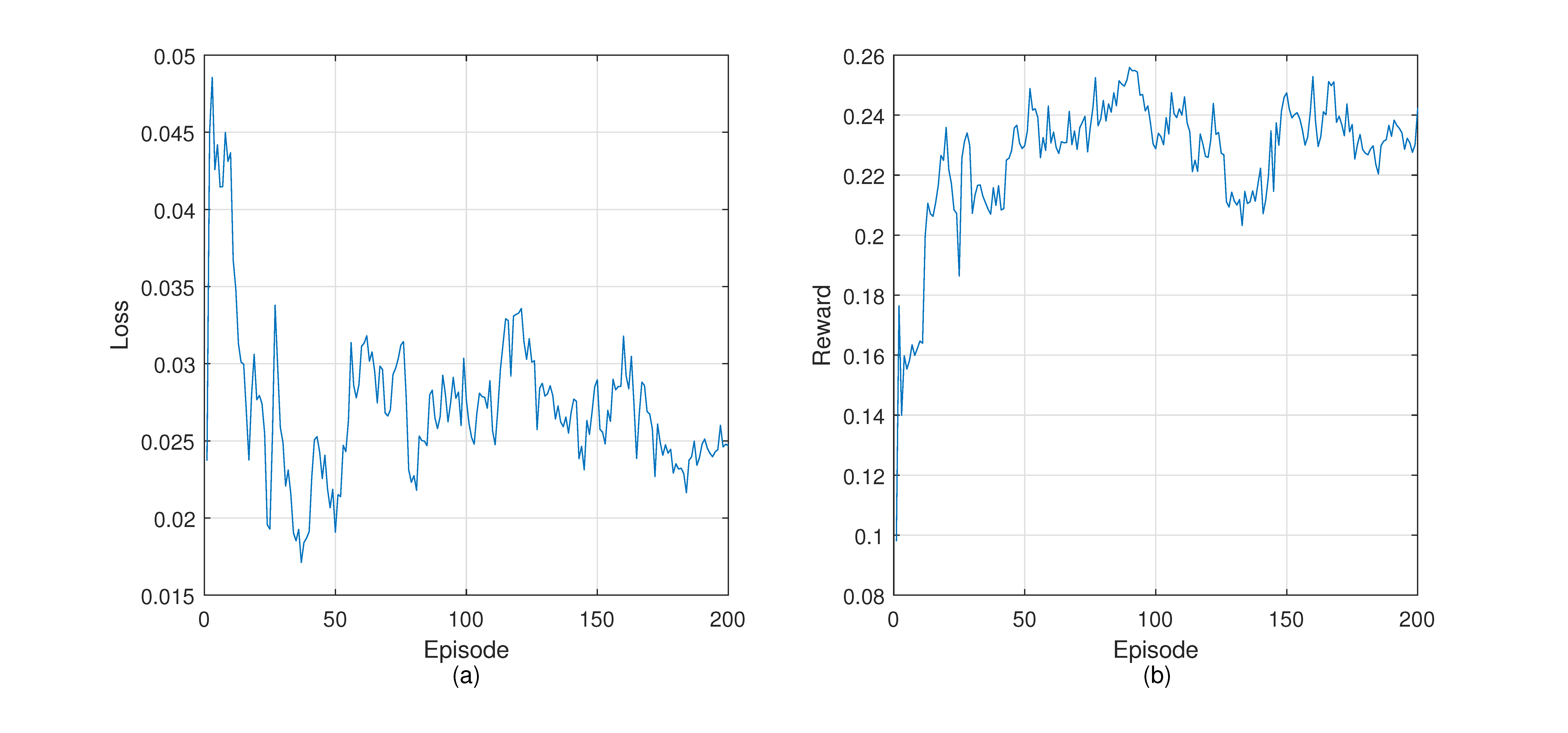
Figure 7 shows the loss and reward during the training process. The loss curve shows a downward trend on the whole. However, the loss often increases throughout the training. This can be explained by the difference between reinforcement learning and supervised learning based on fixed data sets. The training data of reinforcement learning come from the experience pool, and the data in the experience pool are collected from the environment, so they are in constant change. The loss curve fluctuates when encountering a new state space that leads to better reward. In the beginning, the reward is lower because the controller does not have enough knowledge about the network and explores the environment. After some training episodes, the reward increases rapidly. It reflects that routing policies made by the controller are able to guide packets forwarding to obtain better returns.
4.5. Evaluation Results
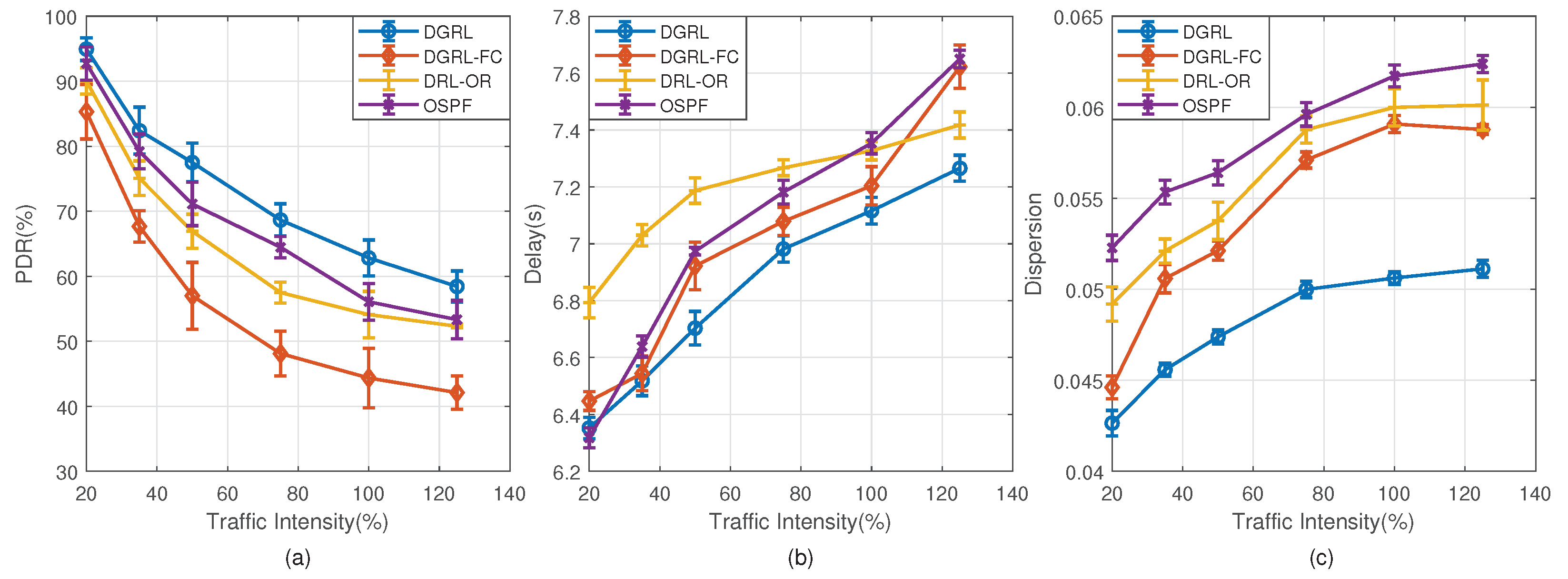
Figure 8 reflects the performance of DGRL and the three comparison algorithms under different traffic intensity. The numbers on the
x-axis are the number of traffic intensity, while the numbers on the
y-axis are the number of PDR, transmission delay, and load dispersion, respectively.
Figure 8a describes the packet delivery rate. For limited buffer, the increase of traffic intensity is prone to packet loss, which reduces the delivery rate and makes the network difficult to operate properly. Reinforcement learning helps DGRL select better routes and increase packet arrival through environmental data. As you can see from
Figure 8a, DGRL has a better delivery rate than other algorithms. Under the traffic intensity 125%, the PDR of DGRL is 5.1% higher than OSPF on average. The performance of DRL-OR is close to OSPF. From traffic intensity 75%, the PDR of DGRL-FC is less than 50%, while we notice that the PDR of others can be maintained above 50%.
Figure 8b shows the average transmission delay for four different algorithms. Each port of each node has a buffer of length 32. If the channel is free, the packets will be sent out immediately. Otherwise, they will be stored in the buffer and queue for being sent out. In this experiment, the transmission delay of data packets mainly comes from the time they queue for forwarding in the node buffer. Under low traffic intensity, the average delay of each algorithm is similar. That is because the buffers are still free, and the waiting time required for forwarding is also short. When the traffic intensity increases, the buffer occupancy rises and even the buffers are filled up. In this case, more time will be spent through this node and even packet loss will occur. OSPF considers only the shortest path, so the forwarding path is fixed. Based on the smallest number of hops, the forwarding is efficient at low traffic intensity. Under the traffic intensity 20%, it has the best performance compared with other algorithms. From traffic intensity 100%, its delay turns out to be the worst. DGRL-FC is similar to DGRL in that it considers the features of nodes, but it lacks consideration of the relationship between nodes and its neighbors. In the case of high traffic intensity, the optimization effect is poor. DRL-OR takes the traffic characteristics into consideration, alleviates congestion, and reduces delay to a certain extent. However, its delay is higher than others when the traffic intensity is low. Different from other algorithms, DGRL considers multiple factors in routing decisions, including hops and buffer occupancy. It is able to adjust the forwarding route flexibly. Under low traffic intensity, it forwards packets according to the hops. When the traffic intensity increases, buffer occupancy will play a more critical role in routing decisions.
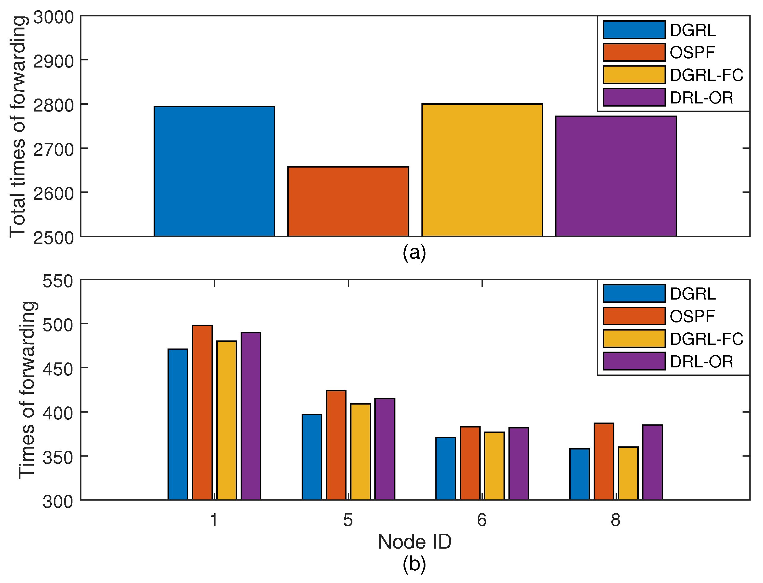
Figure 8c shows the dispersion of network load. In this experiment, the source and destination nodes of data packets are both random. Therefore, the difference of network load dispersion comes from routing. It is apparent that the network using DGRL has the smallest dispersion, while the network using OSPF has the largest dispersion. For example, under the traffic intensity 125%, the dispersion of load in network using DGRL is 0.051, whereas those of OSPF, DRL-OC, and DGRL-FC are 0.062, 0.060, and 0.058, respectively. These results confirm DGRL’s effectiveness in adjusting network load. The reasons behind lower dispersion are as follows. DGRL is an algorithm with memory. It will learn from the experience. Suppose that in a state
s, the action
a forwards the packet to a next hop whose buffer occupancy is high. The reward of this action will be low. When it is in the state
s again, it remembers that
contributes to a higher reward than
a. Therefore, it avoids forwarding packets to high occupancy nodes. In the model using OSPF, some nodes are on the shortest path of multiple source-destination nodes pairs. These nodes will bear more forwarding than edge nodes. The situation is more serious with the increase of traffic intensity.
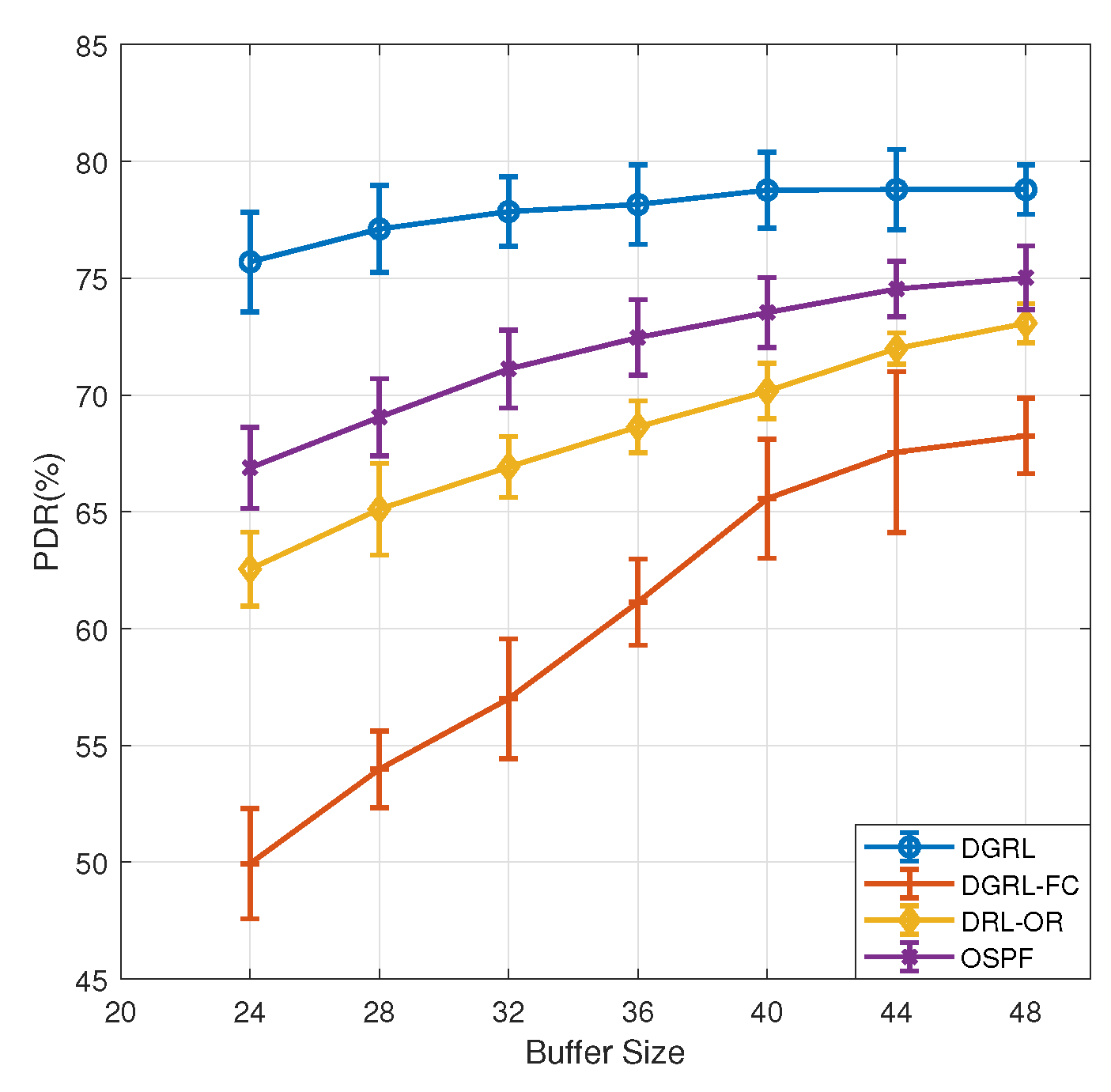
In our experiments, the new received packets will be dropped when the buffer is full. PDR is the most direct index to reflect packet loss. We designed a new experiment to verify the relationship between PDR and buffer size. The traffic intensity is fixed at 50% and the buffer size ranges from 24 to 48.
Figure 9 shows the PDR curves of each model. As we can see from the figure, buffer size has little effect on DGRL. When the buffer size is 32, as set in the previous experiments, the PDR of DGRL is 77.9%. When the buffer size is reduced to 28 and 24, the PDR decreased by 0.7% and 1.4%, respectively. When the buffer size increases to 48, the increase of PDR is little. This can be understood as DGRL has a better utilization rate for the network buffers. A buffer of size 32 already meets the requirements of DGRL. The PDR of the other three models are closely related to buffer size. As buffer size decreases from 32 to 24, the PDR of OSPF decreases by 4.2%, DRL-OR by 4.4%, and DRL-FC by 7.1%. Increasing buffer size to 48 gives a improvement, ranging from 3.9% to 11% for the three models. It is obviously due to the increase in buffer size, which reduces packet loss caused by full buffer.
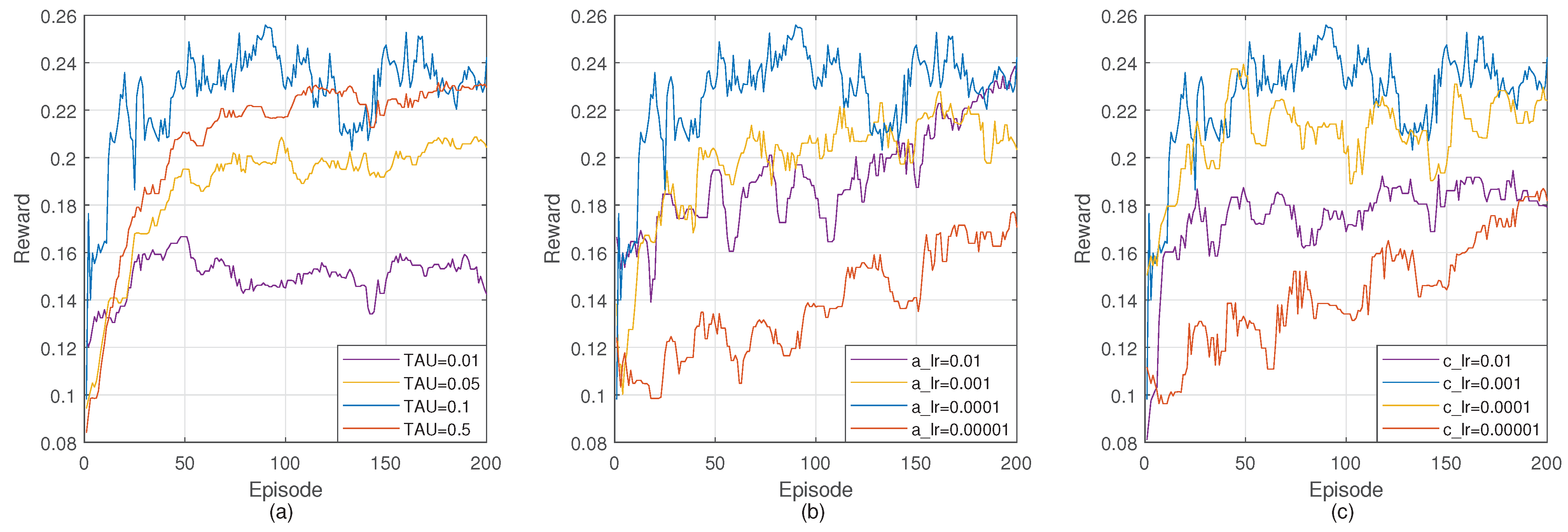
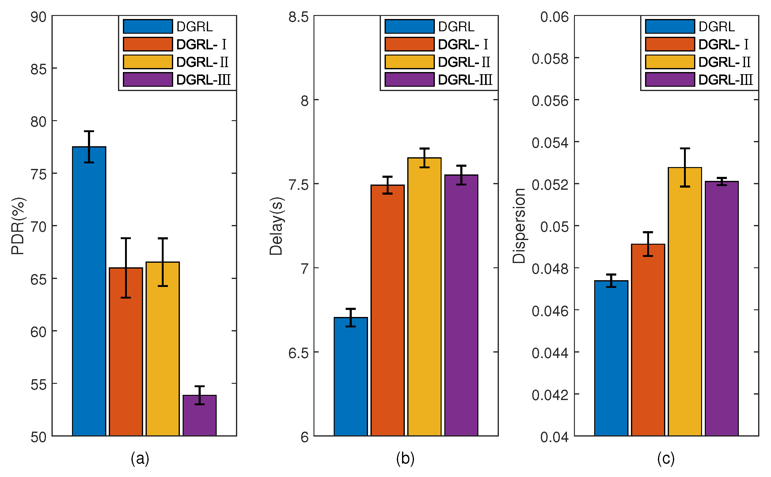
Figure 10 shows the experiment about
, which aims to reflect the influence of different parameters in the
on the training model. In this experiment, the traffic intensity is fixed at 50%. In addition to the trained DGRL model, there are three other variants of DGRL. The
function of DGRL-I considers
and
. DGRL-II considers
and
. DGRL-III considers
and
. It is clear that the performance of DGRL is better than the other three models.
Figure 10a shows that the missing parameter
has the greatest impact on the PDR. It results in a 23.6% drop in PDR than DGRL. Compared with DGRL, DGRL-I and DGRL-II also have a similar decrease in PDR.
Figure 10b shows that the loss of all the three parameters each lead to an increase in mean transmission delay.
Figure 10c shows that the impact of
and
on
is greater than that of
. In conclusion, all the three parameters are indispensable to
.


