Abstract
Automatic road extraction from unmanned aerial vehicle (UAV) imagery has been one of the major research topics in the area of remote sensing analysis due to its importance in a wide range of applications such as urban planning, road monitoring, intelligent transportation systems, and automatic road navigation. Thanks to the recent advances in Deep Learning (DL), the tedious manual segmentation of roads can be automated. However, the majority of these models are computationally heavy and, thus, are not suitable for UAV remote-sensing tasks with limited resources. To alleviate this bottleneck, we propose two lightweight models based on depthwise separable convolutions and ConvMixer inception block. Both models take the advantage of computational efficiency of depthwise separable convolutions and multi-scale processing of inception module and combine them in an encoder–decoder architecture of U-Net. Specifically, we substitute standard convolution layers used in U-Net for ConvMixer layers. Furthermore, in order to learn images on different scales, we apply ConvMixer layer into Inception module. Finally, we incorporate pathway networks along the skip connections to minimize the semantic gap between encoder and decoder. In order to validate the performance and effectiveness of the models, we adopt Massachusetts roads dataset. One incarnation of our models is able to beat the U-Net’s performance with 10× fewer parameters, and DeepLabV3’s performance with 12× fewer parameters in terms of mean intersection over union (mIoU) metric. For further validation, we have compared our models against four baselines in total and used additional metrics such as precision (P), recall (R), and F1 score.
1. Introduction
Automated road extraction remains one of the important yet challenging tasks in remote sensing imagery analysis. Its massive deployment in social and economic welfare such as city planning, road navigation, arrangement of logistic hubs, and evacuation planning makes it of great significance. However, the existence of non-road objects, occlusions, and complexity of the background make it difficult to extract roads precisely. Manually labeling the roads might be one of the methods to solve the problem, but due to its repetitious and wearisome nature, one is prone to making mistakes, let alone its inefficiency. Several methods have been proposed for extracting road information from raw UAV images. These methods can be divided into three categories: road area extraction, road centerline extraction, and road edge detection. Pixel-level segmentation of roads and their surface is the main task of road area extraction while extracting the skeleton or centerline [1] of roads is the main task of the road centerline extraction. Road edge detection [2] infers extracting single-pixel width of road edges, and it is important for autonomous driving car systems. In some studies, more than one single task is addressed simultaneously [3].
Road area extraction can be undertaken by pixel-wise semantic segmentation. Traditional road extraction methods used classic machine learning and computer vision algorithms such as support vector machines (SVM) and Markov random fields (MRF). Mie et al. (2003) used support vector machine (SVM) and template matching [4] to extract the true road segment and remove the false road segment. Jayaseeli and Mathali (2020) proposed a cuckoo search optimization algorithm for extracting road regions from high resolution images using multilevel thresholding schema and SVM [5]. Guo et al. (2011) came up with an adaptive non-planar road detection and tracking approach that combines a piecewise planar model and an MRF-based alternating optimization method [6]. Alshehhi et al. (2017) proposed an unsupervised method that consists of steps such as feature extraction (using Gabor or morphological filtering), graph-based image segmentation, and postprocessing [7]. These traditional methods include multiple steps [7], which is time consuming and requires individual optimization of each component of the model pipeline.
Currently, deep learning models have been deployed increasingly in dense classification tasks thanks to their good performance and generalization capability. Convolutional Neural Networks (CNNs) are designed to automatically and adaptively learn spatial hierarchies of features, from low to high-level patterns [8]. Fully convolutional networks (FCN) [9] for semantic segmentation by Long et al. is one of the earliest models that include only convolutional layers to extract the segmentation map. The authors modified models such as VGG16 [10] and Inception [11] networks that performed well in the object recognition domain so that the models can accept arbitrarily sized images. The fully connected layers of the models were substituted for convolution layers that upsample the extracted feature map to the same size as the input. However, due to the jump structure of the network, the fine-grained spatial information of images is lost in the upsampling process. DeConvNet [12] by Noh et al. was introduced to tackle this bottleneck by using encoder–decoder architecture. The model also adopts VGG16 network as an encoder to extract high-level feature maps. However, unlike the FCN network, the segmentation map extraction task is performed by multilayer decoder part that upsamples the output of encoder by deconvolution method (also known as transposed convolution). Badrinarayanan et al. proposed SegNet model [13], also based on encoder–decoder architecture. However, in SegNet model, the upsampling task in the decoder is performed by using pooling indices computed in the max-pooling operation executed in the encoder part. Due to the repeated implementation of max-pooling operation in the encoder part, these models suffer from a severe loss of spatial information.
In the dilated (also known as “atrous”) convolution models, dilated convolutional layers are utilized instead of using the max-pooling operation to address the spatial information loss problem. DeepLab families [14] are some of the most popular models that incorporate dilated convolutions in their architectures. Specifically, the DeepLabV3 model [15] by Chen et al. is based on three key hallmarks: first is the application of atrous convolution layers, second is the implementation of Atrous Spatial Pyramid Pooling (ASPP) that enables the input image at multiple scales, and, finally, the last is the combination of CNN methods such as VGG16 or Inception models with probabilistic graphical models to capture object boundaries.
Meanwhile, in the realm of medical image processing, a U-Net model [16] by Ronneberger et al. was proposed to segment biological microscopy images. The U-shaped model adopting an encoder–decoder structure consists of four encoding and four decoding stages and a bridge block that connects them. One of the salient features of the U-Net model is the introduction of skip connections that enable the model to retrieve any spatial information lost during pooling operations in the encoder. Since then, there have been numerous variations of the model for tackling different domain segmentation tasks [17,18,19,20,21].
In the area of deep learning-based road extraction from UAV imagery, one of the pioneering studies to utilize Deep neural networks was carried out by Mnih et al. [22]. They proposed a model based on restricted Boltzmann machines (RBMs) [23] to extract road information from UAV imagery. Their method included preprocessing and postprocessing steps. Preprocessing was applied to reduce the high dimensionality of high resolution of input images and postprocessing was deployed to polish up the disconnected parts of the predicted roads. The method proposed by [24] was fully based on Convolutional Neural Networks (CNNs) and the authors used model averaging displacement method to overcome overfitting during the inference time. Inspired by successful implementation of U-Net model into medical image processing, Zhang et al. proposed Residual U-Net [17] for extracting road information from remote sensing images. The authors injected the property of residual units within encoder–decoder stages into the classic U-net architecture to improve performance. Furthermore, Buslaev et al. proposed a network based on ResNet-34 pretrained on ImageNet-1000 dataset and a decoder adapted from vanilla U-Net model [25]. In addition, to improve performance, the authors used test-time augmentation techniques. Cheng et al. introduced CasNet, which consists of two networks: one for road detection task and the other is for obtaining centerline detection [3]. During the inference time, a thinning algorithm was proposed to obtain smooth and complete road centerline. RoadNet proposed by Liu et al. simultaneously deals with three tasks: road surface segmentation, road edge detection, and road centerline extraction [26].
Although most of the aforementioned deep learning-based models for the road extraction from the UAV imagery perform well due to their high computational complexities, these models are still too heavy to be implemented or deployed in practice on resource-constrained UAVs. The computing capacities of edge modules installed on UAVs are considered weaker than the computational capability of most deep learning platforms. AI edge modules, such as Nvidia Jetson TX2 and Jetson Nano, are some of the modules used for drones, and their computational capability is constrained compared to GPU machines used for deep learning platforms. The heaviness or lightness of networks refer to the number of parameters and the number of floating point operations of the network. The greater the number of parameters, the larger the size of the model, which makes it difficult to deploy on machines with constrained computational capability. In this paper, we aim to address this critical issue by proposing two light-weight models based on Inception module [11], ConvMixer layer, and separable depthwise convolutions. To our best knowledge, this is the first paper that combines the aforementioned modules and techniques in a single network. Both of the models contain remarkably less parameters than the baselines while achieving state-of-the-art performance on widely adopted realistic dataset.
The reminder of this paper is organized as follows: Section 2 and Section 3 introduce the building blocks of the proposed models and the methodology in detail, respectively. Section 4 describes the baseline models, the dataset, and the metrics and provides the experimental results and their discussions. Section 5 concludes this paper.
2. Preliminaries
In this section, we describe some preliminaries on the main components of the proposed models.
2.1. Building Blocks
The proposed architectures combine the cores of the following previous studies:
- U-Net network architecture;
- Depthwise separable convolutions;
- ConvMixer layer;
- Inception module.
2.1.1. U-Net for Biomedical Image Segmentation
As mentioned before, the U-Net model was originally proposed for biomedical image segmentation. The model consists of contracting path (encoder) that compresses the input data into low-dimensional representation and an expansive path (decoder) that decodes extracted information back to the original size. Both contracting and expansive path consist of four stages and in the middle, and there is a bridge comprising two convolution layers that connect them. At each stage of contracting path, there are two cascaded convolution layers to extract spatial features followed by a max-pooling operation that halves the resultant feature map. ReLU activation function is performed after all convolution layers. After each max-pooling operation, the filter size is doubled. On the other hand, at each stage of expansive path, before upsampling the feature maps with transposed convolution operation, the filter size is halved. After the upsampling process, the output is concatenated with the extracted feature map of the corresponding stage of the contracting path that enables conveying low-level spatial information to high-level layers. Aggregated information is convolved by two consecutive convolutions. At the last stage, following the two convolution operations, convolution is performed to generate the final output. It is important to point out that, in our implementation, we incorporate Batch Normalization layer [27] as a method to accelerate the training process, which was not used in the original implementation of U-Net as it did not exist at that time.
2.1.2. Depthwise Separable Convolutions
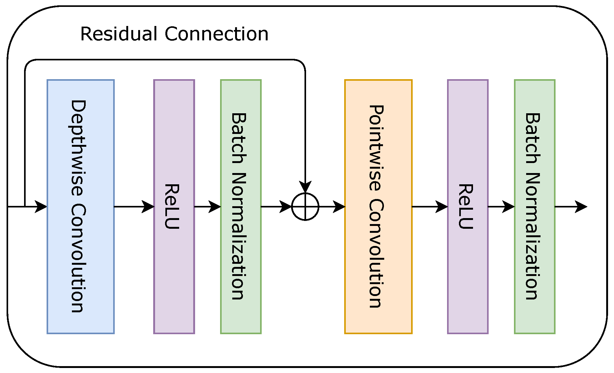
The term “depthwise separable convolutions” was used for the first time by Laurent Sifre in his PhD thesis [28]. In traditional convolutional layers, the weights in the network are shared, feature extraction and feature fusion are performed simultaneously, the invariant function is used to sample the pooling layer spatially, and a large number of parameters are generated [29]. Contrarily, depthwise separable convolutions (also known as depthwise convolutions, not to be confused with the spatially separable convolutions in the image processing community) consists of two consecutive independent convolutional layers: depthwise convolution that applies a single filter across each channel (n different filters for n-channel input) of input data and pointwise convolution- convolution that projects the output of the depthwise convolution into a new channel space [30] (see Figure 1).
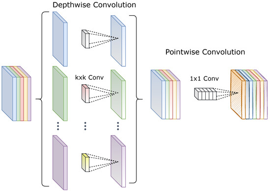
Figure 1.
Depthwise separable convolutions.
This factorization operation enables decreasing the model size and computational cost remarkably. The following includes the mathematical expressions of traditional convolution (Equation (1)), depthwise convolution (Equation (2), ⊙ denotes the element-wise product), pointwise convolution (Equation (3)), and depthwise separable convolution (Equation (4)) operations:
where W stands for the input data, y denotes convolutional filter with the size of in the case of traditional and depthwise convolution, and in the case of pointwise convolution. M and represent channel size and pixels of the input data accordingly. In order to enlighten the impact of depthwise separable convolutions, we compute the computational cost required for a traditional convolution and a depthwise separable convolution and compared them. By convolving a -shaped input data through a traditional convolution layer, we obtain a -shaped feature map where P is a spatial resolution of input data, M is the number of channels of the input or equivalently, the number of the convolution kernel, K is the filter size, Q represents the spatial resolution of the output, and N is the number of channels of the convolved feature map. Assuming that the stride is 1 and there is no padding operation, the computational cost of the standard convolution is as follows.
In the case of depthwise separable convolutions, depthwise convolution operation is performed first. The cost of depthwise convolution is given by the following.
Next, the pointwise convolution is performed, which results in the following.
In total, depthwise separable convolution operation yields the following.
By factorizing the standard convolution into two parts, computational cost can be reduced by the following.
Applications of depthwise separable convolutions can be found in the Xception model [30] by Francois Chollet and MobileNet family [31,32,33] by Howard et al. and Sandler et al. In one incarnation of their MobileNets model, Howard et al. [31] were able to successfully decrease the parameter size up to 4.2 million while attaining a decent 70.6% Top 1 accuracy on ImageNet-1000 [34] dataset. For comparison, the VGG16 model with 138 million parameters achieved 71.5% accuracy [31] on the same task.
2.1.3. ConvMixer Layer
Recently, [35] proposed a novel architecture based on depthwise separable convolutions for the object recognition task. The architecture is inspired by the mixing idea [35] of the MLP-Mixer model [36] by Tolstikhin et al. Specifically, depthwise convolution serves as a tool to mix spatial locations followed by a pointwise convolution that mixes channel locations. Figure 2 highlights the modified version of the original ConvMixer layer, which is used in our ConvMixer Inception Block (see Section 2.1.4). The difference from the original version is that the orders of Batch normalization [27] operation and activation layers are swapped. In addition, we use the ReLU [37] activation function for all layers instead of GELU [38].
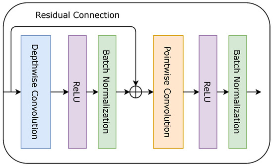
Figure 2.
The architecture of the ConvMixer layer (CML) that substitutes standard convolutional layers in the proposed ConvMixer inception block. Here, ⨁ stands for the element-wise addition of the input and the output of the Depthwise convolution followed by the ReLU activation function and Batch normalization.
2.1.4. ConvMixer Inception Block
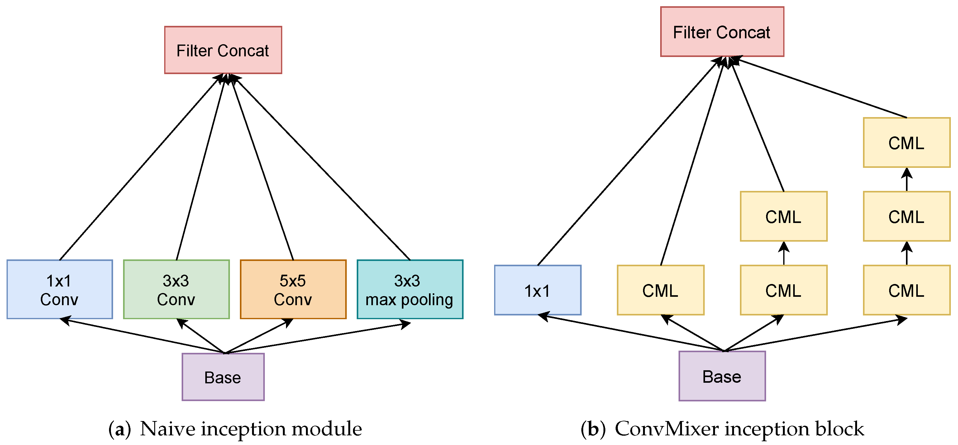
The Inception module [11] is one of the ground-breaking architectures in the deep learning realm. Prior studies built deeper networks by stacking convolutional layers on top of each other to achieve superior performance. However, the larger and deeper the model becomes, the more prone it is to overfitting and vanishing gradients [39]. On top of that, the increase in model size results in an increase in computational cost as well. The inception network was designed to overcome these obstacles. Another important aspect of this architecture is that it allows the model to learn the input image at different scales simultaneously. Figure 3a illustrates the naive inception module. The input (base) proceeds through , , convolutions, and max-pooling independently, and the outputs are concatenated to be used as an input to the next layer.
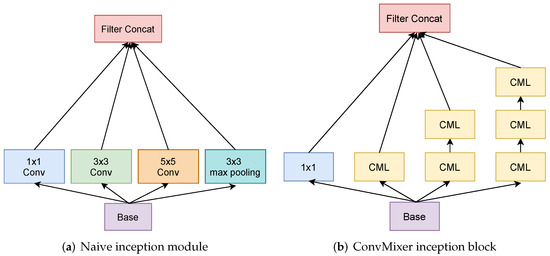
Figure 3.
Comparison of naive inception module (a) and the proposed ConvMixer inception block (b). Note that and convolutions are expressed by two and three stacked ConvMixer layers (CML), respectively, in the proposed ConvMixer inception block (b).
Furthermore, in their updated inception-v2 and inception-v3 versions [40], the authors incorporated several upgrades to the inception module, which resulted in a boost in performance and a remarkable reduction in model size. Specifically, one of the important changes was to factorize convolution operation into two convolutions since two stacked convolutions produce the same effect of a single convolution for a reduced cost of computation. We leveraged this idea in designing our architectures. However, instead of using standard convolutions, we adopt ConvMixer layers (see Figure 3b) with filter size to learn image features. In addition, we replaced the max-pooling operation with standard convolution. Following [40], and convolutions are represented by a series of two and three ConvMixer layers accordingly. In the original implementation, the ratio of , convolutions, and max-pooling layer within a module increases as it becomes deeper. However, for the sake of simplicity, we keep it equal for all filter sizes across the entire model. The method for building the network architectures of the proposed models is explained in detail in the next section.
3. Proposed Model Architectures
In this study, we propose two light-weight models based on U-Net, inception module, ConvMixer layer, and depthwise separable convolutions.
3.1. Mixer U-Net
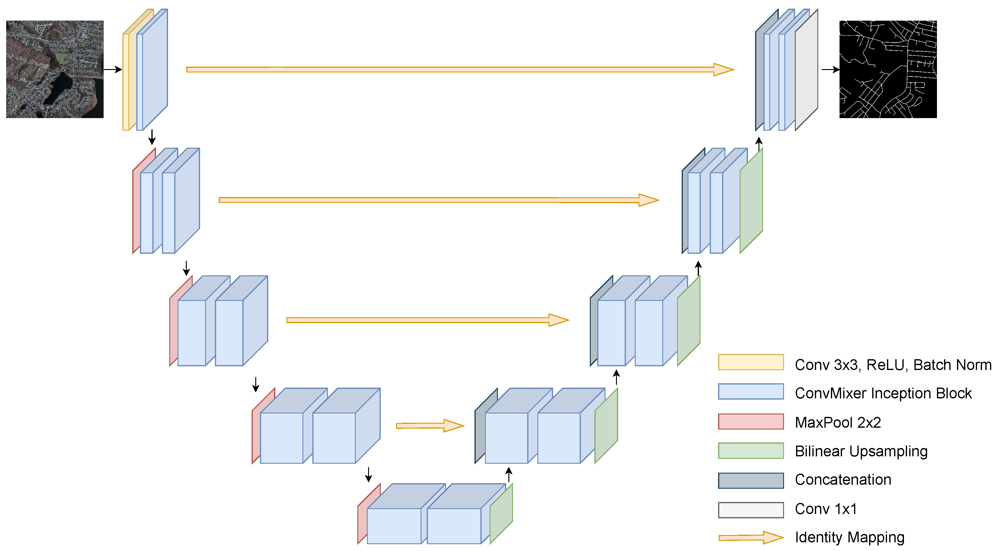
Figure 4 illustrates the methodology of the first proposed model, namely, the mixer U-Net. The model adopts the U-shaped structure of the U-Net model consisting of four encoding and decoding stages with a bridge that connects them. As mentioned in Section 2.1.4, unlike in the U-Net, in the proposed mixer U-Net, all standard convolutions are replaced with ConvMixer inception block except the first encoding stage. Thus, it is called Mixer U-Net. At the first stage, the input proceeds through an embedding layer, which is a standard convolution followed by a ConvMixer inception block. At each of the next stages of encoder, the resolution of the input is, first, halved by the max-pooling operation and then convolved by two ConvMixer inception blocks. The number of feature channels, as in U-Net, increases from 64 at the first stage of the encoder and eventually reaches 1024 at the bridge. It should be noted that the resolution of the input image should be divisible by 16 as it is downsampled by two at each stage with 16-times in total by the time it hits the bridge.
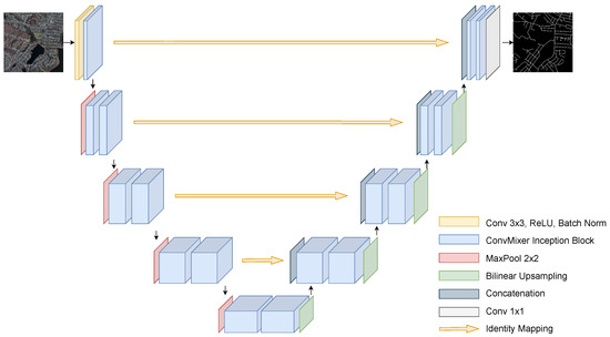
Figure 4.
The architecture of the proposed Mixer U-Net.
In the U-Net model, the feature maps are upsampled by the transposed convolution (also known as deconvolution) operation [12]. However, there are two bottlenecks in using this method. First of all, as the transposed convolution is also a convolution operation that maps lower resolution input into higher resolution output, it has learnable parameters, which means additional computational cost. On top of that, it can result in “uneven overlap” in some pixels of the upsampled feature map or so-called “checkerboard artifact” [41,42]. In order to avoid these effects caused by the deconvolution operation, the bilinear interpolation method is exploited in the proposed mixer U-Net. Thus, at the end of every stage of decoder, including the bridge, the extracted feature map is upsampled with bilinear interpolation before concatenating it with the output of the mirroring encoder stage. Next, the concatenated feature map is convolved with two ConvMixer inception blocks. At the final stage, after convolution operations, convolution is used for extracting the binary segmentation map.
3.2. Mixer U-Net with Path Networks
It is well-known that the lower-level layers of convolutional neural networks learn low-level features such as edges, blobs, or corners [43]. Moreover, as it becomes deeper, the features become more class-specific such as parts of objects in the image or an entire object as a whole. In our model, there are skip connections at each stage of encoder that enable the model to convey spatial information to the mirroring decoder stage. However, comparatively raw feature map of the first stage of encoder gets concatenated with well-processed high-level input feature map of the last decoder stage. This mismatch between the two array of features becomes lower as we move forward along the model. This semantic gap between the two sets might result in an inferior performance [19]. Hence, in order to lessen the divergence between encoder and decoder feature maps, we propose our second architecture that is an updated version of the first proposed model additionally with path networks along the skip connections (see Figure 5). At the first stage of encoder, the extracted feature map is passed on through four ConvMixer layers before being concatenated with the corresponding stage input. It is important to point out that the resolution and the number of channels remain the same throughout the entire network. As the model becomes deeper, the number of layers of the path network is reduced by one, leaving a single layer at the fourth stage. Everything else is processed consistently with the previous architecture. In the next section, the superiority and effectiveness of the two proposed models are demonstrated by conducting extensive experiments.
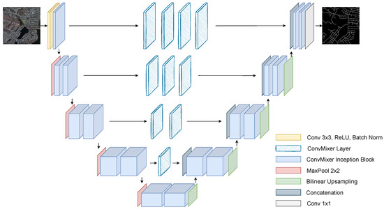
Figure 5.
The architecture of the proposed Mixer U-Net with Path Networks (PN).
4. Experiments, Results and Discussion
4.1. The Dataset and Preprocessing
Figure 6 highlights the flowchart of methodologies used in this paper. In order to evaluate the performance of the proposed models, we use publicly available Massachusetts Roads dataset [44] for the experiments. The dataset consists of 1171 aerial images covering over 2600 square kilometers of urban, suburban, and rural areas of the state of Massachusetts, USA. The dataset is randomly split into 1108 images for training, 14 images for validation, and 49 images for testing. The spatial resolution of all images is pixels covering an area of 2.25 square kilometers per image. The dataset is considered one of the largest and challenging road detection datasets available.
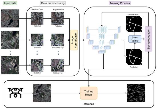
Figure 6.
The flowchart of methodologies.
Before training the model, we preprocess the data as follows. As the spatial size of images is too large for training, we crop images randomly to . Then, we apply randomly one of the horizontal flip, vertical flip, or 90 rotation augmentation techniques to introduce some randomness into the dataset. Finally, we normalize the images with the mean and standard deviation of the entire dataset. During the inference time, the image is resized to as the models accept only images with the size divisible by 16. After that, it is normalized with the mean and standard deviation of the training set. The additional padded two pixels on each side of the image are discarded during the evaluation.
4.2. Implementation Details
The proposed models, along with the baselines, were implemented on Python 3.8.12 and Pytorch 1.10. The experiments were performed on a single NVIDIA RTX A5000 GPU with 24 GB memory. An Adam optimizer was used to optimize the models with the initial learning rate set to 0.001. Cosine Annealing learning rate scheduler [45] is applied to control the learning rate during training. All models were trained for 200 epochs with mini-batch size equal to 8.
Binary Cross Entropy (BCE) (Equation (10)) loss is considered to be stable and works best in the case of equal class distribution [46]. However, our dataset suffers severely from class imbalance. In this case, Dice loss (Equation (11)) is preferred as it does not treat every pixel individually but measures the overlap between two samples. By leveraging the stability of BCE loss and flexibility of Dice loss of class imbalance, we can adopt a Combo loss (Equation (12)) that is the combination of two loss functions [46,47].
In Equation (11), a smooth (usually set to 1) variable is added in both the numerator and denominator to ensure that, in the case of , the function is not undefined.
4.3. Baseline Models
We compare the performance of the proposed models against four state-of-the-art deep learning-based models, specifically, Fully Convolutional Networks (FCN) [9], U-Net [16], ResU-Net [17], and DeepLabV3 [15]. FCN is considered as a milestone in deep-learning based semantic segmentation models. In addition, FCN is one of the first models built on only convolutional layers in the semantic segmentation domain. Although U-Net was originally proposed for medical image processing, several variations of it were successfully deployed in different domains. In addition to that, both of our models are built based on U-Net architecture. Thus, comparing the proposed models’ performance against U-Net and FCN would be appropriate. Furthermore, ResU-Net is one of the variations of U-Net implemented in the realm of road detection from remote sensing imagery. On top of that, the parameter size of ResU-Net is relatively smaller than other baselines. Finally, DeepLabV3 is one of the recently developed networks in the general semantic segmentation research area, and it would be interesting to check the performance of this model on the binary segmentation task that we are dealing with in this study. It should be noted that the backbone network of both DeepLabV3 and FCN is ResNet50 pretrained on ImageNet-1000 dataset [34]. All baseline models were trained from scratch with the same parameters used in the training of the proposed models.
4.4. Evaluation Metrics
Some of the common evaluation metrics for semantic segmentation are pixel accuracy (PA), Precision, Recall, F1 score, and Jaccard index. However, as mentioned above, the Massachusetts roads dataset suffers from a severe class imbalance problem, i.e., the number of pixels representing the background exceeds the number of pixels denoting road areas excessively. Thus, using a pixel accuracy metric for the purpose of evaluation would be inappropriate. The following equations are the mathematical expressions of the above-mentioned metrics, except :
where , , and stand for the number of true positive, false positive, and false negative predictions, respectively. Precision is the ratio of true positives to the prediction, while recall is the ratio of true positives to the ground truth. The F1 score is the harmonic mean of precision and recall. The Jaccard index, also known as mean intersection over union (mean IoU), is the ratio of the intersection and union for the two sets A and B. All metrics are calculated on each class separately, and their average is reported as the final score.
4.5. Results and Analysis
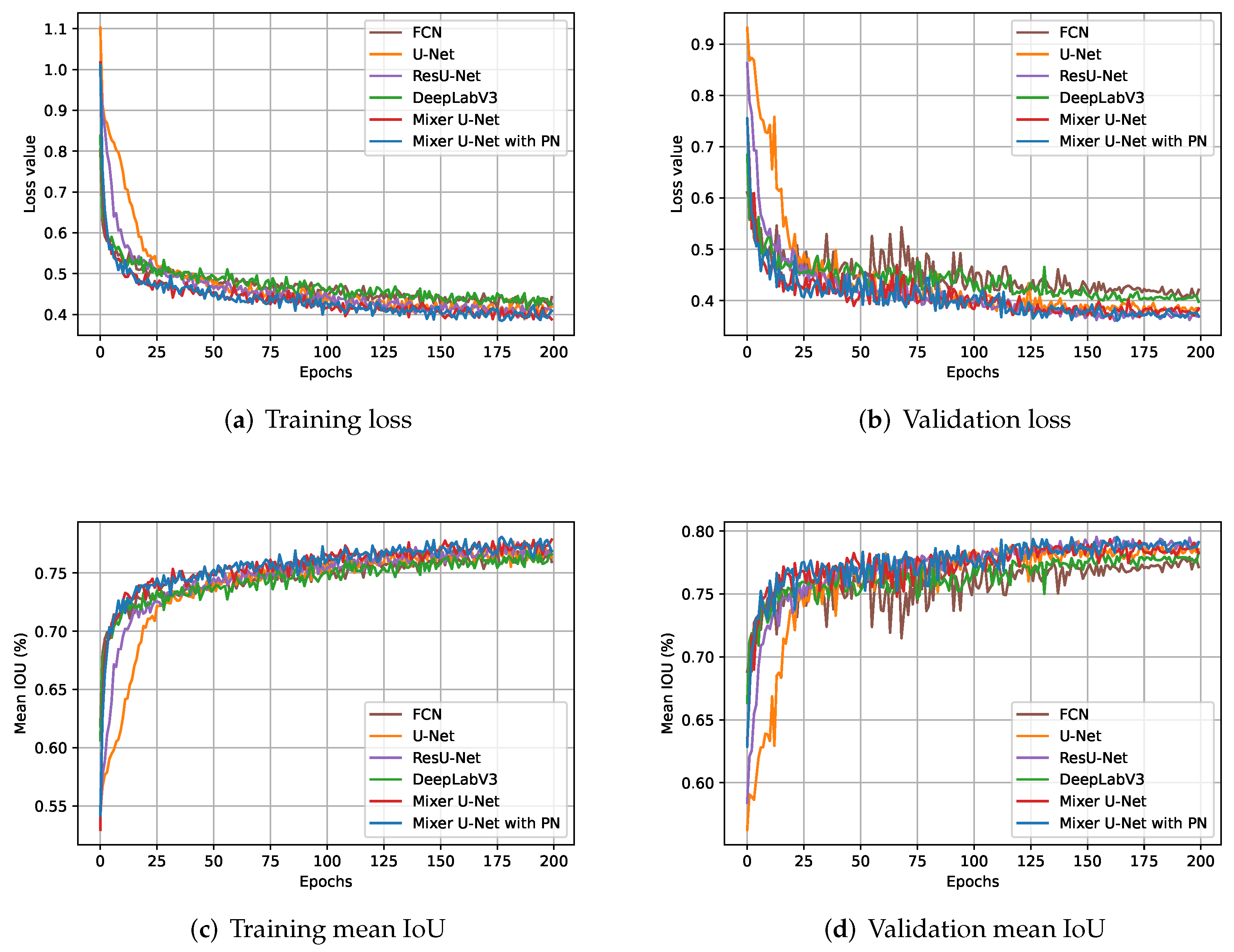
Figure 7 highlights the learning curves of all models during the training and validation process. In particular, Figure 7a,b elucidate the loss value, and Figure 7c,d portray mean IoU scores during training and validation, respectively.
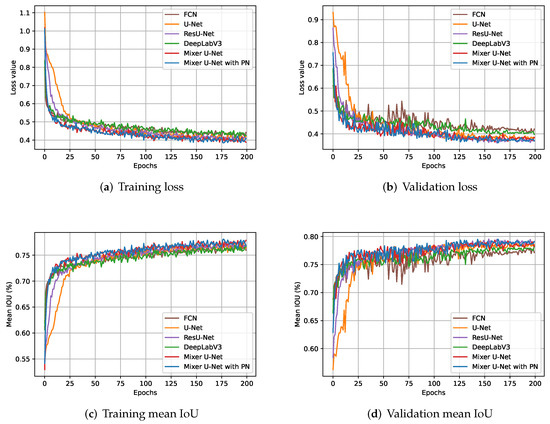
Figure 7.
Learning curves for the four baselines and the proposed models during training and validation. In all Figures, x-axis highlights the number of training epochs. In Figures (a,b), y-axis represents loss value, and in Figures (c,d), it describes the mean intersection over union (mean IoU) in percentage (%).
It can be noted from Figure 7 that U-Net and ResU-Net experience a slower convergence compared to other models while the proposed models yield the fastest convergence exceeding the 75% mean IoU benchmark easily within the first 10 epochs in the validation. However, in order to unlock the full potential of all models, we keep training them until performance is saturated. As a result, by the end of training, the proposed models remained dominant while the performance gap among models shrunk remarkably, scoring negligibly lower than 80% mIoU both on the training and validation sets.
Table 1 summarizes the quantitative results of our experiments. Evidently, all models attained competitive results across all metrics in the inference time. Despite the fact that the proposed Mixer U-Net and Mixer U-Net with PN contain roughly 10-times fewer parameters than the baselines except ResU-Net, the models achieved the highest mIoU, recall, and F1 score, losing slightly to U-Net and ResU-Net in terms of precision. Among all models, FCN and DeepLabV3 yield inferior results, most probably, due to the reason that these models’ backbone was pretrained on ImageNet-1000 dataset, the distribution of which notably differs from the target dataset. Although the ResU-Net model experiences relatively slower convergence at the beginning of the training, it achieves the highest results among the baseline models, surpassing the proposed models as well in terms of precision. It can be concluded that training models until full convergence might result in superior performance despite their initially slower convergence.

Table 1.
Quantitative results.
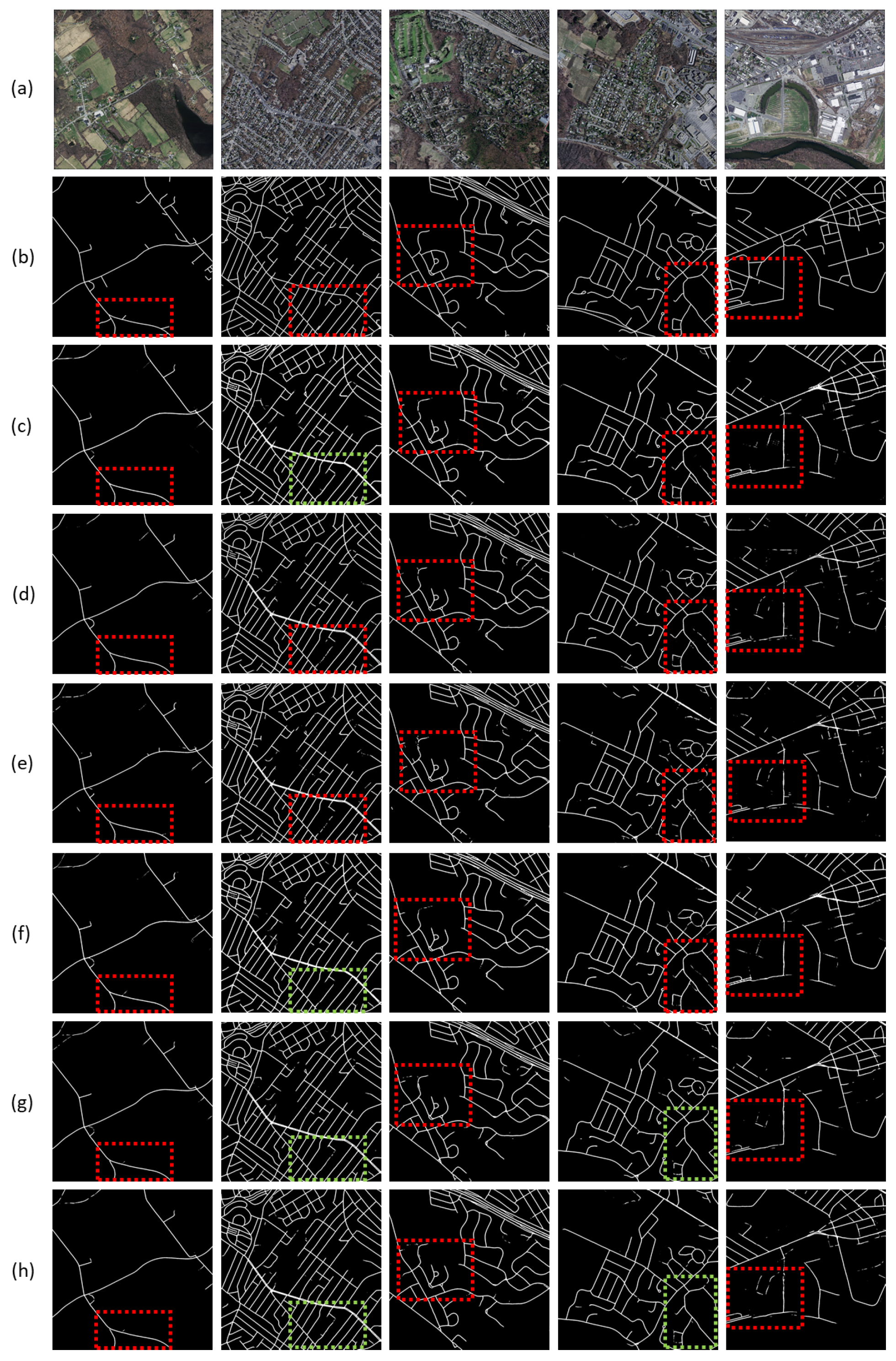
Generally, all models yield good results with small distortion or misdetection. Figure 8 illustrates segmentation maps extracted by the models. Five images (row (a)) with varying difficulty were chosen randomly from the test set. The red dotted rectangles show areas where the models struggled the most, whereas green ones represent areas with relatively improved accuracy. On the first, third, and fifth images, all models struggle on the highlighted areas. However, on the second and fourth images, the proposed models extract nearly identical segmentation maps as the ground truth.
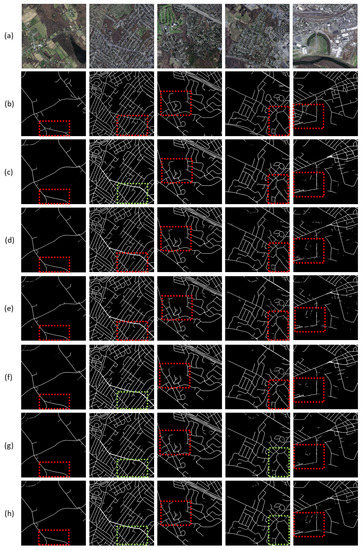
Figure 8.
Visual comparison of road extraction results by the baselines and the proposed models on randomly chosen images from the test dataset. The first two rows-(a,b) represent the original image and the ground truth, respectively. The order of models is as follows: (c) FCN, (d) U-Net, (e) ResU-Net, (f) DeepLabV3, (g) Mixer U-Net (ours), and (h) Mixer U-Net with PN (ours). Dotted red rectangles represent the areas of the image with poor performance, while dotted green rectangles highlight areas with better performance.
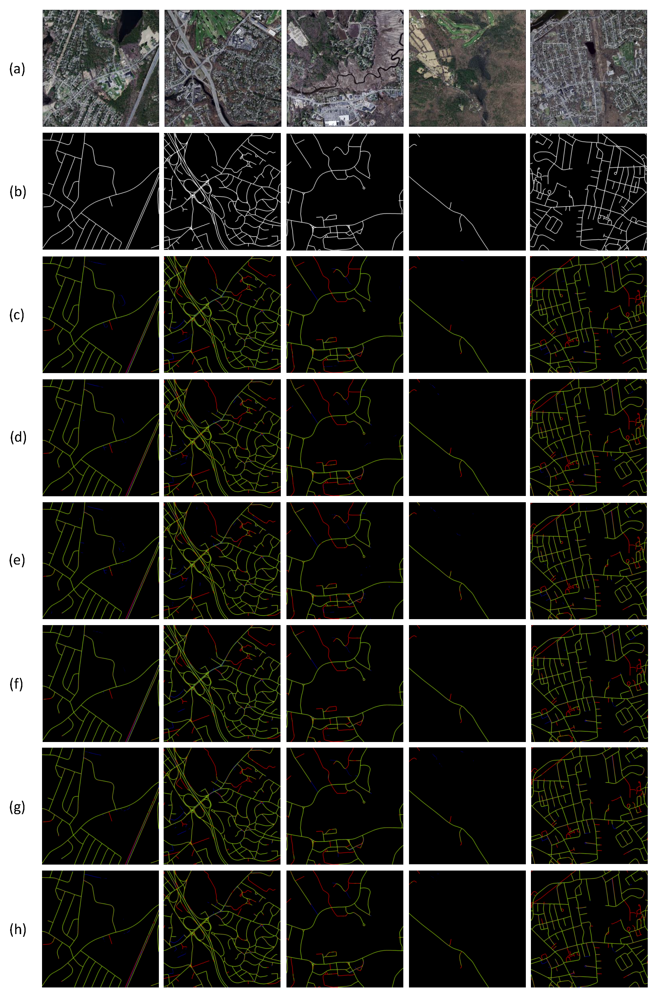
In order to further explore the areas on images where the models struggle the most and the reasons for that, we conducted an error analysis (see Figure 9). For the same goal, another set of five images was randomly chosen from the test set and the extracted segmentation maps were overlaid on top of the ground truth. The green pixels (TP) represent the accurately detected road pixels while the blue lines (FP) denote the pixels mistakenly assigned as road pixels. Finally, the red lines (FN) illustrate areas where the models could not detect the roads and classified them as the background. In general, the models can distinguish roads from areas such as building roofs, rivers, or the parts of roads occluded with trees. However, the models treat parking lots or pavements alongside buildings or houses as roads since the context information of these parts of images is similar to the structure of roads. Moreover, the models struggle with the images where roads are occluded by the shadow of buildings and the ones which are small in width and light grey. On top of that, when the images and their ground truth labels were examined thoroughly, it was detected that not all roads were labeled but were, instead, classified as the background. This might be one of the reasons why the models are struggling to perform properly on those aforementioned areas.
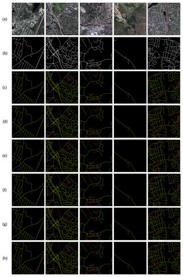
Figure 9.
Error analysis of models: visual comparison of road extraction results by the baselines and the proposed models on randomly chosen images from the test dataset. The first two rows-(a,b) represent the original image and the ground truth, respectively. The order of models is as follows: (c) FCN, (d) U-Net, (e) ResU-Net, (f) DeepLabV3, (g) Mixer U-Net (ours), and (h) MixerU-Net with PN (ours). The green, red, and blue lines represent true positives (TP), false negatives (FN), and false positives (FP) for road pixels.
5. Conclusions
In this paper, we proposed two lightweight models based on U-Net, depthwise separable convolutions, ConvMixer layer, and an inception module to extract road areas from unmanned aerial vehicle imagery. Specifically, the standard convolution operation used in naive inception block was substituted for the ConvMixer layer, which produces the same result for reduced computational cost. In addition to that, we replaced the max-pooling operation in the original inception module with three cascaded ConvMixer layers that produces the effect of one convolution operation. The utilization of the inception module allowed us to learn images on different scales. Furthermore, path networks were incorporated along skip connections to alleviate the semantic gap between encoder and decoder stages. Finally, we substituted the transposed convolution upsampling method in the decoder part of the networks for Bilinear interpolation to overcome the checkerboard artifact issue. We conducted extensive experiments on publicly available Massachusetts roads dataset. The experiments show that the proposed models yielded superior results compared to four state-of-the-art models while containing remarkably fewer parameters. On top of that, the proposed models experienced relatively faster convergence compared to baseline networks, easily achieving 75% accuracy benchmark within only 10 epochs of training.
Although the proposed models allowed us to decrease the parameter size considerably, performance was negligibly higher than that of the baseline models. We believe that there is still a room for improvement for our models not only in terms of performance but also further reductions in parameter size. One example could be the optimization of channel size distributions within the inception blocks across the models, which is set equally for all channels in this work. In future studies, we will carry on improving our models and investigate their potential by experimenting with various domain datasets.
Author Contributions
Conceptualization and methodology, F.S.; validation and formal analysis, F.S.; resources and data curation, J.-H.P.; writing—original draft preparation, F.S.; investigation, D.-W.L.; writing—review and editing, J.-M.K. and S.Y.; supervision, J.-M.K. All authors have read and agreed to the published version of the manuscript.
Funding
This research was funded by Dongil Culture and Scholarship Foundation.
Institutional Review Board Statement
Not applicable.
Informed Consent Statement
Not applicable.
Data Availability Statement
Massachusetts roads dataset can be found at https://www.cs.toronto.edu/~vmnih/data/ (accessed on 9 January 2022).
Conflicts of Interest
The authors declare no conflict of interest.
Abbreviations
The following abbreviations are used in this manuscript:
| UAV | Unmanned aerial vehicle |
| DL | Deep learning |
| CNN | Convolutional neural networks |
| SVM | Support vector machines |
| MRF | Markov random fields |
| FCN | Fully convolutional network |
| CML | ConvMixer layer |
| BCE | Binary cross entropy |
| mIoU | Mean intersection over union |
| PA | Pixel accuracy |
| TP | True positive |
| FP | False positive |
| FN | False negative |
References
- Huang, X.; Zhang, L. Road centreline extraction from high-resolution imagery based on multiscale structural features and support vector machines. Int. J. Remote Sens. 2009, 30, 1977–1987. [Google Scholar] [CrossRef]
- Li, X.; Zhang, S.; Pan, X.; Dale, P.; Cropp, R. Straight road edge detection from high-resolution remote sensing images based on the ridgelet transform with the revised parallel-beam Radon transform. Int. J. Remote Sens. 2010, 31, 5041–5059. [Google Scholar] [CrossRef] [Green Version]
- Cheng, G.; Wang, Y.; Xu, S.; Wang, H.; Xiang, S.; Pan, C. Automatic Road Detection and Centerline Extraction via Cascaded End-to-End Convolutional Neural Network. IEEE Trans. Geosci. Remote Sens. 2017, 55, 3322–3337. [Google Scholar] [CrossRef]
- Mei, T.; Li, F.; Qin, Q.; Li, D. Road extraction from remote sensing image using support vector machine. In Proceedings of the Third International Symposium on Multispectral Image Processing and Pattern Recognition, Beijing, China, 20–22 October 2003; Volume 5286, pp. 299–304. [Google Scholar] [CrossRef]
- Jayaseeli, J.D.D.; Malathi, D. An Efficient Automated Road Region Extraction from High Resolution Satellite Images using Improved Cuckoo Search with Multi-Level Thresholding Schema. Procedia Comput. Sci. 2020, 167, 1161–1170. [Google Scholar] [CrossRef]
- Guo, C.; Mita, S.; McAllester, D.A. Adaptive non-planar road detection and tracking in challenging environments using segmentation-based Markov Random Field. In Proceedings of the 2011 IEEE International Conference on Robotics and Automation, Shanghai, China, 9–13 May 2011; pp. 1172–1179. [Google Scholar]
- Alshehhi, R.; Marpu, P.R. Hierarchical graph-based segmentation for extracting road networks from high-resolution satellite images. ISPRS J. Photogramm. Remote Sens. 2017, 126, 245–260. [Google Scholar] [CrossRef]
- Yamashita, R.; Nishio, M.; Do, R.K.G.; Togashi, K. Convolutional neural networks: An overview and application in radiology. Insights Imaging 2018, 9, 611–629. [Google Scholar] [CrossRef] [Green Version]
- Long, J.; Shelhamer, E.; Darrell, T. Fully Convolutional Networks for Semantic Segmentation. In Proceedings of the IEEE Conference on Computer Vision and Pattern Recognition, Boston, MA, USA, 7–12 June 2015. [Google Scholar]
- Simonyan, K.; Zisserman, A. Very Deep Convolutional Networks for Large-Scale Image Recognition. arXiv 2014, arXiv:1409.1556. [Google Scholar]
- Szegedy, C.; Liu, W.; Jia, Y.; Sermanet, P.; Reed, S.E.; Anguelov, D.; Erhan, D.; Vanhoucke, V.; Rabinovich, A. Going Deeper with Convolutions. In Proceedings of the IEEE Conference on Computer Vision and Pattern Recognition, Boston, MA, USA, 7–12 June 2015. [Google Scholar]
- Noh, H.; Hong, S.; Han, B. Learning Deconvolution Network for Semantic Segmentation. In Proceedings of the IEEE International Conference on Computer Vision, Santiago, Chile, 7–13 December 2015. [Google Scholar]
- Badrinarayanan, V.; Kendall, A.; Cipolla, R. SegNet: A Deep Convolutional Encoder-Decoder Architecture for Image Segmentation. IEEE Trans. Pattern Anal. Mach. Intell. 2017, 39, 2481–2495. [Google Scholar] [CrossRef]
- Chen, L.C.; Papandreou, G.; Kokkinos, I.; Murphy, K.; Yuille, A.L. DeepLab: Semantic Image Segmentation with Deep Convolutional Nets, Atrous Convolution, and Fully Connected CRFs. IEEE Trans. Pattern Anal. Mach. Intell. 2017, 40, 834–848. [Google Scholar] [CrossRef] [Green Version]
- Chen, L.; Papandreou, G.; Schroff, F.; Adam, H. Rethinking Atrous Convolution for Semantic Image Segmentation. arXiv 2017, arXiv:1706.05587. [Google Scholar]
- Ronneberger, O.; Fischer, P.; Brox, T. U-Net: Convolutional Networks for Biomedical Image Segmentation. In Proceedings of the International Conference on Medical Image Computing and Computer-Assisted Intervention, Munich, Germany, 5–9 October 2015. [Google Scholar]
- Diakogiannis, F.I.; Waldner, F.; Caccetta, P.; Wu, C. ResUNet-a: A deep learning framework for semantic segmentation of remotely sensed data. ISPRS J. Photogramm. Remote Sens. 2020, 162, 94–114. [Google Scholar] [CrossRef] [Green Version]
- Milletari, F.; Navab, N.; Ahmadi, S. V-Net: Fully Convolutional Neural Networks for Volumetric Medical Image Segmentation. In Proceedings of the 2016 Fourth International Conference on 3D Vision (3DV), Stanford, CA, USA, 25–28 October 2016. [Google Scholar]
- Ibtehaz, N.; Rahman, M.S. MultiResUNet: Rethinking the U-Net Architecture for Multimodal Biomedical Image Segmentation. Neural Netw. 2020, 121, 74–87. [Google Scholar] [CrossRef] [PubMed]
- Zhou, Z.; Siddiquee, M.M.R.; Tajbakhsh, N.; Liang, J. UNet++: A Nested U-Net Architecture for Medical Image Segmentation. In Deep Learning in Medical Image Analysis and Multimodal Learning for Clinical Decision Support; Springer: Cham, Switzerland, 2018. [Google Scholar]
- Çiçek, Ö.; Abdulkadir, A.; Lienkamp, S.S.; Brox, T.; Ronneberger, O. 3D U-Net: Learning Dense Volumetric Segmentation from Sparse Annotation. In Proceedings of the International Conference on Medical Image Computing and Computer-Assisted Intervention, Athens, Greece, 17–21 October 2016. [Google Scholar]
- Mnih, V.; Hinton, G.E. Learning to Detect Roads in High-Resolution Aerial Images. In Computer Vision–ECCV 2010; Daniilidis, K., Maragos, P., Paragios, N., Eds.; Springer: Berlin/Heidelberg, Germany, 2010; pp. 210–223. [Google Scholar]
- Salakhutdinov, R.; Hinton, G. Deep Boltzmann Machines. In Proceedings of the Twelth International Conference on Artificial Intelligence and Statistics, Clearwater Beach, FL, USA, 16–18 April 2009; van Dyk, D., Welling, M., Eds.; Volume 5, pp. 448–455. [Google Scholar]
- Saito, S.; Yamashita, Y.; Aoki, Y. Multiple Object Extraction from Aerial Imagery with Convolutional Neural Networks. J. Imaging Sci. Technol. 2016, 60, 1–9. [Google Scholar] [CrossRef]
- Buslaev, A.; Seferbekov, S.; Iglovikov, V.; Shvets, A. Fully Convolutional Network for Automatic Road Extraction from Satellite Imagery. In Proceedings of the 2018 IEEE/CVF Conference on Computer Vision and Pattern Recognition Workshops (CVPRW), Salt Lake City, UT, USA, 18–22 June 2018; pp. 197–1973. [Google Scholar] [CrossRef] [Green Version]
- Liu, Y.; Yao, J.; Lu, X.; Xia, M.; Wang, X.; Liu, Y. RoadNet: Learning to Comprehensively Analyze Road Networks in Complex Urban Scenes From High-Resolution Remotely Sensed Images. IEEE Trans. Geosci. Remote Sens. 2019, 57, 2043–2056. [Google Scholar] [CrossRef]
- Ioffe, S.; Szegedy, C. Batch Normalization: Accelerating Deep Network Training by Reducing Internal Covariate Shift. In Proceedings of the International Conference on Machine Learning, Lille, France, 6–11 July 2015. [Google Scholar]
- Sifre, L. Rigid-Motion Scattering for Image Classification. Ph.D. Thesis, Ecole Polytechnique, Palaiseau, France, 2014. [Google Scholar]
- Liu, R.; Jiang, D.; Zhang, L.; Zhang, Z. Deep Depthwise Separable Convolutional Network for Change Detection in Optical Aerial Images. IEEE J. Sel. Top. Appl. Earth Obs. Remote Sens. 2020, 13, 1109–1118. [Google Scholar] [CrossRef]
- Chollet, F. Xception: Deep Learning with Depthwise Separable Convolutions. In Proceedings of the IEEE Conference on Computer Vision and Pattern Recognition, Honolulu, HI, USA, 21–26 July 2017. [Google Scholar]
- Howard, A.G.; Zhu, M.; Chen, B.; Kalenichenko, D.; Wang, W.; Weyand, T.; Andreetto, M.; Adam, H. MobileNets: Efficient Convolutional Neural Networks for Mobile Vision Applications. arXiv 2017, arXiv:1704.04861. [Google Scholar]
- Sandler, M.; Howard, A.G.; Zhu, M.; Zhmoginov, A.; Chen, L. Inverted Residuals and Linear Bottlenecks: Mobile Networks for Classification, Detection and Segmentation. Available online: https://research.google/pubs/pub48080/ (accessed on 20 October 2021).
- Howard, A.; Sandler, M.; Chu, G.; Chen, L.; Chen, B.; Tan, M.; Wang, W.; Zhu, Y.; Pang, R.; Vasudevan, V.; et al. Searching for MobileNetV3. In Proceedings of the IEEE/CVF International Conference on Computer Vision, Seoul, Korea, 27–28 October 2019. [Google Scholar]
- Russakovsky, O.; Deng, J.; Su, H.; Krause, J.; Satheesh, S.; Ma, S.; Huang, Z.; Karpathy, A.; Khosla, A.; Bernstein, M.; et al. ImageNet Large Scale Visual Recognition Challenge. Int. J. Comput. Vis. (IJCV) 2015, 115, 211–252. [Google Scholar] [CrossRef] [Green Version]
- Anonymous. Patches Are All You Need? In Proceedings of the Tenth International Conference on Learning Representations, Virtual, 25–29 April 2022. under review. [Google Scholar]
- Tolstikhin, I.O.; Houlsby, N.; Kolesnikov, A.; Beyer, L.; Zhai, X.; Unterthiner, T.; Yung, J.; Steiner, A.; Keysers, D.; Uszkoreit, J.; et al. MLP-Mixer: An all-MLP Architecture for Vision. In Proceedings of the Advances in Neural Information Processing Systems, Virtual, 6–14 December 2021. [Google Scholar]
- Agarap, A.F. Deep Learning using Rectified Linear Units (ReLU). arXiv 2018, arXiv:1803.08375. [Google Scholar]
- Hendrycks, D.; Gimpel, K. Bridging Nonlinearities and Stochastic Regularizers with Gaussian Error Linear Units. 2016. Available online: https://openreview.net/forum?id=Bk0MRI5lg (accessed on 20 October 2021).
- He, K.; Zhang, X.; Ren, S.; Sun, J. Deep Residual Learning for Image Recognition. In Proceedings of the IEEE Conference on Computer Vision and Pattern Recognition, Las Vegas, NV, USA, 27–30 June 2016. [Google Scholar]
- Szegedy, C.; Vanhoucke, V.; Ioffe, S.; Shlens, J.; Wojna, Z. Rethinking the Inception Architecture for Computer Vision. In Proceedings of the IEEE Conference on Computer Vision and Pattern Recognition, Las Vegas, NV, USA, 27–30 June 2016. [Google Scholar]
- Odena, A.; Dumoulin, V.; Olah, C. Deconvolution and Checkerboard Artifacts. Distill 2016, 1, e3. [Google Scholar] [CrossRef]
- Sugawara, Y.; Shiota, S.; Kiya, H. Super-Resolution using Convolutional Neural Networks without Any Checkerboard Artifacts. In Proceedings of the 2018 25th IEEE International Conference on Image Processing (ICIP), Athens, Greece, 7–10 October 2018. [Google Scholar]
- Zeiler, M.D.; Fergus, R. Visualizing and Understanding Convolutional Networks. In Proceedings of the European Conference on Computer Vision, Zurich, Switzerland, 6–12 September 2014. [Google Scholar]
- Mnih, V. Machine Learning for Aerial Image Labeling. Ph.D. Thesis, University of Toronto, Toronto, ON, Canada, 2013. [Google Scholar]
- Loshchilov, I.; Hutter, F. SGDR: Stochastic Gradient Descent with Restarts. arXiv 2016, arXiv:1608.03983. [Google Scholar]
- Jadon, S. A survey of loss functions for semantic segmentation. In Proceedings of the 2020 IEEE Conference on Computational Intelligence in Bioinformatics and Computational Biology (CIBCB), Viña del Mar, Chile, 27–29 October 2020. [Google Scholar] [CrossRef]
- Taghanaki, S.A.; Zheng, Y.; Zhou, S.K.; Georgescu, B.; Sharma, P.; Xu, D.; Comaniciu, D.; Hamarneh, G. Combo Loss: Handling Input and Output Imbalance in Multi-Organ Segmentation. Comput. Med. Imaging Graph. 2019, 75, 24–33. [Google Scholar] [CrossRef] [PubMed] [Green Version]


Publisher’s Note: MDPI stays neutral with regard to jurisdictional claims in published maps and institutional affiliations. |
© 2022 by the authors. Licensee MDPI, Basel, Switzerland. This article is an open access article distributed under the terms and conditions of the Creative Commons Attribution (CC BY) license (https://creativecommons.org/licenses/by/4.0/).