
An Introduction to Quantum Model Checking


1
State Key Laboratory of Computer Science, Institute of Software Chinese Academy of Sciences, Beijing 100190, China
2
Institute of Intelligent Software Guangzhou, Guangzhou 511458, China
†
Current address: Zhongguancun 4# South Fourth Street, Beijing 100190, China.
Appl. Sci. 2022, 12(4), 2016; https://doi.org/10.3390/app12042016
Submission received: 20 December 2021
/
Revised: 15 January 2022
/
Accepted: 11 February 2022
/
Published: 15 February 2022
(This article belongs to the Special Issue Quantum Logics and Quantum Measurements)
Abstract
:Model checking is a well-established and widely adopted framework used to verify whether a given system satisfies the desired properties. Properties are usually given by means of formulas from a specific logic; there are several logics that can be used, such as CTL and LTL, which permit the expression of different types of properties on the branching-time or on the linear-time evolution of the system. In this paper, we will consider the problem of model checking quantum systems and present the solutions given in literature for solving such a problem with respect to different types of properties.
1. Introduction
One of the main questions a designer needs to answer while developing a new system, being it a program, a protocol, or some hardware, is: how can I be sure my system works as expected? There are several ways to answer this question.
- One can test the system, by feeding it with several inputs and looking at the correctness of the generated output. However, as Dijkstra said in his Turing Award lecture [1],
- “program testing can be a very effective way to show the presence of bugs, but is hopelessly inadequate for showing their absence.”
- In fact, if the testing inputs do not trigger the bug, it remains undetected, ready to cause damages once the system is deployed to production.
- One can manually prove that the system is correct by applying the techniques learned in programming and cryptography courses, such as by using Hoare logic/triples to prove properties of programs or by showing that the cryptographic protocol is provably secure. This approach provides the desired guarantees, but it is tedious, error prone, and reasonably applicable only to very small systems.
- One can apply one of the several techniques developed by researches specifically for this purpose, such as model checking, abstract interpretation, and high-order theorem proving. These techniques can be usually applied automatically to the system and are able to scale to large systems.
This latter approach provides the positive answer to our initial question.
1.1. The Successful Story of Model Checking
Since the seminal works of Clarke and Emerson [2] and Queille and Sifakis [3], model checking has gained a wide popularity in the formal verification community and in industry. This is mainly motivated by the fact that once the model checker gives green light to a system, we can be sure that the system that has been fed into the model checker fulfills all checked properties. On the other hand, if the model checker gives red light to some property, it is usually able to provide a counterexample witnessing why the specific property is violated; such a counterexample can be used by the developer to more easily trace the source of the bug and fix it.
Model checking has been used in a variety of scenarios, from hardware [4,5,6,7,8] to software [9,10,11,12,13], from communication [14,15,16,17] and security protocols [18] to pacemakers [19], from airplane and train control [20,21] to satellites and spacecrafts [22,23,24,25], just to cite a few examples; more applications of model checking can be found in literature and in several books summarizing the techniques and the results achieved by the researchers, see, e.g., [26,27,28,29,30,31,32,33]. We can identify a few core aspects from these applications, which should be considered when choosing the model checking technique that best fits our needs.
- The system can have a probabilistic behavior, as a result of internal random choices (such as the sampling of nonces in a security protocol) or of external uncertainty (the message is sent on a noisy channel that may alter it).
- The system can have a nondeterministic behavior, as the result of multiple components running in parallel and interacting with each other in no predefined order.
- The system needs to take care of the amount of time available for reacting to input or for completing its tasks: a collision avoidance system installed on an airplane needs to warn the pilot as soon as possible about the risk of the collision; it is certain that it needs to do so within the time limits imposed by the aviation authorities.
Depending on the presence or the absence of these and other aspects, different models and model checking algorithms have been developed specifically for them.
Given the successful application of model checking in several fields, researchers working on quantum systems considered the application of model checking techniques to verify the quantum protocols they were proposing. One of the obstacles in the manual verification of a quantum system is the fact that quantum mechanics is not really intuitive, since there are quantum phenomena for which researchers have no first-hand experience. Entanglement and superposition of the states, for instance, are not something that a person can encounter in daily life; probabilistic choices, instead, are at hand by just flipping a coin or rolling a dice. As a result, it is more likely for quantum designers to unintentionally introduce bugs in a protocol than for protocol designers working with classical systems, where they need to take care of nondeterministic and probabilistic aspects that can be experienced in our macro-scale world. Having erroneous protocols can have a large impact on the usability and reliability of quantum systems, in particular when their usage will become more practical by the advancements in the realization of quantum computers.
Researchers working on quantum systems have already proposed quantum protocols, such as quantum coin-flipping [34,35], quantum key distribution [34,35,36], and super-dense coding [37], that are at the core of quantum cryptography. Quantum cryptography can be considered a reasonable replacement for classical cryptography, in case the bases of the latter are mined by the achievements in quantum computation. Nowadays, classical cryptography is based on the assumption that operations, such as number factorization and discrete logarithm computation, are difficult to perform, so an attacker needs to spend a considerable amount of time and resources in order to obtain, say, the prime factors p and q out of the given large number . Since factorization and discrete logarithm computation are indeed difficult problems to be solved by ordinary computers, designers rely on them when proposing cryptographic protocols providing security and privacy to our daily life online activities. Quantum computing, however, makes them easy: for instance, Shor [38] already provided quantum algorithms for integer factorization and discrete logarithm computation that work in polynomial time. This justifies the need of quantum protocols that are strong enough to provide the desired levels of security and privacy; moreover, such protocols need to work as expected, and to be trusted to do so.
Model checking is an appropriate technique for verifying that quantum protocols behave correctly and to provide evidence that this is the case, since such a verification task is exactly the motivation why the model checking framework has been developed. In order to apply model checking on quantum protocols, we first need to answer two questions.
- 1.
- How can we model formally the given quantum protocol?
- 2.
- How can we specify the desired properties?
The reminder of the paper is devoted to the answer to these questions.
1.2. How Can We Model Formally the Given Quantum Protocol?
When modelling quantum systems for model checking them, one of the main characteristics we need to take into consideration is that a quantum system is, by its own nature, continuous. The state space of a quantum system is usually represented as a finite d-dimensional Hilbert space (the vector space equipped with an inner product operation), which is a continuum. Although the Hilbert space can be finitely represented, for instance by taking d pairwise orthogonal vectors forming a basis for , the states in the state space are infinitely many. However, model checking usually expects to deal with finite state spaces, even when applied to continuous systems. For example, for continuous time Markov chains, the model still has a finite state space and the continuous time is represented by exponential distributions governing the delay in taking the transition from a state to another; for timed automata, the automaton has a finite number of locations and the continuous time is represented by clocks that increase uniformly and that enable, and possibly force, to take transitions to other locations. Depending on the formula to be analyzed, the continuous behavior of the system is first made discrete by applying different discretization techniques (such as regions and zones for timed automata), and then the obtained system is checked against the given property (cf. [26,27]).
Developing similar discretization techniques for quantum systems does not seem to be an easy task. Thus, researchers started to look for models with a finite number of states still able to encode the continuous quantum states. Instead of considering all quantum states of the system to analyze, Gay et al. [39,40] restricted the state space to a set of finitely describable stabilizer states; in addition, they also considered only quantum operations of the Clifford group. In this way, they were able to present an efficient model checker for quantum protocols based on purely classical algorithms; it has been implemented as an automatic tool that can be used to model check quantum communication protocols [41]. This approach, while being useful, is also limited: since it is based on stabilizer states, it does not extend to more general protocols involving non-stabilizer states. Independently from Gay et al., Hung et al. [42,43] adopted a similar approach for the synthesis of quantum circuits. In their work, they use a symbolic reachability analysis to formulate the problem of the quantum logic synthesis problem; in this way, they reduce the original problem to a multiple-valued logic synthesis problem, which simplifies the search space and the complexity of the synthesis problem.
In [44], Feng et al. overcome these limitations. The model for quantum protocols they introduced is defined on top of classical Markov chains: it keeps the classical, discrete state space of a Markov chain and replaces the probability values decorating the transitions between states with super-operators. This means that quantum states and operations are unrestricted, thus it is possible to model general quantum protocols.
We will present the model proposed by [44] in more details in Section 2 but, as an example, consider the simple loop program shown in the left part of Figure 1. This program first applies at line the -amplitude damping channel , where and , on the quantum system q as initialization. Then, at line it measures q, by means of the two-outcome projective measurement . If the observed outcome is , then the program applies the Hadamard super-operator to q and its outcome is measured again in line . The application of is repeated until the outcome is observed: the program just terminates at line . The corresponding quantum Markov chain is depicted on the right of Figure 1: the single lines of the program are taken as the classical states of the quantum Markov chain, while the instruction performed on each line is used to decorate the corresponding transition; note that we split the projective measurement M into the two super-operators and , since there are two possible outcomes and , respectively, leading to two different states/program lines. This simple loop program cannot be represented in the model given by Gay et al., since the -amplitude damping channel is not an operation available in the Clifford group.
In this paper we use the model of quantum Markov chains, as introduced by [44], to which we refer to for a more detailed comparison with other types of super-operator weighted Markov chains available in literature. This model is well suited to model quantum programs and protocols: as we have seen for the loop program above, representing the given program or protocol as a quantum Markov chain is not so complicated, since the classical states correspond to the single lines/steps of the quantum system, and the transitions are decorated with the (components of the) super-operators.
The main aspect to remember while modelling a quantum protocol in this framework is that the classical states do not represent the effect of the quantum operations on the quantum states, but only the current step in the algorithm. For instance, consider the quantum Markov chain shown in Figure 1: state represents the fact that we applied the operation to the input quantum state q and that the next operation is its measurement, with two possible outcomes and . However, state does not represent the actual quantum state and how it is modified by the different operations, or whether successive visits to correspond to the same state of the quantum system.
1.3. How Can We Specify the Desired Properties?
Once the quantum protocol has been modelled as a quantum Markov chain, we need to consider how to formalize the properties we want to analyze. For classical model checking problems, properties are expressed as formulas in some given logic; the most common ones are the Computation Tree Logic (CTL) [2], the Linear-time Temporal Logic (LTL) [45], and their combination CTL* [46].
CTL is a branching time logic that focuses on the possible future behaviors of a system, given by the different successors of the current state. This means that whenever we are in a state with multiple successors, we branch our future execution by considering all possible successors, such as the branches of a tree. CTL has two kinds of formulas: state formulas and path formulas. State formulas, as the name suggests, refer to the properties that each single state satisfies: basic facts represented by atomic propositions, conjunctions and negations of states formulas, and quantified path formulas, where the quantification is given by either the universal (∀) or the existential (∃) quantifier on the paths, i.e., the branches of the tree. Path formulas, instead, refer to what happens in the states that are visited along a single path, with different temporal operators characterizing the behavior of the sequence of states visited by the path.
LTL, as the name indicates, is a linear time logic that considers what happens along a single execution of the system, instead of considering all alternatives as in CTL. This means that along the execution, all choices about the successor states have already been resolved. Since LTL focuses on a single, whole execution at a time, it has only one kind of formulas that combine freely Boolean and temporal operators. -regular properties extend LTL, by directly specifying the executions that are “good”; -regular properties are given as the language of an automaton accepting infinite words (cf. [27]).
Depending on the characteristics of the system, such as the presence of probabilistic choices, rewards, or time information, these logics have been extended and adapted to use specific operators to take care of such additional characteristics. For instance, the probabilistic version of CTL, PCTL [47], replaces the path quantifiers of CTL with a single probability operator that is used to compute the probability of all paths satisfying the given path formula. PLTL [48] is similar: instead of requiring all paths to satisfy the formula, it just computes their probability and then checks whether it is bounded by the given threshold. This is a reasonable choice: in the probabilistic setting, a single path can violate the given path property; however, we can ignore it as long as its probability is negligible.
When moving to quantum systems, the logic also needs to be adapted. In this work, we consider the quantum extension of CTL given in [44] and of LTL as presented in [49], as well as the extension of CTL with a fidelity operator proposed in [50].
The former two logics can be considered the natural extension of PCTL and PLTL to quantum systems: instead of computing the probability of the paths, we compute the super-operator accumulated along these paths and then we compare it with the given threshold super-operator . Such a comparison intuitively represents the fact that the success probability of performing is bounded by the probability of performing , independently from the initial state. The idea underlying this choice is to use the logics to characterize classical aspects of the quantum system, given the fact that the quantum protocols usually aim at achieving some classical tasks, such as exchanging encryption keys or flipping coins. As an example of the properties we can express in this logic, we have the formula . This formula holds whenever the probability that the loop program shown in Figure 1 eventually terminates is at least , for each initial quantum state. Therefore, to check whether the program terminates almost surely on any input, we can just use the formula , where is the identity super-operator which can be regarded as the value 1 in the context of probabilistic model checking.
Although the quantum counterparts of CTL and LTL seen above are able to quantify classical properties of quantum protocols, they are not able to quantify the similarity between two quantum states. In order to consider this similarity, the authors of [50] adopt the fidelity operator to represent the homonym popular measure used by the quantum community [51,52,53,54]. Fidelity can be used, for instance, to measure the effect of noise on the transmission of a quantum bit on a channel: if the received qubit is not affected by the noise, then fidelity reaches its maximal value 1; on the other hand, if the noise flips the qubit, then fidelity obtains its minimal value 0.
To summarize, quantum CTL can be used to formalize the branching-time behavior of the quantum system with respect to classical properties; quantum LTL considers linear-time properties instead of branching time properties, in the same setting; fidelity CTL, on the other hand, focuses on the quantum branching-time effects of the quantum system.
1.4. Organization of the Paper
After recalling from literature the preliminary definitions about quantum Markov chains in Section 2, we present in Section 3 how to model check quantum Markov chains against properties given in the quantum CTL; this section is mainly based on the results of [44]. Then, in Section 4, we consider the problem of checking properties involving the fidelity operator, which provides a means to know how well a super-operator preserves quantum states; we use [50] as reference. We present, in Section 5, how to check LTL and -regular properties, with material taken from [49]. Lastly, in Section 6 we provide some final remark about quantum model checking.
We refer the readers interested in the technical details of the different constructions to the literature we used as reference. They can also refer to the recently published book [55], which provides more technical details about model checking quantum systems against the quantum CTL and LTL logics. It also gives a more comprehensive presentation of the basics of quantum theory and the challenges in adapting classical model checking techniques to the quantum setting; for instance, the authors of the book consider also quantum automata, that are well suited to represent closed quantum systems, i.e., quantum systems without interference from the environment. The quantum Markov chains we consider in this paper, instead, can be used to model open quantum systems, i.e., those that are affected by the environment, such as the presence of an eavesdropper trying to intercept the cryptographic key during the execution of a quantum key-exchange protocol. The book [55] is based on the same work available in literature about quantum CTL and LTL, so this paper can be considered also as an introduction, or a summary, for [55]. In this paper, however, we also present the results developed for model checking fidelity properties, not present in [55].
2. Quantum Markov Chains
In this section, we recall from literature the required notions and notations about quantum systems and quantum Markov chains. For a more thorough discussion, we refer the interested reader to, e.g., [44,50,56].
Given a finite dimensional Hilbert space , let be the set of linear operators on it. Let be the set of super-operators, where a super-operator is a completely positive linear operator on . We identify two specific super-operators in , namely and , that are the identity and the null super-operator, respectively. Given a finite set J of indices, for simplicity of presentation, we exchange freely a super-operator and its Kraus representation, that is, for a given super-operator , we write where is a set of Kraus operators of ; that is, for all , where is the complex conjugate and transpose of . For any , we denote the composition of and by . To simplify the notation, we may drop the symbol ∘ and just write instead of .
Super-operators can be (pre-)ordered according to their preservation of the trace. The trace of a linear operator is defined as where is an orthonormal basis of the Hilbert space with dimension d. Let denote the set of partial density operators in , where we say that a linear operator is a partial density operator if A is positive (i.e., for all ) and its trace satisfies ; we denote by the set of density operators, that is, the partial density operators whose trace is 1. Recall that the trace of a partial density operator denotes the probability that the corresponding (normalized) quantum state is reached [57]. Given two super-operators , we write if for any , we have . Intuitively, means that the success probability of performing is always at most the probability of performing , whatever the initial state is. We define ≂ to be .
For any , the support is defined to be the space spanned by the eigenvectors of with non-zero eigenvalues. Let be a family of subspaces of . The join of is defined to be .
We denote by the set of trace-nonincreasing super-operators over . In particular, this means that if, and only if, for any , we have that . For the reader familiar with the probabilistic setting, it is natural to consider the set as the quantum counterpart of the probability domain . This is the underlying idea of the quantum Markov chains defined in [44].
Definition 1.
A super-operator weighted Markov chain over a Hilbert space is a pair , where
- S is a finite set of classical states;
- is called the transition matrix where for each , the super-operator is trace-preserving, that is .
We just refer to this kind of Markov chains as quantum Markov chains (QMCs).
Similar to the setting of classical Markov chains, to talk about the (probability) measure of different events in a quantum Markov chain, we need to introduce a measurable space and the measure we want to use. The basic events of the measurable space will be based on the notion of path.
Given a QMC , we call a finite or infinite sequence of states in S a path of if, for each valid index , we have . We denote by the set of finite paths and by the set of infinite paths. We let denote the state .
The basic events of our measurable space are the cylinder sets of finite paths. We define the cylinder set of the finite path to be the set . In practice, the cylinder set of a finite path contains all possible infinite paths that are an extension of .
Let be a measurable space where is the -algebra generated by all the cylinder sets where . For any , we define the measure as follows. Given the finite path ,
Then, induces a (super-operator valued) measure on , also denoted by for simplicity, by setting . According to [44] (Theorem 3.2), this measure is unique up to ≂.
In the reminder of the paper, we are interested in analyzing properties of a given QMC. We assign labels to the states of the QMC to indicate the basic properties that hold in each state, that is, we decorate each state of the QMC with the atomic propositions it satisfies. Atomic propositions represent some simple known facts we want to express about the single states of the system, such as “the execution is terminated”, “the measured qubits are different”, “eavesdropping detected”, and so on. Thus, we consider an extension of QMCs in which each state obtains assigned atomic propositions by a labelling function.
Definition 2.
A labelled quantum Markov chain (LQMC) is a tuple where is a QMC and
- is a finite set of atomic propositions and
- is a labelling function.
The notions of paths, measures, etc. given above extend in the natural way to LQMCs; for the labelling from states to paths, we set .
3. Model Checking CTL Properties
As we have seen in the introduction, the branching time logic CTL focuses on the possible future behaviors of a system, given by the different successors of the current state, instead of a single execution as in LTL and -regular properties. CTL has two kinds of formulas: state formulas and path formulas. State formulas, as the name suggests, refer to the properties that the single states satisfy: basic facts represented by atomic propositions, conjunctions and negations of states formulas, and quantified path formulas, where the quantification is given by either the universal (∀) or the existential (∃) quantifier. Path formulas, instead, refer to what happens to the states that are visited along a single paths. This “state-based” nature of CTL makes the CTL model checking problem, i.e., whether a system satisfies a given CTL formula, rather easy and intuitive, which results in the development of efficient algorithms; see, e.g., [26,27] for more details. The quantum counterpart of CTL, QCTL [44], replaces the path quantifiers ∀ and ∃ with a single quantum quantifier , which accumulates the super-operators corresponding to the paths satisfying the given path formula, and then compares it with . This is similar to the probabilistic CTL, where the path quantifiers are replaced by the probabilistic operator computing the overall probability of the satisfying paths and comparing it with p.
3.1. The Model Checking Problem
We start with the LQMC and the property we want to verify. The property is usually given as a QCTL state formula , that is, a formula expressible according to the following grammar:
where is taken from the given finite set of atomic propositions, , , and is a bound. The formulas , , and are usually referred to as path formulas. In addition to the usual Boolean operators ∧ and ¬, the QCTL logic makes use of the temporal operators Next , Until , and bounded Until . We freely use the usual syntactic sugar like the Boolean operators , , ∨, ⇒, and ⇔ and the temporal operator Finally/Eventually . In literature, it is possible to find the temporal operators ◯ and ⋄, corresponding to and , respectively.
The semantics of QCTL is given by means of the satisfaction relation ⊧, defined as follows. For state formulas, given a state , we have
For path formulas, given a path , we have
The model checking problem for LQMCs against a QCTL state formula is formalized as follows.
Definition 3.
Let be an LQMC, be a state, and φ be a QCTL state formula. The model checking problem for against φ asks to verify whether holds.
3.2. The Standard Bottom-Up Approach
As said previously, the QCTL properties are kind of “state-based” properties. The algorithm for checking whether an LQMC satisfies a given QCTL state property mimics the similar algorithms developed for CTL and PCTL: the state formula is analyzed from bottom to top, and for each of its state subformulas, the set of states satisfying the subformula is computed. When a quantified path formula needs to be analyzed, different techniques are used according to the underlying temporal operator.
Let denote the set of states satisfying the QCTL state formula , that is, . The set can be computed recursively on the structure of as follows.
The above algorithm for computing the satisfaction set of a QCTL state formula relies on the computation of the super-operator that is ≂-equivalent to and then ∼-compares it with . The computation of depends on the actual path formula that needs to be satisfied; to simplify the notation, below we just write to mean .
Consider the Next operator . The computation of is rather easy: by hypothesis, we already have computed , so reduces to compute the overall super-operator leading to the successors of s that belong to , namely,
Consider, now, the bounded Until operator . The computation of is a bit more involved: since k is a given finite natural number, we can just consider and unfold it k times; then, we accumulate the super-operators layer by layer, as long as the states satisfy the conditions given by the semantic of . Formally, we have that is ≂-equivalent to
Intuitively, this is essentially the application of the Next operator k times, while checking the satisfaction of and , since is equivalent to when and to when .
The last case, the (unbounded) Until operator , is more challenging: intuitively, it is just the limit for k to infinity of the bounded case. However, a naïve computation of such a limit is likely to be inefficient, so it is preferable to adopt a different approach, such as the one underlying the PCTL model checking algorithm that is based on a fixed point computation. To this end, we partition the state space S into three sets: , with all states that we are sure satisfy ; we can assign the super-operator to these states. , containing the states that we are sure do not satisfy ; we can assign the super-operator to these states. , for the remaining states for which we do not know whether they satisfy and for which we cannot assign a predefined super-operator. States that belong to are clearly those in , as well as those in that cannot avoid to reach in one step. Symmetrically, it is certain that the states in belong to , since they clearly violate ; moreover, also the states that have no way to reach in the underlying graph can be included in .
Regarding the super-operator to assign at the states in , by [44] (Theorem 5.1) it is the least fixed point of the function , where and are two matrices indexed by the states in and whose entries depend on . More formally, Theorem 5.1 of [44] shows that, given the matrices of size and of size , it holds that , where is the least fixed point of and is the entry of relative to the state s. The matrix represents the super-operators that lead each state to the goal set in one step; the matrix instead contains the super-operators that in one step lead each state to other states also in . Note that we do not need to consider the super-operators leading to since they would lead to a failure in satisfying the formula . Detailed algorithms for the computation of , based on Jordan decomposition or matrix inversion, can be found in [49,50].
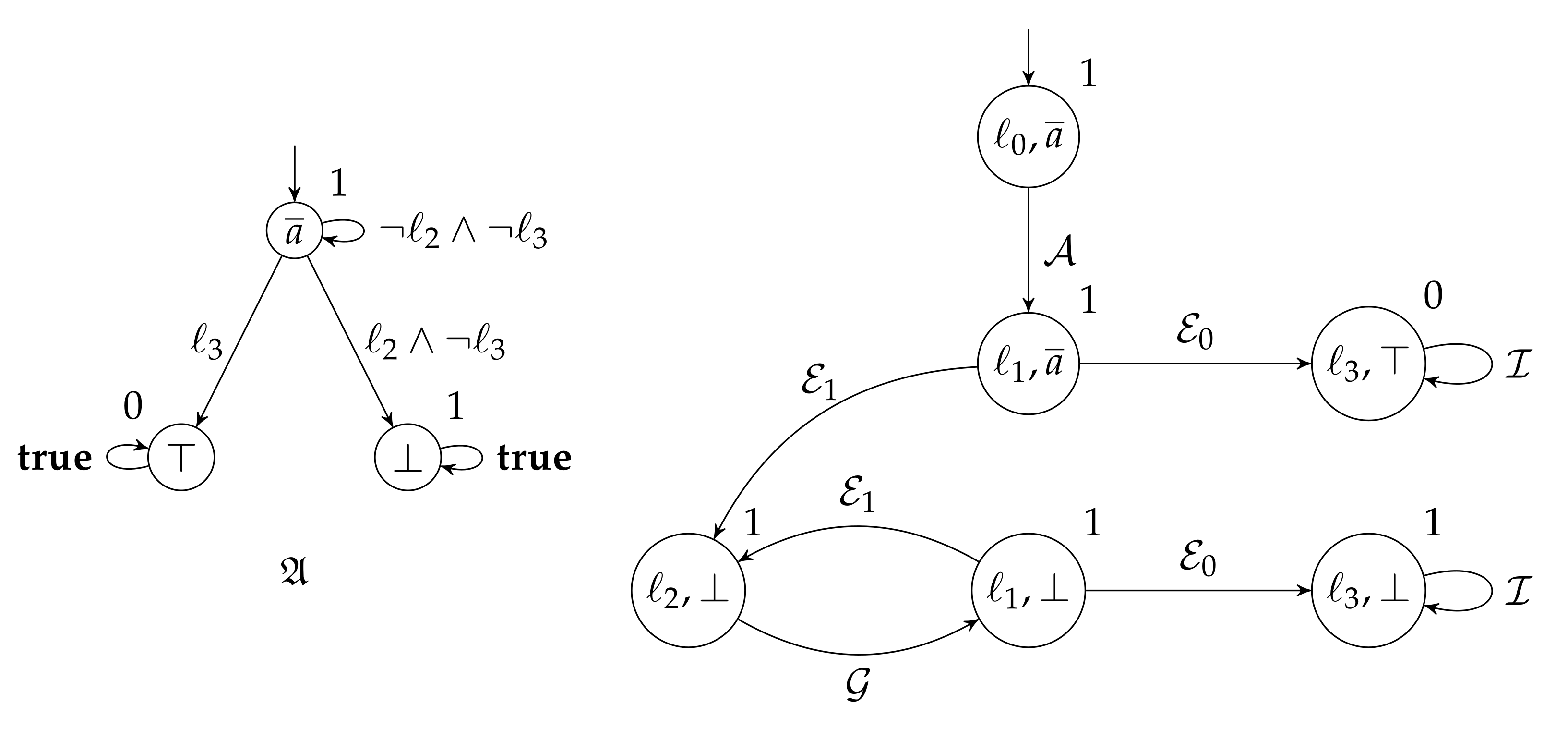
Example 1.
As an example of application of quantum CTL, consider the QMC shown in Figure 1 and its labelled counterpart where each classical state obtains label , that is, we only assign the state name as the label for the state. As formula, consider , which requires to check whether the super-operator corresponding to the paths that eventually reach without passing through is at least . The algorithm for model checking this property works as follows: we start from the state properties in the leaves of the parsing tree of , that is, and , and we compute and . Then, we compute . Now we can compute the super-operator associated with the paths satisfying the path formula .
We initialize the sets , , and as , , and . The Bellman equations for the states in are the following, once we plug in the known values and for the states in and , respectively: and , which correspond to the least fixed point of the function , where
used in [44] (Theorem 5.1). The final result is and , for which we have , as well as . Thus, we obtain , since is the only state from which the computed super-operator is at least .
3.3. Complexity of the QCTL Model Checking Problem
As said at the beginning of this section, textbooks like [26,27] provide a detailed analysis of the model checking algorithms for CTL and PCTL, and they show that such algorithms are efficient. More precisely, such algorithms are polynomial in both the size of the model and the size of the state formula ; the size of is defined [47] as the number of logical connectives and temporal operators in plus the sum of the size of each bounded temporal operators occurring in .
This polynomial complexity carries over the QCTL model checking problem: according to [44], the complexity is polynomial in the size of , of , and the dimension of the Hilbert space .
4. Model Checking Fidelity Properties
The quantum CTL logic we have considered in the previous sections focus on the probability of events, as carried by the computed super-operator. For instance, when model checking an LQMC against a CTL formula , we solve the problem to check whether for some given and (cf. Definition 3). This means, more precisely, to check whether, for each , the trace of is bounded by the trace of .
Quantum CTL is not able to characterize the effect of the super-operators on the quantum states, unless this is reflected on the probability value of their trace. This means, for instance, that the effect of a measurement can be recognized, since the associated probability value is likely to decrease; on the other hand, a bit flip remains undetected, since the whole probability mass is preserved.
To express properties about how well the super-operator modelled by the QMC preserves the quantum state it is applied on a different operator is needed, such as a fidelity operator. The logic we consider is the Fidelity CTL logic (FCTL) proposed in [50], also based on CTL. (The authors of [50] call this logic Quantum CTL. Instead, we call it Fidelity CTL to avoid confusion with the homonym logic in Section 3.) As such, this logic is essentially the same as the classical and probabilistic CTL from literature, and QCTL considered in Section 3. The only difference is on the operator wrapping the path formulas: instead of using the universal ∀, existential ∃, probabilistic , or quantum operators, FCTL uses the fidelity operator , to check whether the fidelity is bounded by . (For uniformity of notation, we use the operator instead of the operator that is used in [50]).
4.1. The Model Checking Problem
Similarly to the other model checking problems, we are given the LQMC and the property we want to verify. The property is usually provided as an FCTL state formula respecting the following grammar:
where , , is a threshold, and . Note that all other comparisons, such as <, >, =, and ≠, that could be used as ∼ in can be derived from ≤ and ≥ with the help of conjunction and negation.
As we can see, the only difference between QCTL and FCTL is that has been replaced with . This means that also the semantics of FCTL differs from the one of QCTL only for this path quantifier. We give the full semantics of FCTL for completeness. Given a state and a path , we have
Given a super-operator , the operator is defined as
where
When is a pure state , then ; moreover, by the joint concavity property (cf. [56] (Exercise 9.19)), it holds that .
The model checking problem for LQMCs against an FCTL state formula is the natural counterpart of the one against QCTL (cf. Definition 3).
Definition 4.
Let be an LQMC, be a state, and φ be an FCTL state formula. The model checking problem for against φ asks to verify whether holds.
4.2. The Standard Bottom–Up Approach
As one can reasonably expect, the model checking algorithm for FCTL is analogous to the one for QCTL: it follows a bottom-up approach to compute the sets for each the state subformula occurring in the formula we need to verify. Everything is the same, except for the evaluation of . For this, first the matrix representation of the super-operator is obtained, which corresponds to the analogous computation for QCTL. Then, the expression is evaluated by converting it to the quantified constraint , where and . The resulting constraint, after some appropriate manipulation, is then verified by means of the existential theory of the reals.
Example 2.
As an example of the application of the fidelity operator, consider the QMC for the loop program depicted in Figure 1 and the fidelity formula . We have already computed in Example 1 the super-operators corresponding to the path formula for each state , that is, , , , and . The formula holds in the state if the corresponding super-operator is such that ; this holds only when (cf. [50]), which is true only for .
4.3. Complexity of the FCTL Model Checking Problem
Since FCTL differs from CTL, PCTL, and QCTL only for one operator, the detailed complexity analysis available in literature (see, e.g., [26,27,58]) for this kind of logic carries over to FCTL [50]. However, the presence of the fidelity operator increases the resulting complexity from polynomial to exponential [50] (Theorem 5.12).
5. Model Checking LTL and -Regular Properties
As we mentioned in the introduction, LTL and -regular properties are well suited for describing the behavior of a system in the long run, such as its liveness (e.g., the system never crashes), repeated reachability (e.g., the system is ready to accept requests again and again), and fairness (e.g., if the system has to make a choice infinitely often, all options are chosen infinitely often) properties. This kind of properties has been studied extensively for classical Markov chains [27,59,60,61]. In the classical setting, the usual approach to compute the probability that a certain LTL property is satisfied in a Markov chain is to adopt an automaton-based approach, as the one introduced by Vardi and Wolper for program verification [62]. This approach works as follows; see, e.g., [26,27] for more details.
5.1. The Model Checking Problem
We start with the model and the property we want to verify. The property is usually given as an LTL formula, that is, a formula expressible according to the following grammar:
where is taken from the given finite set of atomic propositions. In addition, the syntactic sugar shared with CTL, we also consider the Globally/Always temporal operator , sometimes written as .
The semantics of LTL is analogous to the one of CTL, in particular for the temporal operators. We call word an infinite sequence of sets of atomic propositions . We say that w satisfies φ, denoted by , in the following cases:
where . We denote the set of all words satisfying by .
The model checking problem for LQMCs against an LTL formula is formalized as follows.
Definition 5.
Let be an LQMC, be a state, and φ be an LTL formula. Given and , the model checking problem for against φ asks to verify whether holds.
The model checking problem for LQMCs against an -regular property is defined analogously.
Definition 6.
Let be an LQMC, be a state, and be an ω-regular property. Given and , the model checking problem for against asks to verify whether holds.
5.2. The Standard Automata-Based Approach
In the standard automata-based approach [62] to LTL model checking in the context of classical Markov chains, the first step requires to transform the given LTL formula into an equivalent nondeterministic Büchi automaton accepting the same language as , i.e., ; such an automaton always exists (cf. [27] (Theorem 5.37)). Since nondeterministic Büchi automata are as expressive as -regular languages (cf. [27] (Theorem 4.32)), we can also solve the model checking problem against -regular properties, by the same approach.
The nondeterminism present in the Büchi automaton, however, does not play well with the computation of the probability measure. For this motivation, the Büchi automaton needs to be made deterministic; however, deterministic Büchi automata are strictly less expressive than nondeterministic ones (cf. [27] (Theorem 4.50)), so more powerful deterministic automata need to be used. Therefore, the nondeterministic Büchi automaton is transformed into an equivalent deterministic automaton with a more complex acceptance condition, such as Rabin, Streett, Muller, or parity (cf. [63,64,65]). The construction of such deterministic automata usually makes use of a variant of the Safra’s [66] approach, see for instance [67,68], or some of the more recent Safraless constructions, such as the ones proposed in [69,70,71].
Once the deterministic automaton is available, it can be combined with the Markov chain as the product ; this product is in practice a Markov chain extended with the information about the paths that are accepted by the automaton (i.e., the paths that satisfy the formula ); we call such a product a parity Markov chain, when is a parity automaton. As the last step, the probability of the accepting paths is computed. Since all accepting paths need to be infinite, the finite number of states of implies that such paths need to become trapped into a set of states from which they cannot escape, that is, the states that form a bottom strongly connected component (BSCC). Intuitively, a BSCC is composed by states that can be reached by each other, and all their successors are also in the same BSCC. These BSCCs can be computed by means of algorithms operating on the graph structure of the product Markov chain; the outcome of these algorithms is a classification of the states of as those belonging to a BSCC and the transient states, i.e., all other states. Since only states in a BSCC can be visited infinitely often with strictly positive probability, the acceptance condition provided by is used to mark each BSCC as either accepting or rejecting. As the last step, the probability that holds in a given state s of the Markov chain is computed by finding the unique solution of a systems of equations: if s belongs to an accepting BSCC, the probability is 1; if s belongs to a rejecting BSCC, the probability is 0; if s is a transient state, then the probability satisfies the Bellman equation , where is the probability in to make a transition from s to , i.e., the probabilistic counterpart of in quantum Markov chains.
5.3. The Standard Automata-Based Approach Does Not Work Directly for LQMCs
In the remainder of this section, we present how the approach used to check Markov chains against -regular properties can be extended to quantum Markov chains.
The only difference between classical Markov chains and quantum Markov chains is the use of super-operators instead of probability values to decorate the transitions; this difference, however, has a considerable effect on the model checking algorithm, as pointed out in, e.g., [49,72]. Consider the two Markov chains, enriched with a parity acceptance condition, shown in Figure 2. The parity acceptance is provided by the priorities 0 and 1 labelling the classical states , , and . As we will see more formally below, a path is accepted if the minimum priority occurring infinitely often is even. This means, for instance, that the path is accepted, since its corresponding sequence of priorities is whose minimum priority occurring infinitely often is 0; on the other hand, the path is rejecting, since its minimum priority occurring infinitely is 1.
The Markov chain on the left of Figure 2 is a classical one where transitions are governed by the two transition probabilities p and with . The Markov chain on the right is a quantum one governed by the two super-operators and , such that and . It is obvious that both Markov chains have the same classical state space, thus they have exactly the same underlying graph. If we would define the BSCCs just by looking at the underlying graph, they would have the same set of BSCCs, namely just the single BSCC , and the same single transient state . However, we will see that this BSCC technique does not help in the evaluation of parity QMCs.
In the classical Markov chains model, is a transient state that will eventually reach almost surely the unique BSCC . Thus, its priority makes no difference. Since the probability that both states in the BSCC are visited infinitely often is 1, we have that the BSCC is marked as accepting, since the minimum priority of its states is 0. Since the BSCC is accepting and all paths from eventually enter almost surely, we find that the overall probability of the paths eventually becoming trapped in an accepting BSCC is 1 for all states.
Consider now the quantum Markov chain on the right part of Figure 2 and assume that and . Note that for it holds and . It is easy to check that if we start from , the infinite path , with the corresponding nonzero super-operator , never leaves to reach the other states and . This means that cannot be considered a BSCC, since cannot reach itself almost surely, i.e., with super-operator . At the same time, cannot be considered a transient state, since it will not eventually reach a BSCC almost surely. Therefore, the first problem we encounter is that a state in a QMC cannot be classified either as transient or as belonging to a BSCC, as happens for classical Markov chains. In addition to this problem with the classification of , we also have a second problem, namely, that the infinite path has minimum priority 0, so it must be taken into account when computing the super-operator corresponding to the accepting paths. This means that it does not suffice to look only at the states as performed for classical parity Markov chains, but we need to consider all possible paths.
Consider now the state : we have only two infinite paths occurring with nonzero super-operator, namely with associated super-operator and priority 0, and with associated super-operator and priority 0. Thus, the super-operator corresponding to the accepting paths in state is . The situation for is however different: we still have only two paths, namely with associated super-operator and priority 0, and having super-operator and priority 1. Thus, the value in is , that is different from in . Therefore, we have a third problem, namely, we cannot associate the same value to all states in a BSCC, as we can do for classical Markov chains, but each state must be evaluated individually.
Let us reason more about what happens along the path : its corresponding super-operator is , as effect of the composition of the two orthogonal super-operators and in the first two transitions and , respectively. In practice, it is as the first transition from to , decorated with , “disables” the second transition from to , decorated with . In other words, it is like we are missing the Markovian property that allows us to forget about the past, namely that the transitions we can perform depend only on the current state, not on how we reached it. Therefore, we cannot assume that the underlying graph is immutable, since the previous transitions we performed to reach the current state might change the available edges in the underlying graph. This means that we cannot just use the standard BSCC decomposition algorithms on the underlying graph to solve the LTL and -regular model checking problem for LQMCs: neither are BSCCs reached with certainty, nor do all states of a BSCC have the same value. In addition, the value of a state in a BSCC can be different from both and .
In order to overcome these problems, in [49] we proposed an alternative approach: instead of relying on the graph structure of the product , we transformed it into a single super-operator and we considered the BSCC decomposition of the classical-quantum Hilbert space induced by this super-operator, i.e., the tensor product of the classical state space with the quantum one. By operating on this larger Hilbert space, we have the information we need to solve the model checking problem for -regular properties for labelled quantum Markov chains.
5.4. Parity Automata and Parity Quantum Markov Chains
We shortly recall a well-known mechanism to decide whether a word is included in a given -regular language. Recall that is called -regular if it is the language of some nondeterministic Büchi automaton (cf. [27] (Theorem 4.32)) and that nondeterministic Büchi automata are equivalent to parity automata (cf. [63,64,65]). A parity automaton is defined formally as follows.
Definition 7.
A (deterministic) parity automaton (PA) is a tuple , where
- A is a finite set of automaton states;
- is the initial state;
- is a finite set of atomic propositions;
- is a transition function; and
- is a priority function.
A path of is an infinite sequence , such that and for all , . We extend the priority function to paths by setting . We use to denote the set of all paths of . The language of is defined as
As we have enriched QMCs with labels, obtaining LQMCs (cf. Definition 2), we also decorate QMCs with parity conditions, so to obtain parity QMCs; these will be useful to represent the result of the product of an LQMC and a PA, that we will present later.
Definition 8.
A parity quantum Markov chain (PQMC) is a tuple , where is a QMC and is a priority function.
As we have done for LQMCs, we extend in the natural way the notion of paths, measures, etc. to PQMCs and we set . We define the value of a PQMC in as
Parity QMCs can be obtained by combining together an LQMC and a PA; in practice, the PA just follows the evolution of the LQMC by synchronizing on the labels of the classical states that are visited by the LQMC.
Definition 9.
The product of an LQMC and a PA with the same set of atomic propositions is the PQMC where
- ;
- if , and otherwise; and
- .
An important property that is used in the model checking problem of an LQMC against an -regular property recognized by is that the value of is trace equivalent to the super-operator corresponding to in . Formally, by [49] (Lemma 9) we have that for any ,
This property is the expected quantum counterpart of the product Markov chain used for solving the model checking problem of classical Markov chains against LTL and -regular properties (cf. [27]). This equivalence ensures that the super-operator we obtain in the product PQMC is equivalent to the one corresponding to the paths of the LQMC satisfying the given -regular property, and this is needed to justify the correctness of the automata-based approach to model checking.
Example 3.
As an example of the parity construction, consider again the QMC shown in Figure 1 and the LTL formula .
On the left part of Figure 3 we present the parity automaton corresponding to the formula . The automaton has 3 states, namely , ⊥, and ⊤; the value assigned by the priority function to each state is given as the number near the state: this means that all states have priority 1 except for . The transition relation is given by the depicted arrows, where we encode the sets of atomic propositions by a Boolean formula: for instance, the formula is satisfied by all subsets A of , such that ; similarly, the formula is satisfied by all subsets A of , such that but .
5.5. Computing PQMC Values
As we have seen in Section 5.3, it is not enough to compute the BSCCs by looking only at the classical states of the product PQMC. The solution adopted by [49] is to encode the behavior of into a single super-operator acting on the extended Hilbert space representing both the classical states and the super-operators decorating the transitions. This is obtained by taking the tensor product of the classical state space and the quantum one; then the notion of BSCC subspaces for super-operators, as defined in [73], is used in the computation of the PQMC values. The intuition underlying this extended construction is to keep track of the classical states reached step by step in the part of , and to accumulate the effects of the super-operators decorating the taken transitions on the part of . This allows us to overcome the problem of the BSCC decomposition of the underlying graph of the given PQMC: as we have seen in Section 5.3, by performing a transition we might change the underlying graph, since some transition might be disabled as effect of the composition of super-operators; this does not happen in the classical and probabilistic setting, where the underlying graph is immutable.
Let be a super-operator acting on ; given a subspace X of , we call X:
- invariant for if ;
- a BSCC of if holds for each pure state , where is the reachable subspace of starting in ;
- transient if for each , where is the projection onto X.
Intuitively, we have that the probability of remaining forever in a transient subspace X tends to 0, as happens for the transient states in a classical Markov chain. Similarly, it is not possible to leave a BSCC X, and eventually all elements of X are visited again and again, as happens for states in the BSCCs of a classical Markov chain.
We are now ready to present how to combine together the classical part and the quantum part of a PQMC. Let be a PQMC on ; for each , let be the set of Kraus operators with as set of indexes for the super-operator . Following [72], let be the super-operator acting on the extended Hilbert space , where is the -dimensional Hilbert space with orthonormal basis .
For each , let and . To see how encodes the behavior of , consider the following steps, which exactly capture the intended meaning of .
- 1.
- A projective measurement is performed on the classical system to determine the current classical state.
- 2.
- If the measurement outcome of M is s, then the quantum measurement is performed on the quantum system .
- 3.
- If the observed outcome of is , then the classical state is set to be .
The super-operator enjoys a couple of nice properties: starting from a product initial state, the classical and quantum systems remain separable (disentangled) along the whole execution (cf. [49] (Lemma 11)); moreover, each fixed point state of , i.e., , has the form . According to [73], we find that any BSCC of can be spanned by pure states of the form where and .
We are now ready to collect all BSCCs of and classify them according to their acceptance condition. Given a BSCC B of , let
be the set of classical states supported in B. Note that it is possible to have for two different BSCCs B and ; this happens when there are two states and with . However, this is not a real problem: as shown by [49] (Lemma 12), two BSCCs are orthogonal as long as they differ on at least one classical state.
Given the set of all BSCCs of , we can organize it with respect to the minimal priority assigned to the classical states in each BSCC. For a priority , let be the span of all BSCCs of whose minimal priority is k, that is,
Similarly, let and be the spans of all BSCCs with the minimal priority being less than and larger than k, respectively. Since , , and have different sets of classical states, they are pairwise orthogonal by [49] (Lemma 12). This implies, by [73], that can be decomposed uniquely into
where T is the maximum transient subspace of .
An important result (cf. [49] (Lemma 13)) is that the BSCCs in , , and do not interfere with each other: let denote the probability that k is the lowest priority occurring infinitely often from the initial state . Then, we have that:
- if , then ;
- if , then ; and
- if , then ,
that is, once we enter with probability , we will see k as the minimum priority almost surely; instead, if we enter or , we will see k as minimum priority with probability 0. In practice, acts like the standard BSCC with minimum priority k in classical Markov chains.
It now remains to collect all with even priority k to obtain the accepting BSCCs, and combine together their super-operators. This is formalized as follows.
Theorem 1
([49] (Corollary 15)). Let be a PQMC. Then, for any ,
where is the partial trace super-operator, such that , where is the projection super-operator onto , , and .
Similarly to the QCTL case (cf. Section 3), the value is not computed exactly, but only a trace equivalent super-operator is obtained. This is in line with the statement of [44] (Theorem 3.2), saying that the super-operator valued measure for a QMC (hence, for a PQMC) is well-defined only up to the trace equivalence ≂, already at the level of the measure for the measurable space . This means that we are not able to compute the exact super-operator corresponding to a measurable set of paths, but only a super-operator in the same ≂-equivalence class. This suffices for our purposes, since LTL and -regular model checking for LQMCs (as well as the QCTL model checking) only look for the probability of satisfying the given property, which is preserved by ≂.
As an application of the above construction, consider the right part of Figure 3, where we show the product of the QMC shown in Figure 1 and the PA encoding the formula . It is easy to observe that, for this specific case, we have only one accepting BSCC, composed only by the state , and that the super-operator corresponding to the paths leading to it is , the same as we computed in Example 1, as expected.
As another application of the above construction, consider again the PQMC depicted on the right of Figure 2 where the super-operators decorating the transitions are and . Then, the super-operator encoding is
In practice, for each pair of states s and t for which , we add , which can be intuitively interpreted as: we transition from s to t while performing . We can now decompose into the BSCCs and the maximal transient space, obtaining that the maximal transient space of is and that the BSCCs are
Since the priorities range over , we obtain only with even minimum priority, with corresponding projection super-operator (in Kraus notation)
which is also the projection super-operator occurring in Theorem 1.
Regarding the super-operator , we first compute its components. For any , we have and , where
Thus, and
Lastly, we have and . By Theorem 1, it follows that
These values coincide with the informal discussion we have given in Section 5.3.
5.6. Complexity of the LTL and -Regular Model Checking Problem
A detailed algorithm providing the necessary computational steps implementing the construction given above can be found in [49]. Its complexity for computing the matrix representation of is polynomial in the size of the given PQMC and in the dimension of its Hilbert space.
If we want to express the size of the product PQMC in terms of the original LQMC and of the LTL formula , then is linear in the size of and double exponential in the size of . The double exponential blowup is common in model checking LTL properties: the first exponential blowup occurs in the translation from to an equivalent nondeterministic Büchi automaton; the second blowup is caused by its determinization as a Rabin, a Streett, a Muller, or a parity automaton. These blowups cannot be avoided (cf. [26,27,63]).
6. Conclusions
In this paper we have presented three logics and relative model checking algorithms for quantum Markov chains given in literature: quantum CTL, quantum LTL and -regular properties, and fidelity CTL. The former two kinds of properties focus on evaluating the probability of certain events; the latter, instead, looks for how well the super-operator modelled by the LQMC preserves the quantum states it is applied on.
The algorithms for the quantum counterparts of CTL and LTL follow the steps of the algorithms already developed for these logics in the setting of classical and probabilistic model checking. The quantum nature of the system to be checked, however, prevents the naïve adaptation of these algorithms, in particular for LTL and -regular properties: the usual BSCC decomposition of the underlying graph fails, so a similar decomposition needs to be performed in an extended Hilbert space representing both the classical and the quantum states of the product PQMC. The algorithm for the computation of the states satisfying the fidelity operator, instead, is newly designed, since fidelity is a concept strictly related to quantum systems that has no counterparts in classical and probabilistic systems.
Funding
This work was supported in part by the Guangdong Science and Technology Department (Grant No. 2018B010107004) and by the National Natural Science Foundation of China (Grants Nos. 61836005, 62102407, 62172019).
Institutional Review Board Statement
Not applicable.
Informed Consent Statement
Not applicable.
Data Availability Statement
Not applicable.
Conflicts of Interest
The author declares no conflict of interest.
References
- Dijkstra, E.W. The Humble Programmer. Commun. ACM 1972, 15, 859–866. [Google Scholar] [CrossRef] [Green Version]
- Clarke, E.M.; Emerson, E.A. Design and Synthesis of Synchronization Skeletons Using Branching-Time Temporal Logic. In Logic of Programs; Lecture Notes in Computer Science; Springer: Berlin/Heidelberg, Germany, 1981; Volume 131, pp. 52–71. [Google Scholar]
- Queille, J.; Sifakis, J. Specification and verification of concurrent systems in CESAR. In Symposium on Programming; Lecture Notes in Computer Science; Springer: Berlin/Heidelberg, Germany, 1982; Volume 137, pp. 337–351. [Google Scholar]
- Burch, J.R.; Clarke, E.M.; McMillan, K.L.; Dill, D.L. Sequential Circuit Verification Using Symbolic Model Checking. In Proceedings of the 27th ACM/IEEE Design Automation Conference, Orlando, FL, USA, 24–28 June 1990; pp. 46–51. [Google Scholar]
- Clarke, E.M.; Filkorn, T.; Jha, S. Exploiting Symmetry In Temporal Logic Model Checking. In CAV; Lecture Notes in Computer Science; Springer: Berlin/Heidelberg, Germany, 1993; Volume 697, pp. 450–462. [Google Scholar]
- Gupta, A. Formal Hardware Verification Methods: A Survey. Formal Methods Syst. Des. 1992, 1, 151–238. [Google Scholar] [CrossRef]
- Kropf, T. Introduction to Formal Hardware Verification; Springer: Berlin/Heidelberg, Germany, 1999. [Google Scholar]
- Yoeli, M. Formal Verification of Hardware Design; IEEE Computer Society Press: Piscataway, NJ, USA, 1990. [Google Scholar]
- Liggesmeyer, P.; Rothfelder, M.; Rettelbach, M.; Ackermann, T. Qualitätssicherung Software-basierter technischer Systeme—Problembereiche und Lösungsansätze. Inform. Spektrum 1998, 21, 249–258. [Google Scholar] [CrossRef]
- Peled, D.A. Software Reliability Methods; Texts in Computer Science; Springer: Berlin/Heidelberg, Germany, 2001. [Google Scholar]
- Rushby, J.M.; von Henke, F.W. Formal Verification of Algorithms for Critical Systems. IEEE Trans. Softw. Eng. 1993, 19, 13–23. [Google Scholar] [CrossRef]
- Tretmans, J.; Wijbrans, K.; Chaudron, M.R.V. Software Engineering with Formal Methods: The Development of a Storm Surge Barrier Control System Revisiting Seven Myths of Formal Methods. Formal Methods Syst. Des. 2001, 19, 195–215. [Google Scholar] [CrossRef]
- Wijbrans, K.; Buve, F.; Rijkers, R.; Geurts, W. Software Engineering with Formal Methods: Experiences with the Development of a Storm Surge Barrier Control System. In FM; Lecture Notes in Computer Science; Springer: Berlin/Heidelberg, Germany, 2008; Volume 5014, pp. 419–424. [Google Scholar]
- Holzmann, G.J. Design and Validation of Computer Protocols; Prentice-Hall, Inc.: Hoboken, NJ, USA, 1990. [Google Scholar]
- Holzmann, G.J. Design and Validation of Protocols: A Tutorial. Comput. Netw. ISDN Syst. 1993, 25, 981–1017. [Google Scholar] [CrossRef]
- Holzmann, G.J. The Theory and Practice of A Formal Method: NewCoRe. In IFIP Congress (1); IFIP Transactions; North-Holland: Amsterdam, The Netherlands, 1994; Volume A-51, pp. 35–44. [Google Scholar]
- Clarke, E.M.; Grumberg, O.; Hiraishi, H.; Jha, S.; Long, D.E.; McMillan, K.L.; Ness, L.A. Verification of the Futurebus+ Cache Coherence Protocol. Formal Methods Syst. Des. 1995, 6, 217–232. [Google Scholar] [CrossRef]
- Lowe, G. Breaking and Fixing the Needham-Schroeder Public-Key Protocol Using FDR. Softw. Concepts Tools 1996, 17, 93–102. [Google Scholar]
- Chen, T.; Diciolla, M.; Kwiatkowska, M.Z.; Mereacre, A. Quantitative verification of implantable cardiac pacemakers over hybrid heart models. Inf. Comput. 2014, 236, 87–101. [Google Scholar] [CrossRef]
- Chan, W.; Anderson, R.J.; Beame, P.; Burns, S.; Modugno, F.; Notkin, D.; Reese, J.D. Model Checking Large Software Specifications. IEEE Trans. Softw. Eng. 1998, 24, 498–520. [Google Scholar] [CrossRef]
- Staunstrup, J.; Andersen, H.R.; Hulgaard, H.; Lind-Nielsen, J.; Larsen, K.G.; Behrmann, G.; Kristoffersen, K.J.; Skou, A.; Leerberg, H.; Theilgaard, N.B. Practical Verification of Embedded Software. Computer 2000, 33, 68–75. [Google Scholar] [CrossRef]
- Havelund, K.; Lowry, M.R.; Penix, J. Formal Analysis of a Space-Craft Controller Using SPIN. IEEE Trans. Softw. Eng. 2001, 27, 749–765. [Google Scholar] [CrossRef] [Green Version]
- Holzmann, G.J.; Najm, E.; Serhrouchni, A. SPIN Model Checking: An Introduction. Int. J. Softw. Tools Technol. Transf. 2000, 2, 321–327. [Google Scholar] [CrossRef]
- Bozzano, M.; Cimatti, A.; Katoen, J.; Katsaros, P.; Mokos, K.; Nguyen, V.Y.; Noll, T.; Postma, B.; Roveri, M. Spacecraft early design validation using formal methods. Reliab. Eng. Syst. Saf. 2014, 132, 20–35. [Google Scholar] [CrossRef] [Green Version]
- Hoque, K.A.; Mohamed, O.A.; Savaria, Y. Towards an accurate reliability, availability and maintainability analysis approach for satellite systems based on probabilistic model checking. In Proceedings of the 2015 Design, Automation & Test in Europe Conference & Exhibition (DATE), Grenoble, France, 9–13 March 2015; pp. 1635–1640. [Google Scholar]
- Clarke, E.M.; Henzinger, T.A.; Veith, H.; Bloem, R. (Eds.) Handbook of Model Checking; Springer: Berlin/Heidelberg, Germany, 2018. [Google Scholar]
- Baier, C.; Katoen, J. Principles of Model Checking; MIT Press: Cambridge, MA, USA, 2008. [Google Scholar]
- Bérard, B.; Bidoit, M.; Finkel, A.; Laroussinie, F.; Petit, A.; Petrucci, L.; Schnoebelen, P.; McKenzie, P. Systems and Software Verification, Model-Checking Techniques and Tools; Springer: Berlin/Heidelberg, Germany, 2001. [Google Scholar]
- Clarke, E.M.; Grumberg, O.; Peled, D.A. Model Checking; MIT Press: Cambridge, MA, USA, 2001. [Google Scholar]
- Huth, M.; Ryan, M.D. Logic in Computer Science—Modelling and Reasoning about Systems; Cambridge University Press: Cambridge, UK, 2000. [Google Scholar]
- Schneider, K. Verification of Reactive Systems—Formal Methods and Algorithms; Texts in Theoretical Computer Science; An EATCS Series; Springer: Berlin/Heidelberg, Germany, 2004. [Google Scholar]
- Ben-Ari, M. Principles of the SPIN Model Checker; Springer: Berlin/Heidelberg, Germany, 2008. [Google Scholar]
- McMillan, K.L. Symbolic Model Checking; Kluwer: Alphen aan den Rijn, The Netherlands, 1993. [Google Scholar]
- Bennett, C.H.; Brassard, G. Quantum cryptography: Public-key distribution and coin tossing. In Proceedings of the IEEE International Conference on Computer, Systems and Signal Processing, Bangalore, India, 9–12 December 1984; pp. 175–179. [Google Scholar]
- Bennett, C.H.; Brassard, G. Quantum cryptography: Public key distribution and coin tossing. Theor. Comput. Sci. 2014, 560, 7–11. [Google Scholar] [CrossRef]
- Bennett, C.H. Quantum cryptography using any two nonorthogonal states. Phys. Rev. Lett. 1992, 68, 3121. [Google Scholar] [CrossRef]
- Bennett, C.H.; Wiesner, S.J. Communication Via One- and Two-particle Operators on Einstein-Podolsky-Rosen States. Phys. Rev. Lett. 1992, 69, 2881–2884. [Google Scholar] [CrossRef] [PubMed] [Green Version]
- Shor, P.W. Algorithms for Quantum Computation: Discrete Logarithms and Factoring. In Proceedings of the 35th Annual Symposium on Foundations of Computer Science, Santa Fe, NM, USA, 20–22 November 1994; pp. 124–134. [Google Scholar]
- Gay, S.J.; Nagarajan, R.; Papanikolaou, N. Probabilistic model-checking of quantum protocols. In Proceedings of the 2nd International Workshop on Developments in Computational Models, Venice, Italy, 16 July 2006. [Google Scholar]
- Papanikolaou, N. Model Checking Quantum Protocols. Ph.D. Thesis, University of Warwick, Coventry, UK, 2009. [Google Scholar]
- Gay, S.J.; Nagarajan, R.; Papanikolaou, N. QMC: A Model Checker for Quantum Systems. In CAV; Lecture Notes in Computer Science; Springer: Berlin/Heidelberg, Germany, 2008; Volume 5123, pp. 543–547. [Google Scholar]
- Hung, W.N.N.; Song, X.; Yang, G.; Yang, J.; Perkowski, M.A. Quantum logic synthesis by symbolic reachability analysis. In Proceedings of the 41st Annual Design Automation Conference, San Diego, CA, USA, 7–11 June 2004; pp. 838–841. [Google Scholar]
- Hung, W.N.N.; Song, X.; Yang, G.; Yang, J.; Perkowski, M.A. Optimal synthesis of multiple output Boolean functions using a set of quantum gates by symbolic reachability analysis. IEEE Trans. Comput. Aided Des. Integr. Circuits Syst. 2006, 25, 1652–1663. [Google Scholar] [CrossRef] [Green Version]
- Feng, Y.; Yu, N.; Ying, M. Model checking quantum Markov chains. J. Comput. Syst. Sci. 2013, 79, 1181–1198. [Google Scholar] [CrossRef]
- Pnueli, A. The Temporal Logic of Programs. In Proceedings of the 18th Annual Symposium on Foundations of Computer Science, Providence, RI, USA, 31 October–2 November 1977; pp. 46–57. [Google Scholar]
- Emerson, E.A.; Halpern, J.Y. “Sometimes” and “Not Never” revisited: On branching versus linear time temporal logic. J. ACM 1986, 33, 151–178. [Google Scholar] [CrossRef]
- Hansson, H.; Jonsson, B. A Logic for Reasoning about Time and Reliability. Formal Aspects Comput. 1994, 6, 512–535. [Google Scholar] [CrossRef] [Green Version]
- Bianco, A.; de Alfaro, L. Model Checking of Probabalistic and Nondeterministic Systems. In FSTTCS; Lecture Notes in Computer Science; Springer: Berlin/Heidelberg, Germany, 1995; Volume 1026, pp. 499–513. [Google Scholar]
- Feng, Y.; Hahn, E.M.; Turrini, A.; Ying, S. Model Checking Omega-regular Properties for Quantum Markov Chains. In CONCUR; Schloss Dagstuhl—Leibniz-Zentrum für Informatik: Wadern, Germany, 2017; Volume 85, pp. 35:1–35:16. [Google Scholar]
- Xu, M.; Fu, J.; Mei, J.; Deng, Y. An Algebraic Method to Fidelity-based Model Checking over Quantum Markov Chains. arXiv 2021, arXiv:2101.04971. [Google Scholar]
- Duan, Z.; Niu, L. Some properties of quantum fidelity in infinite-dimensional quantum systems. Int. J. Quantum Inf. 2018, 16, 1850028. [Google Scholar] [CrossRef]
- Uhlmann, A. On “Partial” Fidelities. Rep. Math. Phys. 2000, 45, 407–418. [Google Scholar] [CrossRef] [Green Version]
- Burrell, A.H.; Szwer, D.J.; Webster, S.C.; Lucas, D.M. Scalable simultaneous multiqubit readout with 99.99% single-shot fidelity. Phys. Rev. A 2010, 81, 040302. [Google Scholar] [CrossRef] [Green Version]
- Myerson, A.H.; Szwer, D.J.; Webster, S.C.; Allcock, D.T.C.; Curtis, M.J.; Imreh, G.; Sherman, J.A.; Stacey, D.N.; Steane, A.M.; Lucas, D.M. High-Fidelity Readout of Trapped-Ion Qubits. Phys. Rev. Lett. 2008, 100, 200502. [Google Scholar] [CrossRef] [Green Version]
- Ying, M.; Feng, Y. Model Checking Quantum Systems: Principles and Algorithms; Cambridge University Press: Cambridge, UK, 2021. [Google Scholar]
- Nielsen, M.A.; Chuang, I.L. Quantum Computation and Quantum Information; Cambridge University Press: Cambridge, UK, 2000. [Google Scholar]
- Selinger, P. A Brief Survey of Quantum Programming Languages. In FLOPS; Lecture Notes in Computer Science; Springer: Berlin/Heidelberg, Germany, 2004; Volume 2998, pp. 1–6. [Google Scholar]
- Feng, Y.; Hahn, E.M.; Turrini, A.; Zhang, L. QPMC: A Model Checker for Quantum Programs and Protocols. In FM; Lecture Notes in Computer Science; Springer: Berlin/Heidelberg, Germany, 2015; Volume 9109, pp. 265–272. [Google Scholar]
- de Alfaro, L. Formal Verification of Probabilistic Systems. Ph.D. Thesis, Stanford University, Stanford, CA, USA, 1997. [Google Scholar]
- Courcoubetis, C.; Yannakakis, M. The Complexity of Probabilistic Verification. J. ACM 1995, 42, 857–907. [Google Scholar] [CrossRef]
- Bustan, D.; Rubin, S.; Vardi, M.Y. Verifying omega-Regular Properties of Markov Chains. In CAV; Lecture Notes in Computer Science; Springer: Berlin/Heidelberg, Germany, 2004; Volume 3114, pp. 189–201. [Google Scholar]
- Vardi, M.Y.; Wolper, P. An Automata-Theoretic Approach to Automatic Program Verification (Preliminary Report). In Proceedings of the First Symposium on Logic in Computer Science, Cambridge, MA, USA, 16–18 June 1986; pp. 332–344. [Google Scholar]
- Grädel, E.; Thomas, W.; Wilke, T. (Eds.) Automata, Logics, and Infinite Games: A Guide to Current Research; Lecture Notes in Computer Science; Springer: Berlin/Heidelberg, Germany, 2002; Volume 2500. [Google Scholar]
- Mostowski, A.W. Regular expressions for infinite trees and a standard form of automata. In Symposium on Computation Theory; Lecture Notes in Computer Science; Springer: Berlin/Heidelberg, Germany, 1984; Volume 208, pp. 157–168. [Google Scholar]
- Emerson, E.A.; Jutla, C.S. Tree Automata, Mu-Calculus and Determinacy (Extended Abstract). In Proceedings of the 32nd Annual Symposium of Foundations of Computer Science, San Juan, PR, USA, 1–4 October 1991; pp. 368–377. [Google Scholar]
- Safra, S. On the Complexity of omega-Automata. In Proceedings of the 29th Annual Symposium on Foundations of Computer Science, White Plains, NY, USA, 24–26 October 1988; pp. 319–327. [Google Scholar]
- Piterman, N. From Nondeterministic Büchi and Streett Automata to Deterministic Parity Automata. Log. Methods Comput. Sci. 2007, 3, 1–21. [Google Scholar] [CrossRef] [Green Version]
- Schewe, S. Tighter Bounds for the Determinisation of Büchi Automata. In FoSSaCS; Lecture Notes in Computer Science; Springer: Berlin/Heidelberg, Germany, 2009; Volume 5504, pp. 167–181. [Google Scholar]
- Kähler, D.; Wilke, T. Complementation, Disambiguation, and Determinization of Büchi Automata Unified. In ICALP (1); Lecture Notes in Computer Science; Springer: Berlin/Heidelberg, Germany, 2008; Volume 5125, pp. 724–735. [Google Scholar]
- Fogarty, S.; Kupferman, O.; Vardi, M.Y.; Wilke, T. Profile trees for Büchi word automata, with application to determinization. Inf. Comput. 2015, 245, 136–151. [Google Scholar] [CrossRef]
- Löding, C.; Pirogov, A. Determinization of Büchi Automata: Unifying the Approaches of Safra and Muller-Schupp. In ICALP; LIPIcs; Schloss Dagstuhl—Leibniz-Zentrum für Informatik: Wadern, Germany, 2019; Volume 132, pp. 120:1–120:13. [Google Scholar]
- Li, L.; Feng, Y. Quantum Markov chains: Description of hybrid systems, decidability of equivalence, and model checking linear-time properties. Inf. Comput. 2015, 244, 229–244. [Google Scholar] [CrossRef]
- Ying, S.; Feng, Y.; Yu, N.; Ying, M. Reachability Probabilities of Quantum Markov Chains. In CONCUR; Lecture Notes in Computer Science; Springer: Berlin/Heidelberg, Germany, 2013; Volume 8052, pp. 334–348. [Google Scholar]
Figure 1.
A simple loop program and its model as a quantum Markov chain.
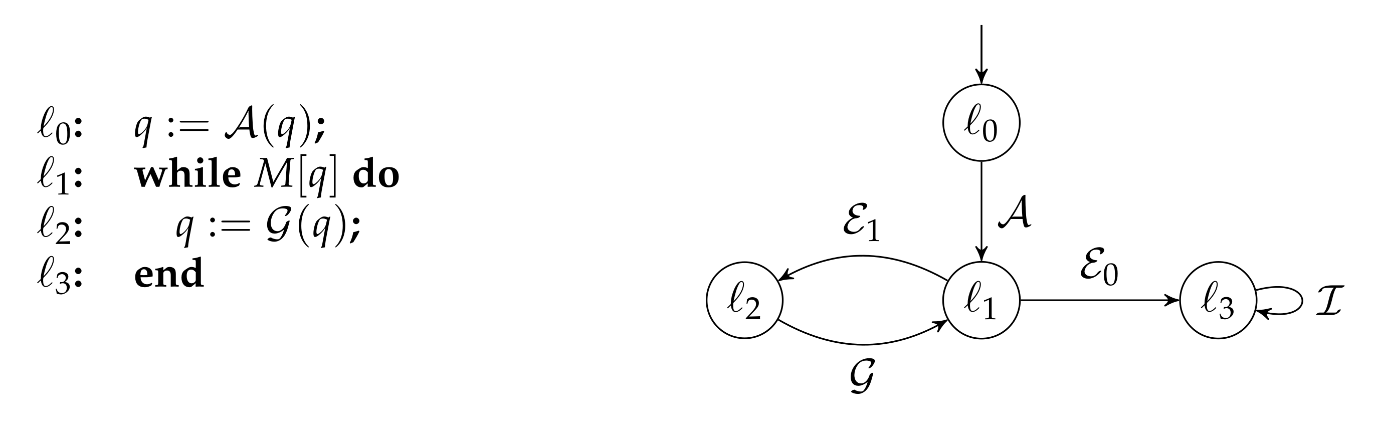
Figure 2.
Example showing that BSCC decomposition for the underlying graph does not work for model checking parity QMCs.
Figure 2.
Example showing that BSCC decomposition for the underlying graph does not work for model checking parity QMCs.

Figure 3.
Parity construction for the QMC from Figure 1 and the LTL formula .
Figure 3.
Parity construction for the QMC from Figure 1 and the LTL formula .
Publisher’s Note: MDPI stays neutral with regard to jurisdictional claims in published maps and institutional affiliations. |
© 2022 by the author. Licensee MDPI, Basel, Switzerland. This article is an open access article distributed under the terms and conditions of the Creative Commons Attribution (CC BY) license (https://creativecommons.org/licenses/by/4.0/).
Share and Cite
MDPI and ACS Style
Turrini, A. An Introduction to Quantum Model Checking. Appl. Sci. 2022, 12, 2016. https://doi.org/10.3390/app12042016
AMA Style
Turrini A. An Introduction to Quantum Model Checking. Applied Sciences. 2022; 12(4):2016. https://doi.org/10.3390/app12042016
Chicago/Turabian StyleTurrini, Andrea. 2022. "An Introduction to Quantum Model Checking" Applied Sciences 12, no. 4: 2016. https://doi.org/10.3390/app12042016
Note that from the first issue of 2016, this journal uses article numbers instead of page numbers. See further details here.