Article

A Novel Dictionary-Based Method to Compress Log Files with Different Message Frequency Distributions

1
Department of Information Systems, ELTE Eötvös Loránd University, 1117 Budapest, Hungary
2
Department of Informatics, J. Selye University, 945 01 Komárno, Slovakia
*
Author to whom correspondence should be addressed.
Appl. Sci. 2022, 12(4), 2044; https://doi.org/10.3390/app12042044
Submission received: 20 December 2021 / Revised: 7 February 2022 / Accepted: 11 February 2022 / Published: 16 February 2022

Abstract

:
In the present day, virtually every application software generates large amounts of log entries during its work. The log files that are made from these entries are a collection of information about what happened while the program was running. This report can be used for multiple purposes such as performance monitoring, maintaining security, or improving business decision making. Log entries are usually generated in a disorganized manner. Using template miners, the different ‘event types’ can be distinguished (each log entry is an event), and the set of all entries is split into disjointed subsets according to the event types. These events consist of two parts. The first is the constant part, which is the same for all occurrences of the same event type. The second is the parameter part, which can be different for each occurrence. Since software mass-produces log files, in our previous paper, we introduced an algorithm that uses the templates mined from the data to create a dictionary, which is then used to encode the log entries, so only the ID and the parameter list would be stored. In this paper, we enhance our algorithm with the use of the frequency of the templates, by encoding the parameters and also making use of Huffman coding. With the use of these measures, compared to the previous 67.4% compression rate, a 94.98% compression rate can be achieved (where compression rate is 1 minus the ratio of the size of the compressed file to the uncompressed size). The running times of the different measures that we used to enhance our algorithm are also compared. We also analyze the difference between the compression rate of the enhanced algorithm and general compressors such as LZMA, Bzip2, and PPMd. We examine whether the size of the log files can be further decreased with the combined use of our enhanced method and the general compressors. We also generate log files that follow different distributions to examine the compression capability if the distribution does not follow the power law. Based on our experiments, we would recommend the use of the MoLFI (Multi-objective Log message Format Identification) template miner method with our enhanced algorithm together with PPMd.

1. Introduction

System logs have many applications due to the fact that they contain important runtime information of software systems. This data is created by logging statements inserted into the source code by programmers. The accumulated runtime data can be used for various purposes, such as anomaly detection, business model mining, or performance monitoring. The authors of [1] propose a new, dynamic methodology of anomaly detection on log files. Instead of treating the log files as static files, they incrementally group log lines within time windows. After that, different cluster analysis techniques are used to find merges or splits between the windows. Then, a self-learning algorithm is used to detect anomalies based on the evolution of the clusters. In [2], a method is proposed that uses both data page tagging and log files to build business models. They use new trends in web development languages to analyze customer behavior. They mainly focus on the diversity of the traces left by Rich Internet Applications (web applications using desktop application characteristics). The authors of [3] introduce a new tool, namely DISTALYZER, that uses machine learning techniques. It deduces associations between different components and their performance with the use of previously extracted system behaviors.
With the large-scale structure of modern software systems, the size of the log files increases rapidly. Large log files require high amounts of storage space, which is usually very costly. For example, even the networking devices of a small internet service provider could generate TBs of data in one day. In [4], the research looks at a data center containing only 1,000 nodes, which could generate 86 TB worth of log data in a single day. It is also important to mention that log files are usually replicated, which results in more massive storage use, or they have to be stored for years.
It can be said that the reduction of the size of the generated data is important. One option is to oblige developers to print less information; however, this can result in losses of key information [5]. The other commonly used practice is compression of the data. Several compression algorithms have been proposed over the years, such as gzip or Bzip2. These are capable of reducing the size by a factor of 10 [6]. They work well on general data [7], but, since they encode blocks of data, the retrieval of a single log entry can be costly and time-consuming. Furthermore, entry-level compression can be used for various statistical purposes.
Log entries correspond to various event types, such as different errors, restarts, etc. Template miners are used to retrieve these message types. The templates consist of constant parameters that are the same in each occurrence, as well as parameters that may differ. To retrieve event types, numerous template miners have been proposed. Spell [8] treats log entries like sequences and uses the longest common subsequence approach to retrieve the templates. The presumption that entries that have the same event type have words with equal length at the same positions is used by LenMa [9]. Drain [10] built a fixed-depth tree, which consisted of the root node, internal nodes, and leaf nodes. The first layer (where a layer is the depth of a node) of internal nodes represented groups with the same length. The groups represented by the second layer have the same constant token as the first word. The third layer, which consisted of the leaf nodes, groups the messages by their token similarity. After a log entry is assigned to a leaf node, the tree is updated.

2. Related Work

In recent years, various algorithms have been proposed that take different aspects of log files into account. There are numerous studies where log entries have been grouped in a way in which general compressors will be more effective on them. An entry is a plain text message (ASCII) that gives information about the behavior of the software at a given time. In [11], the messages with a high degree of similarity are placed into the same bucket. These buckets are then compressed individually. Up to 30% improvement can be reached with their adaptive approach. The authors of [12] propose a Multi-level Log Compression (MLC) method which is similar to the previously mentioned algorithm. The difference is that it removes the duplicate entries before grouping the messages into buckets. After the placement, the messages are encoded with a variation of the delta compression that results in simple IDs. Finally, these IDs are compressed with the use of a general compressor method. They are able to improve the compression ratio of Bzip2 by 16.1%.
Other papers consider data in a way that it can be transformed. In [13], each message is considered to be a vector of length n, where n is the number of tokens that make up the message. Each entry (log line, message) is added to a matrix that has n columns. These matrices are then sorted, based on the value of the first column, and transposed. After this step, similar tokens are placed next to each other. A data structure is then made, storing all matrices in a dictionary by hashing a unique field name. Then, these are compressed by a general compressor. That study achieved a 79% compression rate improvement and reduced the execution time by 64%. The authors of [14] propose an algorithm that reorders the data field by field. After that, the correlating fields are merged. This solution reduces Bzip archives by an average of 52%. A column-wise compression method that is capable of handling data streams is introduced in [6]. Each log entry is split to create various columns. Then, a semi-dictionary-based model is built for each column that is used to compress the data. With the use of this model, the compression ratio can be increased by 27.7%.
Delta encoding is a commonly used data reduction technique that uses the differences between the chunks of a file. Various research has been proposed that uses this method to improve the compression ratio or the speed. The authors of [15] propose a new method, namely Run-Length Base-Delta, an algorithm that uses segmentation and parallelization to increase the compression and decompression speeds while not affecting the compression ratio. The network throughput used by supercomputers can be revamped by 57%. In [16], Gdelta is proposed, which is a delta encoding approach that uses array-based indexing; gear-based rolling hashes, which is a rolling hash algorithm used to scan words; and batch compressing. An improvement of 10–120% was reached in the compression ratio of the investigated datasets.
Some papers use the idea of token replacement. The authors of [17] propose a multi-tiered algorithm that takes advantage of the similarity of log lines next to each other. First, the position of the first different character between two log lines is found. A reference is made (on the byte level) based on the position, and the character is kept. This is repeated until the end of the line is reached. This method also uses a dictionary to store globally repetitive tokens. The authors were able to achieving 41% smaller files in the case of Bzip2. The method proposed in [18] profits from the fact that the binary representations of numerical values such as IP addresses or timestamps are smaller in size than their string representation. They also use a dictionary to replace constant tokens with shorter forms. With the use of this algorithm, a 32% improvement of the compression ratio was achieved.
Hidden structures, such as templates, can be found in every log file. The authors of [19] propose a method that employs iterative clustering on the raw log entries. This results in coherent in-between representations that are used to compress the data. Compared to gzip, the compressed data takes up 40% less space. In [20] CLC (Comprehensive Log Compression) is introduced. Short representations are assigned to frequent patterns to reduce the size. This method could reach coverage of up to 95.8% and found the templates.
In this paper, we enhance our method produced in [21]. Even though LenMa reached the highest compression rate with 67.4% in our previous research, due to its high execution time, which is 8.5 times more in the case of the “Big” dataset, we encouraged the use of IPLoM or MoLFI, both of which are considerably faster and have an average compression rate of 57.8% and 60.8%. To further improve our algorithm, we initially examine the frequency of the templates; smaller IDs (with the least possible characters) are assigned to frequent templates. Previously, only one dictionary was created for the templates, while, in this paper, there is also one created for the variable tokens. Similar to templates, each variable gets assigned to an ID and only the ID is stored. This results in log entries that only contain IDs (numbers) separated by spaces. In the end, these entries are encoded via Huffman coding. A more detailed description is introduced in Section 4. The basic method applies template miners such as IPLoM and MoLFI to determine the event types that occur in the log file. A dictionary is then created where a new unique ID gets assigned to each of the templates. We then encoded each log entry with the use of this dictionary, so each line would consist of an ID and the parameters of that individual line. To further increase the compression rate, we take the frequency of the templates into account, encode the parameters, and apply Huffman coding. A more detailed explanation can be found in Section 4.
This paper uses the following structure. Section 3 introduces the concept of log parsing. A brief summary of the used template miners, IPLoM, and MoLFI can also be found here. That section also contains a high-level overview of the used general compressing methods: LZMA, Bzip2, and PPMd. Prediction by Partial Matching (PPM) is an adaptive statistical data compression technique that has several implementations, denoted by the letters (a, b, c, d, e, f), which mainly indicate the amount of memory usage; in our case version d was used. A detailed description of the enhanced algorithm and statistical analysis of the examined data can be found in Section 4. An explanation of the concluded experiments, that assesses the compression rate and the time taken by the enhanced method and the general compressors on log files that were generated by real-world networking equipment, is presented in Section 5. The conclusion of the paper and the possible future works are listed in Section 6.

3. Concepts and Problems

3.1. Log Parsing

To gain insight into the operation of computer software, programmers carry out a specific programming practice, namely logging. With the use of commands that print out specific attributes of the given software at a specific time, developers create log files. The output of a print command is usually represented by a single line in the log file, which could be also called a log entry. These entries are frequently raw, which means they are not structured, since there is no restriction about what a developer can write. A typical log line is the combination of multiple pieces of information, such as the Sequence Number, which identifies the message; the Timestamp, which shows when the event took place; the Module on which the event took effect; and the free-text Message. Figure 1 is a snippet from our working data.
The message consists of words or tokens, which are separated by spaces. The tokens can either belong to the constant part or to the parameter part of the message. The constant tokens are identical at every occurrence of the given event type, while parameter tokens can be different. For example, in the second line of the example shown in Figure 1 “NPU” and “Software” are constants, while “CXP9029630_4” and “R9D3925” are parameters.
With log parsing, we allocate each log entry, e, to its corresponding event type. Formally, a structured log parser assigns each entry in the list, e 1 , e 2 , , e N , of log lines representing the log to a single event type M, where M are unique message types that were created by P distinct processes [8]. While log parsers are powerful instruments in log processing, they cannot be used in all cases. The parser does not have, in advance, the information about entry types and processes that generate the entries, and it has to deduce all this information using classifiers called ‘template miners’. Pre- and post-processing of the data, such as deleting duplicates or using regex, are also indispensable. For example, regex can be used to remove not unnecessary fields like sequence numbers [22].

3.2. IPLoM

IPLoM (Iterative Partitioning Log Mining) is a technique that clusters log entries in order to acquire event types [23]. It iteratively partitions the messages. The method consists of three steps that are based on different heuristics, as well as a fourth step that returns the different event types.
Log entries that belong to the same message type are usually equivalent in their size (number of words). Based on this assumption, in the first step, the algorithm creates distinct groups of messages, each with a different size. At this stage, the messages of a group can be interpreted as n-tuples, where n is the size of the entry.
The algorithm uses the location of tokens (words between two spaces) in the second step to further partition the messages. It uses the heuristic that the token position with the least number of unique words probably consists of tokens that are constant at that position. The messages are once again grouped by the recently discovered unique words. At the end of this step, each group will only involve messages that have the same unique value at the chosen location.
The final clustering step is performed with the use of bijective relationships. The number of unique words at each position is used to determine the token count that appears most often. This value expresses the number of event types in that group. This indicates the existence of a bijective relationship between the words that are located in the position with the most unique words. This heuristic is used to further partition the data: the first two token positions that have an equal number of unique tokens as the most frequent token count are used to assign messages into different groups.
At this point, it can be assumed that each group contains messages corresponding to an event type. As a final step, the distinction between constant words and parameters has to be performed. If, for each entry inside a group, there is only one token at a position, then it is considered to be a constant, otherwise, the token is a parameter that is then represented with a wildcard.

3.3. MoLFI

To acquire the log message types, the MoLFI (Multi-objective Log message Format Identification) method [24] utilizes the multi-objective genetic algorithm, NSGA-II [25]. NSGA-II first randomly generates a pool of chromosomes, which is also known as the population. A chromosome is a possible solution for the problem in question. To imitate the selection and replication process that can be seen in nature, it improves and evolves the chromosomes through continuous iterations, which are called generations. In each iteration, NSGA-II employs binary tournament selection [25] to find the best solutions that will be reproduced. With the use of mutation and crossover, a new chromosome is created from two of the chromosomes from the current iteration. Crossover swaps parts of the parent chromosomes to create new ones, while mutation slightly changes the newly generated chromosomes. From these chromosomes, a new generation is created with the use of crowding distance [25]. The MoLFI algorithm works in a similar fashion.
Before using the steps of NSGA-II, MoLFI pre-processes data with the use of domain knowledge and regular expressions to filter out clearly variable tokens, such as IP addresses, error codes that consist of only numbers, and so on. Such guidelines can be found in [22]. These variables are changed to a special “#spec#” token that cannot be modified later. The deletion of duplicate entries and the tokenization are also performed here. The messages are also partitioned based on the number of tokens they have. In the end, the group G L contains all the entries that contain L tokens.
To accelerate the speed, a two-level encoding schema is defined, where a chromosome contains a set of groups that are each a collection of event types with the same length. More formally,
C = { G 1 , G 2 , , G m a x } ,
where a group, G L = { t 1 , t 2 , , t k } , is a set containing k templates that consist of the same number of words, L. With this encoding schema, they ensure that only entries of the same length are matched in the later steps.
In the first step, the initial population P is created from M, which is a set of pre-processed log messages, and N, the size of the population. After the creation of one previously introduced C chromosome, it is packed with one group of event types, G L , for each group. At first, G L is empty. The algorithm selects a log entry from the unmatched collection (initially, every entry is located here) and creates a t template which is a copy of the original message except that one of its tokens is changed to a wildcard “*”. The token to be modified is selected randomly. The entry is then deleted from the unmatched set and the template t is added to G L . This is repeated as long as the unmatched set contains messages.
In the next step, the uniform crossover operation [26,27] is used to shuffle the characteristics of the parents that were selected from the previous population with the use of binary tournament selection [25], P 1 = { G 1 P 1 , G 2 P 1 , , G m a x P 1 } and P 2 = { G 1 P 2 , G 2 P 2 , , G m a x P 2 } . A random binary vector is used to create two children, C 1 and C 2 . If the vector’s ith element is 1, then C 1 inherits G i P 2 and C 2 inherits G i P 1 ; if the vector’s ith element is anything other than 1, the result will be the other way around.
In the last step, the newly generated children are mutated. Each group in the chromosome has a 1 G m a x chance of being mutated. The mutation is performed by changing one of its t 1 templates with the removal or addition of a variable token. Each token has a 1 t k probability of being changed.
At the end of the NSGA-II algorithm, the set of feasible solutions is post-processed, namely, the knee point [28], a Pareto optimal solution, is selected to be the final product.

3.4. General Compressors

A comprehensive study about the general compressors can be found in [7]. They can be categorized into three different groups based on the idea of how they work.
The first one consists of Sorting-based compressors, that use different approaches to move similar data together in order to obtain better compression ratios. A conventional method is the Burrows–Wheeler transformation (BWT) [29]. It rearranges characters based on context, thus creating runs of similar characters. This is useful, since techniques such as run-length encoding tend to more easily compress strings that have runs of the same character. It is also important to point out that this transformation can be reversed. To achieve this, only the position of the first original character has to be stored. The BWT is used by Bzip2.
There are Dictionary-based compressors that maintain a dictionary based on the already processed data, which is used to replace duplicate instances of data. One such algorithm is the Lempel–Ziv–Markov-chain algorithm (LZMA). It is similar to LZ77 [30], except it supports dictionary sizes of up to 4 GB and has a special scheme that chooses phrases (not greedily as in LZSS or LZ77) and a particular scheme of encoding for phrases. The algorithm produces phrases and a stream of literals which are then encoded bit by bit with the use of a range encoder.
Prediction-based compressors apply statistical models in order to predict upcoming symbols based on context. This can be used to lower the number of bits that are needed to encode the next character. For example, prediction by partial matching (PPMd) [31,32] predicts the upcoming symbol in an uncompressed stream of characters with the use of a set of previously known symbols. A probability is allocated to each previously seen symbol, and these probabilities are then used to compress the sequence. The PPMd uses the previous 16 tokens while assigning probability, and its memory limit is set to 256 MB.

4. The Algorithm

The original algorithm that was proposed in [21] works as follows. First, we employ a template miner, i.e., an algorithm that obtains the event types corresponding to the processed log entries. A message template is made up of constant tokens and “<*>” wildcards that indicate the location of a parameter token. For example “NPU Software <*> <*>” is the message type of the second log entry in Figure 1. Then, we assign an ID to each of the message templates, hence, a template dictionary is constructed. After this, each message is assigned to its associated template. We use the aforementioned dictionary to encode our log entries as follows. From a log line that corresponds to M I D event type, and consists of l o g = ( c 1 , c 2 , , c r ) ( p 1 , p 2 , , p q ) , where c 1 , c 2 , , c r are the constant tokens of the entry, and p 1 , p 2 , , p q are the parameters, a new log line l o g = I D , p 1 , p 2 , , p q is created with the use of only the parameters and the I D . With this technique, we were able to achieve up to 67.4% compression rate which contains both the size of the compressed file and the dictionary.
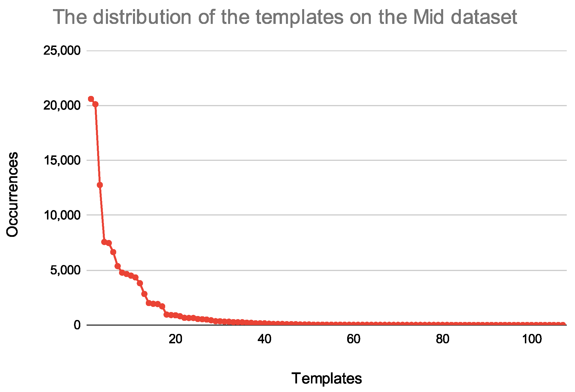
To increase the compression rate of our algorithm, we first examined the properties of our data. We came to the conclusion that our data, which is detailed in Section 5.1, follows the power-law distribution. This can be seen in Figure 2, Figure 3, Figure 4 and Figure 5. The x-axis represents the ordered (based on occurrences) templates from 1 to n, where n is the number of the discovered templates in the dataset.
It can be seen that there are only a few event types with a large number of occurrences and plenty that appear only once or twice. Based on this principle, we decided to assign the IDs based on the repetition of the template. Events with higher frequencies would obtain a smaller ID, which can be stored on fewer bits, while higher IDs would be assigned to rare message types. The IDs are stored as integers with a 32-bit fixed size, that are later encoded using the Huffman coding.
While a parameter of a message type could have more than one value, these values are usually chosen from a finite set of values. To further reduce the size of the compressed log file, we also apply the previously used method to the parameters. A dictionary is created where each parameter value has a unique ID. For example, the parameter “CXP9029630_4” would be stored as ‘1’, where ‘1’ is the ID of the token “CXP9029630_4”. After this, the encoded log file would only contain numbers and spaces.
As a final step, we also employ Huffman coding on the log file. It is a method that is commonly used in data compression and was proposed in [33]. It can be used to create a prefix-free binary code that has a minimum expected codeword length. The algorithm analyses the frequencies of the characters that appear. Commonly appearing symbols would be encoded as shorter bit strings, while uncommon characters are encoded as longer strings. For example, a common symbol such as “a” would be encoded as a single “0”, while rare characters such as “x” would be encoded as “11,000”. The use of Huffman coding is very profitable in our case; since our log file only contains numbers and spaces at this point, we only have to store an additionall fixed-sized Huffman codec, since the alphabet size is always 12 (numbers 0–9, space, and EOF character). The entire IDs are then encoded.
There are three compression models that are widely studied. The first type is where the same model is used for all texts by the static model; this performs badly if the text that was used to build the model and the text to be compressed are different. The second type is the semi-static which works in two runs; a unique model that can be based on occurrence probabilities is built for the text, which is then used to compress the data. The last model is the adaptive model that is initially empty and updates when a new symbol is found [34].
General compressors are not suited for stream-like data, since the compression relies upon the preceding messages and the initial state. Once the template and parameter dictionaries are created, our algorithm is capable of updating them at any time when a new template or parameter is found, which means it can compress stream-like data as well.
Many compression algorithms handle data on a block level. In such cases, it can happen that multiple blocks have to be decompressed to acquire the desired log entry. This can be time-consuming, if we want to use our compressed data for statistical purposes, e.g., to count the number of occurrences of an event type. Since every template gets assigned an ID, our algorithm is capable of decoding any specific log entry without decompressing others. For example, if we want to list all the software updates, we only have to look up the ID of the message type “NPU Software <*> <*>” and decode the parameters that follow the ID. Based on this, it could be said that our algorithm is suited for statistical and analytical use.
We created a script that creates log files with the desired distribution of the message templates. A high-level flow-chart showing how the script works can be seen in Figure 6.
First, a template dictionary, a parameter dictionary, and a dictionary that contains all the possible parameters for each template are created based on the user-provided data. After this, based on the distribution that the user desires, an array is created that contains the probabilities for all of the templates. These are then used to generate a sample list that consists of template IDs that have been generated with the use of the probabilities. In the next step, the desired number of log entries is created as follows. While the sample has items (we iterate through it) the template is chosen based on the actual ID in the sample. Then, each of the tokens in the template is examined. This is performed by iterating over the template and checking if it has a word or the end has been reached. If the token is a wildcard “*”, then it is changed to a randomly chosen parameter from the template’s possible parameters, otherwise, the token is kept. In the end, the log file is generated by writing the created messages to a file.

5. Results

5.1. Data

Our log files were provided by networking appliances that are used at the Ericsson-ELTE Software Technology Lab. To evaluate the effectiveness of the enhanced algorithm compared to the original, we used the same datasets that were used in our previous paper [21], and some new datasets that are several gigabytes in size. All of our datasets are distinct and independent from each other. Each entry of the datasets belongs to one of the 107 possible message types that are used to indicate the runtime information of the networking assets. The distribution of the entries follows the power-law distribution in the case of all investigated datasets. The details of our data, such as the alphabet size or the Shannon Entropy, can be seen Table 1.
The amount of information involved in the value of a random variable is known as Shannon Entropy or Entropy [35]. In the case of a discrete random variable X, that has possible outcomes of x 1 , x 2 , · , x n , that occur with probability P ( x 1 ) , P ( x 2 ) , · , P ( x n ) , the entropy of X is defined as:
H ( X ) = i = 1 n P ( x i ) l o g P ( x i ) ,
where the sum of the variable’s possible values is denoted by ∑. There are other types of entropy, such as k-th order entropy [36].

5.2. Experimental Analysis

We conducted various experiments to demonstrate the compression efficiency of our enhanced algorithm. We also examined the runtime of our algorithm. To obtain a more detailed picture, we compared the compression rate and the speed of our enhanced algorithm with those of general compressors. We investigated whether the compression rate could be further improved with the joint use of our method and general compressors. The time and storage space needed to retrieve all instances of a given set of templates was also investigated. We also compared the compression rates and the memory usage of the proposed algorithm and Logzip, a compressor that also uses hidden structures. The dahuffman python library [37] was used as our Huffman coder. Since Bzip, LZMA, and PPMd are supported by 7-Zip [38], we chose these algorithms as our general compressors. The default settings of 7-Zip were used, which are a 16 MB dictionary size, a word size of 32, and a solid block size of 2 GB. The experimental analyses are divided into six parts and are explained below.

5.2.1. Experiment 1: Comparing the Compression Values Achieved by the Different Enhancements

In order to further improve the compression ratio that our algorithm, proposed in [21], achieved, we employed multiple enhancements. First, we used Huffman coding on the output of the original algorithm, which consisted of an ID and the parameters in string format, for example, “1 CXP9029630_4 R9D3925”, where 1 stands for “NPU Software <*> <*>”. This approach is labeled “Huff”. The second idea was that the template IDs should be assigned based on frequency, and parameters should also be encoded, since the same values appear multiple times, and the average length of a parameter ID is less than the average length of a parameter’s string representation. If “CXP9029630_4” is represented by 1 and “R9D3925” is represented by 2, the output would be “1 1 2”, which is 27 characters less than the original entry. This approach is labeled “Enh”. Finally, we combined the first two ideas. This approach is labeled “Huff”. The compression rates achieved by these enhancements can be seen in Figure 7, Figure 8, Figure 9 and Figure 10.
Based on our experiments, it can be said that each enhancement improves the compression rate. The single use of Huffman coding provides the smallest improvement; the compression rate is around ≈75%, which is ≈17% more than the original algorithm (where the compression rate is 1 minus the ratio of the size of the compressed file to the uncompressed size). The reason behind this is that the lines to be encoded could contain various characters since the parameters are in a plain text format. Due to the large number of possible characters, some of them will have lengthy representations, which results in worse compression capability. The codec size also depends on the number of unique characters. Table 2 contains information about the size of the template dictionary, parameter dictionary, Huffman codec, and the overall compressed data size. WPE stands for “Without Parameter Encoding”. This is used in our second approach, where the parameters are not encoded, only the Huffman coding is used.
It can be seen that the size of the template dictionary is small and constant. In the case of the second enhancement, we were also required to store the parameter dictionary. It is larger than the template dictionary but still negligible compared to the size of the uncompressed data. The use of the parameter dictionary resulted in a ≈80% compression rate, which is ≈20% more than the original algorithm’s. The joint use of the parameter dictionary approach and the Huffman coding provided the best compression rates, around ≈92%. This can be explained by the fact that the file to be compressed only contains numbers and spaces, which results in a constant and small codec. It is also important to mention that this approach scales well for large datasets. In the case of all the enhancements, the MoLFI version has slightly better rates than the one that uses IPLoM.

5.2.2. Experiment 2: Comparing the Speeds of the Different Enhancements

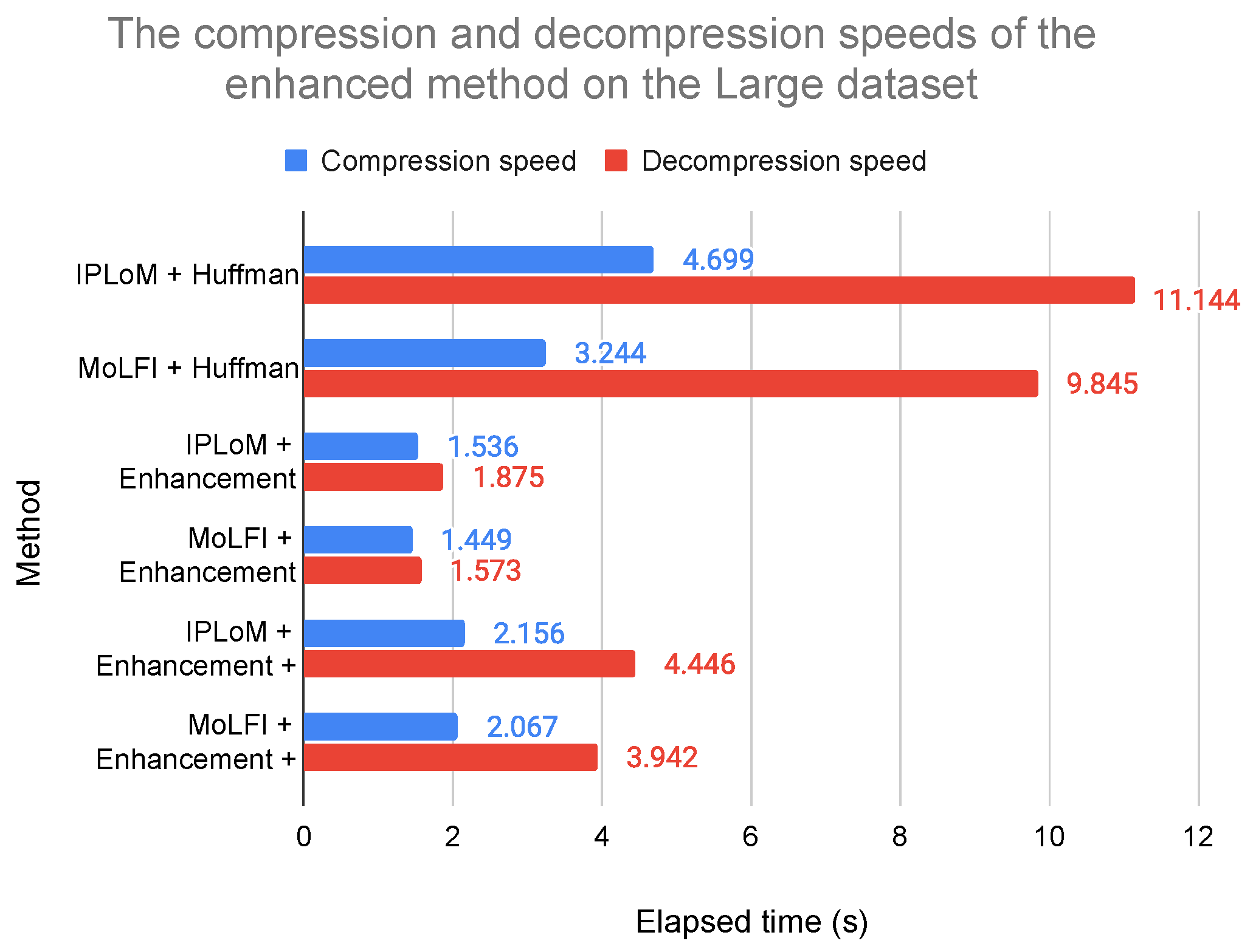
The time it takes for a compressor to compress a file is also an important factor. As a result of this, we found it important to compare the run times of the different enhancements. We also analyzed the time our algorithm took to decompress the data. We assume that the templates are present, so the evaluation of the speed needed to generate the templates is not part of this paper. The results can be seen in Figure 11, Figure 12, Figure 13 and Figure 14.
It can be seen that the creation of a parameter dictionary does not take much time, while the Huffman coding proves to be slower, especially when any kind of character could occur in the file to be compressed, so it takes more time to find the representation in the codec. In the case of the parameter dictionary approach, the decompression time is just slightly more than the time it takes to compress the file. The same cannot be said for the approaches that use Huffman coding, since it takes at least twice as much time to decompress the file when this method is involved. The MoLFI version is somewhat faster than the IPLoM one.

5.2.3. Experiment 3: Comparing the Compression Rates of the New Enhanced Algorithm and General Compressors

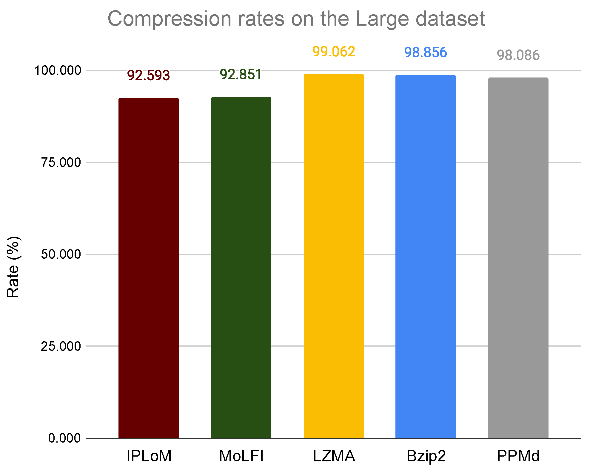
In this experiment, we wanted to compare the compression rate achieved by our parameter dictionary and Huffman coding technique with the compression rates of general compressors. The results can be seen in Figure 15, Figure 16, Figure 17 and Figure 18.
Out of the three investigated general compressors, LZMA has the highest compression rate, with an average of 98.97%, while PPMd has the least, with 97% on average. Our enhanced algorithm achieved 91.49% on average when used with IPLoM and 92.11% in the case of MoLFI. We also wanted to measure the compression rates on larger data, with the size being measured in gigabytes. We only investigated the compression rates of MoLFI, since it had the highest compression rate on the previous datasets. For this purpose, we introduced four new datasets, A, B, C, and D, with the sizes of 2 GB, 5 GB, 10 GB, and 50 GB, respectively. The compression rates achieved are shown in Table 3 and Figure 19, Figure 20, Figure 21 and Figure 22.
It can be seen that, in the case of larger files (with the size of gigabytes), there was no improvement in the compression rate of the examined methods. Bzip2 and PPMd have the best rates, with 95.823% and 94.543%, respectively, while our algorithm falls slightly behind them (approximately 1%). The proposed algorithm also outperforms LZMA with 1.75%.

5.2.4. Experiment 4: Comparing the Speeds of the New Enhanced Algorithm and General Compressors

As mentioned before, the time an algorithm takes to compress the data is also an important measure. As a result of this, we wanted to compare the speeds of the general compressors against our enhanced algorithm. Both the compression and decompression times are analyzed. The time it takes to compress the used datasets are visualized in Figure 23, Figure 24, Figure 25 and Figure 26.
Based on the results, it can be said that general compressors take less time to compress data than our enhanced algorithm. The explanation behind this is that the algorithm has to count and order the templates based on their occurrences, which takes more time than creating a stream of literals or allocating probabilities. It can also be seen that the more log entries that have to be counted, the more time our algorithm takes. Apart from this, we still consider our algorithm to be fast, since it compresses large amounts of data in just a few seconds. In terms of decompression time, our algorithm takes twice as much time as the general compressors, since it has to look up two dictionaries to decode the log messages. Aside from that, our algorithm is slower to decompress than general compressors; it only needs seconds in the case of the investigated datasets. The MoLFI variant of our enhanced algorithm is slightly faster in terms of both compression and decompression.

5.2.5. Experiment 5: Comparing the Compression Rates of the Joint Use of the New Enhanced Algorithm and General Compressors

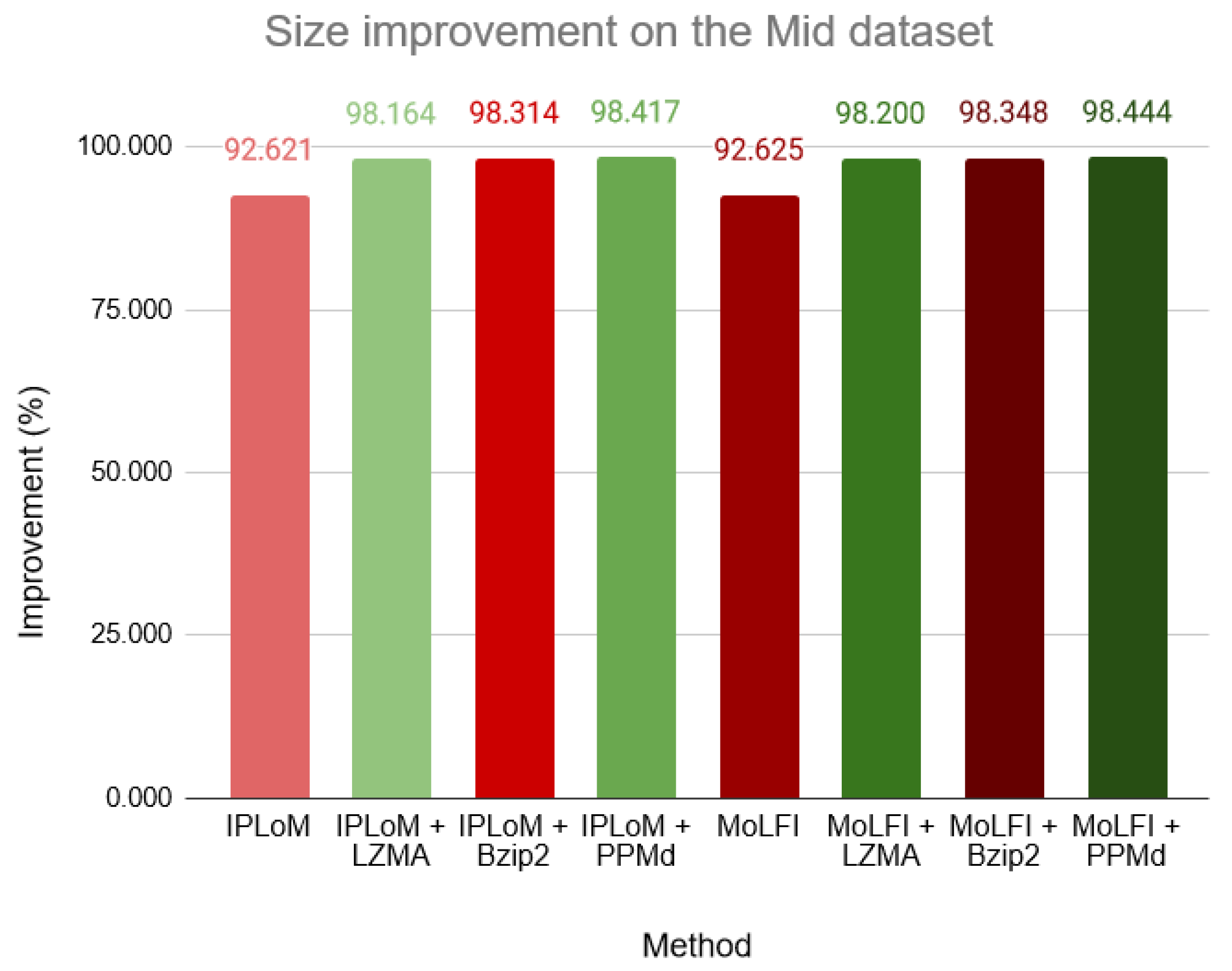
In this experiment, we wanted to investigate if the compression rate can be further improved if we use our enhanced algorithm in conjunction with the general compressors. These compression rates can be seen in Figure 27, Figure 28, Figure 29 and Figure 30.
The use of a general compressor improves the compression rate of our enhanced algorithm by approximately 5%, but this rate still does not reach the compression rate of the single use of general compressors. Nonetheless, we would encourage the use of both our algorithm and traditional compressors, since they can function as a wrapper for our template- and parameter-dictionaries, codec, and compressed file. Out of the tried combinations, the MoLFI variant of our enhanced algorithm used alongside PPMd had the best compression rate with an average of 98.42%.
We also wanted to investigate the compression rate of the joint use of the MoLFI version (since it has better rates) of our proposed method and general compressors on the previously mentioned datasets, A, B, C, and D. The results are shown in Figure 31, Figure 32, Figure 33 and Figure 34.
It can be seen that, in the case of datasets with sizes in gigabytes, the joint use produces approximately 1% higher compression rates than the ones achieved by the single use of the general compressor in Section 5.2.3.

5.2.6. Experiment 6: Comparing the Speeds of the Joint Use of the New Enhanced Algorithm and General Compressors

We also evaluated the compression and decompression times of the joint use of our algorithm and general compressors. The results can be seen in Figure 35, Figure 36, Figure 37 and Figure 38.
The use of a general compressor increases both the compression and decompression; however, this extra time is negligible. In terms of compression, out of all combinations, the joint use of MoLFI and PPMd proved to be the fastest, while the combination of MoLFI and LZMA takes less time to decompress the data. The use of any combination is considered to be fast.

5.2.7. Experiment 7: Comparing the Speeds and the Storage Sizes Needed to Retrieve All Instances of an Event Type by the New Enhanced Algorithm and General Compressors

In this experiment, we randomly selected 10 and 100 templates and investigated the time and storage space that were needed to recover all log entries that correspond to a template in the set. For this experiment, the previously introduced A dataset was used. Figure 39 and Figure 40 show the results of the experiment.
Since we can find the corresponding log entry based on the ID of the template, in the case of our algorithm, only the Huffman decoding step is necessary. This requires more time than decompressing with a general compressor; however, the time needed to look up the entries is considerably less. The reason behind this is that we only need to check the first n characters of the encoded file (where n is the length of the ID), rather than checking all the constant tokens. The storage size needed is much larger in the case of general compressors, since a full decompression of the data is necessary to look for templates, while, in the case of our algorithm, the intermediate compressed file is enough. In the case of dataset A, this means 2 GB for the general compressors, while only 290 MB for our algorithm.
We also wanted to measure the time needed to retrieve the entries when our algorithm is used in conjunction with a general compressor. Since, in Section 5.2.5, the joint use of the proposed method and PPMd had the best compression rate, we chose PPMd as the general compressor for this experiment. The compressed file is first decompressed with PPMd, then the compressed file is decoded using the Huffman algorithm. The results can be seen in Figure 41 and Figure 42.
It can be seen that the decompression time increases with the time taken by the PPMd to decompress the dictionaries and the compressed file generated by our algorithm, but it can still quickly recover the entries corresponding to the randomly selected templates. There is no difference in the space required to lookup the entries.

5.2.8. Experiment 8: The Comparison of the Compression Rates Achieved by the Proposed Algorithm and Logzip

It is also important to compare the compression rates of the proposed method and other algorithms that use the same approach. Like our algorithm, Logzip [19] also utilizes hidden structures (templates) to reduce the size of a file. It also uses the general compressor Bzip2 to further decrease the size. In this experiment, we compare the achieved compression rates in the case of the previously mentioned datasets, A, B, and C. The results can be seen in Figure 43.
Our method has a compression rate that is approximately 1% higher than Logzip’s. In contrast with Logzip, our algorithm does not incorporate the use of general algorithms. With the joint use, our method could achieve higher rates as explained in Section 5.2.5.

5.2.9. Experiment 9: Investigating the Memory Usage of the Proposed Algorithm and Logzip

Memory usage is a significant aspect of a compressor, so we investigated the average and maximum memory usages of the proposed algorithm and Logzip [19]. We also measured the duration of time that the compressors used the memory for. Dataset A was used to conduct the experiment. The computer which was used to perform the measurements had 16 GB of DDR4 RAM. The results are shown in Figure 44.
It can be seen that our algorithm uses 44% less memory on average, and the maximum memory used is 2.9 times less than in the case of Logzip. This could be explained by the loading method of the messages. While our algorithm reads lines after each other (similar to when messages come in a stream), Logzip loads the whole file into a dataframe that is located in the memory. Furthermore, Logzip consumes the memory for four times as long as the proposed algorithm. It can be noticed that the memory usage scales with the size of the input. The available memory has to be at least 2.2 times the input size.

5.2.10. Experiment 10: Generating Log Messages with Different Distributions and Evaluating the Compression Rates

In the final experiment, we investigated whether our enhanced algorithm had high compression rates even in the case of distributions other than the power law. We created four datasets, which were different in size and distribution. While generating the “random” datasets, each template had a 5% probability to be created by the sampling algorithm. We created a file that consisted of 1 million entries and a file that consisted of 50 million entries based on this principle. The generation of the other two datasets was similar, except that, in this case, normal distribution was used instead of equal 5% probabilities. The distribution of the templates in the case of the generated files can be seen in Figure 45, Figure 46, Figure 47 and Figure 48.
After the creation of the custom datasets, we measured the compression rates of our enhanced algorithm. The results are shown in Figure 49.
It can be seen that our algorithm is capable of achieving high compression rates regardless of the distribution of the templates. In the case of all the datasets, at least a 94% compression rate was achieved, which indicates the compressing capacity of our algorithm.

6. Discussion and Conclusions

In this paper, we evaluated the compression capacity of an enhanced version of the algorithm that we proposed in [21]. The original algorithm uses template miners to identify the templates. Based on the templates, a dictionary is created where each ID represents an event type. The log lines are then represented using the corresponding ID and parameter list. Using this approach, we were able to achieve around 67% compression rates. To improve this performance, we introduced several enhancements to the algorithm in this paper. First, the templates were ordered based on the number of their occurrences. Smaller IDs were assigned to the more frequent templates. As a second step, we created a dictionary for the templates in a similar manner. This resulted in encoded log messages that only contained numbers. Finally, Huffman coding was used to further compress the file.
To analyze the performance of the enhanced algorithm, we conducted several experiments. The experimental results showed that each enhancement improved the compression capacity. The joint use of the parameter dictionary and Huffman coding achieved an average of 92% compression rate, which is 25% more than the original algorithm. In terms of speed, we consider our algorithm to be fast, since it only takes seconds to compress and decompress the investigated log files. We also compared our algorithm with general compressors. While general compressors are faster and achieve better compression rates, around 98%, they are not well suited for statistical applications. With the use of our algorithm, statistical questions such as ‘What is the distribution of the templates?’ or ‘What is the frequency of the different parameters of a message type?’ can easily be answered. The instances of given templates can also be found faster than in the case of general compressors.
Based on our experiment we would suggest the joint use of our algorithm and general compressors, since it improves the compression rates and functions as a wrapper for the created templates and the encoded file.
We only evaluated the performance on static log files, it would be beneficial to measure the compression rate, speed, and memory usage in the case of stream-like data. It would be also interesting to compare the performance of our method with the performance of other general compressors. We also want to investigate the connection between the compression rate and the k-th order empirical entropy.

Author Contributions

Conceptualization, P.M., P.L.-K. and A.K.; methodology, P.M., P.L.-K. and A.K.; software, P.M. and P.L.-K.; validation, P.M., P.L.-K. and A.K.; investigation, P.M., P.L.-K. and A.K.; writing–original draft preparation, P.M., P.L.-K. and A.K.; writing–review and editing, P.M., P.L.-K. and A.K.; supervision, A.K.; project administration, A.K. All authors have read and agreed to the published version of the manuscript.

Funding

The project has been supported by grants from the “Application Domain Specific Highly Reliable IT Solutions” project that has been implemented with the support provided from the National Research, Development, and Innovation Fund of Hungary, financed under the Thematic Excellence Program TKP2020-NKA-06 (National Challenges Subprogram) funding scheme.

Institutional Review Board Statement

Not applicable.

Informed Consent Statement

Not applicable.

Data Availability Statement

The data was provided by the Ericsson-ELTE Software Technology Lab.

Acknowledgments

This publication is the partial result of the Research and Development Operational Program for the project “Modernisation and Improvement of Technical Infrastructure for Research and Development of J. Selye University in the Fields of Nanotechnology and Intelligent Space”, ITMS 26210120042, co-funded by the European Regional Development Fund and supported by the ÚNKP-21-3 New National Excellence Program of the Ministry for Innovation and Technology from the source of the National Research, Development, and Innovation Fund. The project was also supported by the Ericsson-ELTE Software Technology Lab.

Conflicts of Interest

The authors declare no conflict of interest.

Abbreviations

The following abbreviations are used in this manuscript:
IPLoMIterative Partitioning Log Mining
MoLFIMulti-objective Log message Format Identification
NSGA-IINon-dominated Sorting Genetic Algorithm II
BWTBurrows–Wheeler Transformation
LZMALempel–Ziv–Markov-chain Algorithm
PPMPrediction by Partial Matching
EnhEnhanced version of our algorithm
HuffHuffman coding
WPEWithout Parameter Encoding

References

  1. Landauer, M.; Wurzenberger, M.; Skopik, F.; Settanni, G.; Filzmoser, P. Dynamic log file analysis: An unsupervised cluster evolution approach for anomaly detection. In Computers & Security; Elsevier: Amsterdam, The Netherlands, 2018; Volume 79, pp. 94–116. [Google Scholar] [CrossRef]
  2. Aivalis, C.; Boucouvalas, A.C. Log File Analysis of E-commerce Systems in Rich Internet Web 2.0 Applications. In Proceedings of the PCI 2011—15th Panhellenic Conference on Informatics, Kastoria, Greece, 30 September–2 October 2011; Volume 10, pp. 222–226. [Google Scholar] [CrossRef]
  3. Nagaraj, K.; Killian, C.; Neville, J. Structured comparative analysis of systems logs to diagnose performance problems. In Proceedings of the 9th USENIX Symposium on Networked Systems Design and Implementation, Jan Jose, CA, USA, 25–27 April 2012; pp. 353–366. [Google Scholar]
  4. Logothetis, D.; Trezzo, C.; Webb, K.C.; Yocum, K. In-situ MapReduce for log processing. In Proceedings of the USENIX ATC, Portland, OR, USA, 14–15 June 2011; Volume 11, p. 115. [Google Scholar]
  5. Li, H.; Shang, W.; Hassan, A.E. Which log level should developers choose for a new logging statement? In Empirical Software Engineering; Springer: New York, NY, USA, 2017; Volume 22, pp. 1684–1716. [Google Scholar] [CrossRef]
  6. Lin, H.; Zhou, J.; Yao, B.; Guo, M.; Li, J. Cowic: A column-wise independent compression for log stream analysis. In Proceedings of the 2015 15th IEEE/ACM International Symposium on Cluster, Cloud and Grid Computing, Shenzhen, China, 4–7 May 2015; pp. 21–30. [Google Scholar] [CrossRef]
  7. Yao, K.; Li, H.; Shang, W.; Hassan, A.E. A study of the performance of general compressors on log files. In Empirical Software Engineering; Springer: New York, NY, USA, 2020; Volume 25, pp. 3043–3085. [Google Scholar] [CrossRef]
  8. Du, M.; Li, F. Spell: Streaming parsing of system event logs. In Proceedings of the 2016 IEEE 16th International Conference on Data Mining, Barcelona, Spain, 12–15 December 2016; pp. 859–864. [Google Scholar] [CrossRef]
  9. Shima, K. Length matters: Clustering system log messages using length of words. arXiv 2016, arXiv:1611.03213. [Google Scholar]
  10. He, P.; Zhu, J.; Zheng, Z.; Lyu, M.R. Drain: An online log parsing approach with fixed depth tree. In Proceedings of the 2017 IEEE International Conference on Web Services (ICWS), Honolulu, HI, USA, 25–30 June 2017; pp. 33–40. [Google Scholar] [CrossRef]
  11. Christensen, R.; Li, F. Adaptive log compression for massive log data. In Proceedings of the SIGMOD Conference, New York, NY, USA, 22–27 June 2013; pp. 1283–1284. [Google Scholar]
  12. Feng, B.; Wu, C.; Li, J. MLC: An efficient multi-level log compression method for cloud backup systems. In Proceedings of the 2016 IEEE Trustcom/BigDataSE/ISPA, Tianjin, China, 23–26 August 2016; pp. 1358–1365. [Google Scholar] [CrossRef]
  13. Mell, P.; Harang, R.E. Lightweight packing of log files for improved compression in mobile tactical networks. In Proceedings of the 2014 IEEE Military Communications Conference, Baltimore, MD, USA, 6–8 October 2014; pp. 192–197. [Google Scholar] [CrossRef]
  14. Grabowski, S.; Deorowicz, S. Web log compression. Automatyka/Akademia Górniczo-Hutnicza im. Stanisława Staszica w Krakowie 2007, 11, 417–424. [Google Scholar]
  15. Lloyd, T.; Barton, K.; Tiotto, E.; Amaral, J.N. Run-length base-delta encoding for high-speed compression. In Proceedings of the 47th International Conference on Parallel Processing Companion, Eugene, OR, USA, 13–16 August 2018; pp. 1–9. [Google Scholar] [CrossRef]
  16. Tan, H.; Zhang, Z.; Zou, X.; Liao, Q.; Xia, W. Exploring the Potential of Fast Delta Encoding: Marching to a Higher Compression Ratio. In Proceedings of the 2020 IEEE International Conference on Cluster Computing (CLUSTER), Kobe, Japan, 14–17 September 2020; pp. 198–208. [Google Scholar] [CrossRef]
  17. Skibiński, P.; Swacha, J. Fast and efficient log file compression. In Proceedings of the CEUR Workshop, 11th East-European Conference on Advances in Databases and Information Systems, Varna, Bulgaria, 29 September–3 October 2007; pp. 56–69. [Google Scholar]
  18. Otten, F.; Irwin, B.; Thinyane, H. Evaluating text preprocessing to improve compression on maillogs. In Proceedings of the 2009 Annual Research Conference of the South African Institute of Computer Scientists and Information Technologists, Emfuleni, South Africa, 12–14 October 2009; pp. 44–53. [Google Scholar] [CrossRef]
  19. Liu, J.; Zhu, J.; He, S.; He, P.; Zheng, Z.; Lyu, M.R. Logzip: Extracting hidden structures via iterative clustering for log compression. In Proceedings of the 2019 34th IEEE/ACM International Conference on Automated Software Engineering (ASE), San Diego, CA, USA, 11–15 November 2019; pp. 863–873. [Google Scholar] [CrossRef] [Green Version]
  20. Hätönen, K.; Boulicaut, J.F.; Klemettinen, M.; Miettinen, M.; Masson, C. Comprehensive log compression with frequent patterns. In International Conference on Data Warehousing and Knowledge Discovery; Springer: Berlin/Heidelberg, Germany, 2003; pp. 360–370. [Google Scholar] [CrossRef] [Green Version]
  21. Marjai, P.; Lehotay-Kéry, P.; Kiss, A. The Use of Template Miners and Encryption in Log Message Compression. Computers 2021, 10, 83. [Google Scholar] [CrossRef]
  22. He, P.; Zhu, J.; He, S.; Li, J.; Lyu, M.R. An evaluation study on log parsing and its use in log mining. In Proceedings of the 2016 46th Annual IEEE/IFIP International Conference on Dependable Systems and Networks, Toulouse, France, 28 June–1 July 2016; pp. 654–661. [Google Scholar] [CrossRef]
  23. Makanju, A.; Zincir-Heywood, A.N.; Milios, E.E. A lightweight algorithm for message type extraction in system application logs. IEEE Trans. Knowl. Data Eng. 2011, 24, 1921–1936. [Google Scholar] [CrossRef]
  24. Messaoudi, S.; Panichella, A.; Bianculli, D.; Briand, L.; Sasnauskas, R. A search-based approach for accurate identification of log message formats. In Proceedings of the 26th Conference on Program Comprehension, Gothenburg, Sweden, 27 May–3 June 2018; pp. 167–177. [Google Scholar] [CrossRef] [Green Version]
  25. Deb, K.; Pratap, A.; Agarwal, S.; Meyarivan, T.A.M.T. A fast and elitist multiobjective genetic algorithm: NSGA-II. IEEE Trans. Evol. Comput. 2002, 6, 182–197. [Google Scholar] [CrossRef] [Green Version]
  26. Sivanandam, S.N.; Deepa, S.N. Genetic algorithms. In Introduction to Genetic Algorithms; Springer: Berlin/Heidelberg, Germany, 2008; pp. 15–37. [Google Scholar] [CrossRef]
  27. Syswerda, G. Uniform crossover in genetic algorithms. In Proceedings of the Third International Conference on Genetic Algorithms; Morgan Kaufmann Publishers: Burlington, MA, USA, 1989; pp. 2–9. [Google Scholar]
  28. Branke, J.; Deb, K.; Dierolf, H.; Osswald, M. Finding knees in multi-objective optimization. In International Conference on Parallel Problem Solving from Nature; Springer: Berlin/Heidelberg, Germany, 2004; pp. 722–731. [Google Scholar]
  29. Burrows, M.; Wheeler, D. A block-sorting lossless data compression algorithm. In Digital SRC Research Report; Digital Systems Research Center: Palo Alto, CA, USA, 1994. [Google Scholar]
  30. Ziv, J.; Lempel, A. A universal algorithm for sequential data compression. IEEE Trans. Inf. Theory 1977, 23, 337–343. [Google Scholar] [CrossRef] [Green Version]
  31. Bell, T.; Witten, I.H.; Cleary, J.G. Modeling for text compression. ACM Comput. Surv. 1989, 21, 557–591. [Google Scholar] [CrossRef]
  32. Cleary, J.; Witten, I. Data compression using adaptive coding and partial string matching. IEEE Trans. Commun. 1984, 32, 396–402. [Google Scholar] [CrossRef] [Green Version]
  33. Huffman, D.A. A method for the construction of minimum-redundancy codes. Proc. IRE 1952, 40, 1098–1101. [Google Scholar] [CrossRef]
  34. Moffat, A.; Zobel, J.; Sharman, N. Text compression for dynamic document databases. IEEE Trans. Knowl. Data Eng. 1997, 9, 302–313. [Google Scholar] [CrossRef] [Green Version]
  35. Shannon, C.E. A mathematical theory of communication. Bell Syst. Tech. J. 1948, 27, 379–423. [Google Scholar] [CrossRef] [Green Version]
  36. Ferragina, P.; González, R.; Navarro, G.; Venturini, R. Compressed text indexes: From theory to practice. J. Exp. Algorithm. 2009, 13, 1.12–1.31. [Google Scholar] [CrossRef]
  37. Dahuffman Python Library. Available online: https://pypi.org/project/dahuffman/ (accessed on 22 September 2021).
  38. 7-Zip. Available online: https://www.7-zip.org/ (accessed on 1 October 2021).
Figure 1. Excerpt of log file generated by real-world networking device.
Applsci 12 02044 g001
Figure 2. Distribution of the templates in the Small dataset.
Applsci 12 02044 g002
Figure 3. Distribution of the templates in the Mid dataset.
Applsci 12 02044 g003
Figure 4. Distribution of the templates in the Large dataset.
Applsci 12 02044 g004
Figure 5. Distribution of the templates in the Big dataset.
Applsci 12 02044 g005
Figure 6. The flow chart that represents log data generation.
Applsci 12 02044 g006
Figure 7. Compression rate of the different enhancement approaches of the Small dataset.
Applsci 12 02044 g007
Figure 8. Compression rate of the different enhancement approaches of the Mid dataset.
Applsci 12 02044 g008
Figure 9. Compression rate of the different enhancement approaches of the Large dataset.
Applsci 12 02044 g009
Figure 10. Compression rate of the different enhancement approaches of the Big dataset.
Applsci 12 02044 g010
Figure 11. Speeds of the different enhancements used on the Small dataset.
Applsci 12 02044 g011
Figure 12. Speeds of the different enhancements used on the Mid dataset.
Applsci 12 02044 g012
Figure 13. Speeds of the different enhancements used on the Large dataset.
Applsci 12 02044 g013
Figure 14. Speeds of the different enhancements used on the Big dataset.
Applsci 12 02044 g014
Figure 15. The comparison of compression rates of the enhanced algorithm and general compressors on the Small dataset.
Applsci 12 02044 g015
Figure 16. The comparison of compression of the enhanced algorithm and general compressors on the Mid dataset.
Applsci 12 02044 g016
Figure 17. The comparison of compression rates of the enhanced algorithm and general compressors on the Large dataset.
Applsci 12 02044 g017
Figure 18. The comparison of compression rates of the enhanced algorithm and general compressors on the Big dataset.
Applsci 12 02044 g018
Figure 19. The comparison of compression rates of the enhanced algorithm and general compressors on the A dataset.
Applsci 12 02044 g019
Figure 20. The comparison of compression of the enhanced algorithm and general compressors on the B dataset.
Applsci 12 02044 g020
Figure 21. The comparison of compression rates of the enhanced algorithm and general compressors on the C dataset.
Applsci 12 02044 g021
Figure 22. The comparison of compression rates of the enhanced algorithm and general compressors on the D dataset.
Applsci 12 02044 g022
Figure 23. The speeds of the enhanced algorithm and general compressors on the Small dataset.
Applsci 12 02044 g023
Figure 24. The speeds of the enhanced algorithm and general compressors on the Mid dataset.
Applsci 12 02044 g024
Figure 25. The speeds of the enhanced algorithm and general compressors on the Large dataset.
Applsci 12 02044 g025
Figure 26. The speeds of the enhanced algorithm and general compressors on the Big dataset.
Applsci 12 02044 g026
Figure 27. The compression rates of the joint use on the Small dataset.
Applsci 12 02044 g027
Figure 28. The compression rates of the joint use on the Mid dataset.
Applsci 12 02044 g028
Figure 29. The compression rates of the joint use on the Large dataset.
Applsci 12 02044 g029
Figure 30. The compression rates of the joint use on the Big dataset.
Applsci 12 02044 g030
Figure 31. The compression rates of the joint use on the A dataset.
Applsci 12 02044 g031
Figure 32. The compression rates of the joint use on the B dataset.
Applsci 12 02044 g032
Figure 33. The compression rates of the joint use on the C dataset.
Applsci 12 02044 g033
Figure 34. The compression rates of the joint use on the D dataset.
Applsci 12 02044 g034
Figure 35. The speeds of the joint use on the Small dataset.
Applsci 12 02044 g035
Figure 36. The speeds of the joint use on the Mid dataset.
Applsci 12 02044 g036
Figure 37. The speeds of the joint use on the Large dataset.
Applsci 12 02044 g037
Figure 38. The speeds of the joint use on the Big dataset.
Applsci 12 02044 g038
Figure 39. The times needed to recover all instances of the 10 template.
Applsci 12 02044 g039
Figure 40. The times needed to recover all instances of the 100 template.
Applsci 12 02044 g040
Figure 41. The times needed to recover all instances of the 10 template in case of the joint compression.
Applsci 12 02044 g041
Figure 42. The times needed to recover all instances of the 100 template in case of the joint compression.
Applsci 12 02044 g042
Figure 43. The compression rates achieved by our method and Logzip on datasets A B and C.
Applsci 12 02044 g043
Figure 44. The memory usage of the proposed method and Logzip.
Applsci 12 02044 g044
Figure 45. The template distribution of the 1 million randomly generated messages dataset.
Applsci 12 02044 g045
Figure 46. The template distribution of the 50 million randomly generated messages dataset.
Applsci 12 02044 g046
Figure 47. The template distribution of the 1 million messages dataset generated based on normal distribution.
Applsci 12 02044 g047
Figure 48. The template distribution of the 50 million messages dataset generated based on normal distribution.
Applsci 12 02044 g048
Figure 49. The compression rates achieved by our method on the generated datasets.
Applsci 12 02044 g049
Table 1. Size of the datasets.
NameNumber of MessagesSize in KilobytesAlphabet SizeShannon Entropy
Small39,1391152 KB765.08167
Mid124,4334607 KB765.08872
Large280,00210,198 KB745.05287
Big637,36922,840 KB715.00206
A50,000,0002,039,483 KB764.97789
B130,000,0005,303,394 KB764.97798
C254,000,00010,361,437 KB764.97781
D1,264,000,00051,562,601 KB764.89284
Table 2. Size of the different assets.
IPLoMSmall DatasetMid DatasetLarge DatasetBig Dataset
Huff
Template dictionary2.981 KB4.266 KB4.24 KB4.293 KB
Huffman codec (WPE)1.158 KB1.179 KB1.203 KB1.197 KB
Compressed file409.426 KB1068.173 KB2674.835 KB5776.537 KB
Overall413.565 KB1073.618 KB2680.278 KB5782.027 KB
Enh
Template dictionary2.981 KB4.266 KB4.24 KB4.293 KB
Parameter dictionary6.877 KB22.151 KB24.906 KB25.626 KB
Compressed file358.361 KB855.013 KB2004.595 KB4506.784 KB
Overall368.219 KB881.43 KB2033.741 KB4536.703 KB
Enh Huff
Template dictionary2.981 KB4.266 KB4.24 KB4.293 KB
Parameter dictionary6.877 KB22.151 KB24.906 KB25.626 KB
Huffman codec0.362 KB0.362 KB0.362 KB0.362 KB
Compressed file132.147 KB306.09 KB725.813 KB1608.534 KB
Overall142.367 KB332.869 KB755.321 KB1638.815 KB
MoLFISmall DatasetMid DatasetLarge DatasetBig Dataset
Huff
Template dictionary3.832 KB4.45 KB4.606 KB4.461 KB
Huffman codec (WPE)1.068 KB1.125 KB1.118 KB1.134 KB
Compressed file313.133 KB986.065 KB2455.239 KB5550.092 KB
Overall318.033 KB991.64 KB2460.963 KB5555.687 KB
Enh
Template dictionary3.832 KB4.45 KB4.606 KB4.461 KB
Parameter dictionary6.348 KB21.743 KB24.448 KB25.206 KB
Compressed file288.102 KB854.308 KB1996.157 KB4522.154 KB
Overall298.282 KB880.501 KB2025.211 KB4551.821 KB
Enh Huff
Template dictionary3.832 KB4.45 KB4.606 KB4.461 KB
Parameter dictionary6.348 KB21.743 KB24.448 KB25.206 KB
Huffman codec0.362 KB0.362 KB0.362 KB0.362 KB
Compressed file105.48 KB303.202 KB699.61 KB1606.879 KB
Overall116.022 KB329.757 KB729.026 KB1636.908 KB
Table 3. Compression rates on the A, B, C and D datasets.
DatasetProposedLZMABzip2PPMd
A94.652%92.931%95.823%95.542%
B94.782%92.931%95.823%95.543%
C94.650%92.932%95.823%95.543%
D94.682%92.931%95.823%95.543%
Publisher’s Note: MDPI stays neutral with regard to jurisdictional claims in published maps and institutional affiliations.