Abstract
Burrs form due to the plastic deformation of materials during machining processes, such as milling and drilling. Deburring can be very difficult when the burrs are not easily accessible for removal. In this study, abrasive flow machining (AFM) was adopted for deburring the edges of milling specimens. Based on the experimental observations on AL6061 specimens, the deburring performance was characterized in terms of flow speed, the local curvature of the streamline near the burr edge, and shear stress. A new objective function that can predict the extent of deburring is proposed based on these characteristics and validated through milling burr edge erosion tests by abrasive flow. Based on the assumption that the flow component is tangential to the burr edge has relatively little contribution to the edge erosion, an attempt was made for the application of the new objective function to the three-dimensional burr edge formed by two intersecting holes drilled with offset. The deburring test results and predictions from three-dimensional computational fluid dynamics’ (CFD) simulations were in reasonable agreement.
1. Introduction
Burrs are formed due to the plastic deformation of materials during machining processes, such as milling and drilling. When they occur in places with poor accessibility, deburring can be very difficult. Burrs reduce the precision of products, hinder assembly operations, and lead to expensive post-processing costs [1]. If burrs on components fall off during operation, it can cause problems during machining and result in downtime.
Several studies have been performed on deburring tools and processes, such as steel wire brushes, hand tools, electrochemical machining, abrasive ultrasonic machining, abrasive jet machining with air or water, thermal impulse deburring, and suction-based abrasive flow control [2,3,4,5,6,7,8,9]. Each of these deburring methods has its own merits and disadvantages and can be improved further. For example, deburring microfluidic channels with a stainless steel wire brush might seem a relatively simple process. However, damage to the workpiece beyond the burr zone is inevitable. As for electrochemical machining, difficulties with the burr edge accessibility can be alleviated, but the formation of large burrs, in addition to the difficulties faced in precision control of machining depth and high cost, is a challenge.
Abrasive flow machining (AFM) has been mainly used for polishing and deburring [10,11]. Dixit classified AFM techniques into one-way, two-way, multi-way, and orbital processes [12]. These AFM processes employ a high-viscosity medium, incurring a high-drive load [13]. This limits its applications to low-speed flow and relatively simple workpiece geometries. Attempts have been made to apply AFM to a low-viscosity abrasive medium for high-speed and complex workpiece geometries [14,15,16,17]. For milling burrs, Kim suggested that an objective function should be applied to the design of flow guides and experimentally verify the deburring performance [18]. The suggested objective function includes the effect of flow intensity near the burr edge in terms of wall shear stress and the effect of streamline curvature near the burr edge, characterizing the flow pathlines brushing through the burrs.
In this study, the effect of flow speed on deburring near the burr edge was investigated in addition to the local shear stress and streamline curvature suggested by [18]. Based on the preliminary deburring tests on milling specimens of AL6061, an updated objective function is proposed and verified through experiments. Based on this new objective function, the deburring performance on intersecting holes with offset was predicted and confirmed through experiments.
2. Abrasive Flow Machining
2.1. Deburring Mechanism
According to the study of Ulman, deburring by abrasive flow progresses in three major steps [19]. First, burrs are forced to bend in one or two directions and cracks may initiate at the roots. Second, the cracks ultimately cause large burrs to fall off due to fatigue failure. Finally, the remaining burrs wear off to rounded or chamfered edges. As the burrs disappear and flow resistance decreases, the material removal rate also decreases on nearing the completion of the process.
Chen and Edward conducted studies on elbow erosion by abrasive flow. According to these studies, the location where the streamlines hurtle against the wall of the elbow pipe coincides with the region wherein a lot of erosion occurs in real [20,21].
In addition, Wong reported that erosion occurs when the direction of abrasive flow is suddenly changed [22]. In the study of Kwon, it was suggested that the shear stress at the burr edge caused by abrasive flow has a great effect on the deburring performance [9].
2.2. Objective Function
Kim reported that shear stress is an important factor in the deburring mechanism [18]. It was also reported that a smaller local curvature of the streamlines near the burr edge is more favorable for momentum transfer from the abrasive particles to the burr edge. Based on this principle, an objective function was proposed for characterizing deburring performance as follows:
here, fob,Kim is the objective function suggested by Kim et al., τxy and κ are the local wall shear stress and streamline curvature in the vicinity of the burr edge [18].
3. Preliminary Testing
3.1. Deburring System
Figure 1 is a schematic diagram of the system used in this study for the deburring experiment. Two concentric hydraulic cylinders and pistons were coupled to a drive point connected to a linear actuator for reciprocating motion. The cylinders were connected to the specimen by hoses to accommodate the abrasive flow medium. A disposable protrusion with the burr edge prepared by milling was assembled in the middle of the specimen.
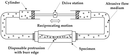
Figure 1.
Schematic diagram of the abrasive flow deburring system with the specimen.
The specimen was made of AL6061, with dimensions of 120 mm × 40 mm × 35 mm, as shown in Figure 2. The side inlets were machined by a 12 mm drill for hose fittings. A fluid channel with 1.5 mm width and 3 mm depth was machined on the top face. In the middle of the channel, a disposable protrusion with 4.25 mm length was assembled into a recess, leaving a 1 mm local gap, as shown in Figure 3.

Figure 2.
Specimen for preliminary testing.
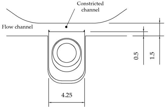
Figure 3.
Dimensions of the protrusion with the burr edges (in mm).
The definition of flow length L is given by
where VF is the total flow volume of the abrasive medium, and A is the local cross-sectional area of the flow path above the protrusion with 1 mm width and 3 mm depth.
3.2. Test Setup (System and Abrasive Flow Medium)
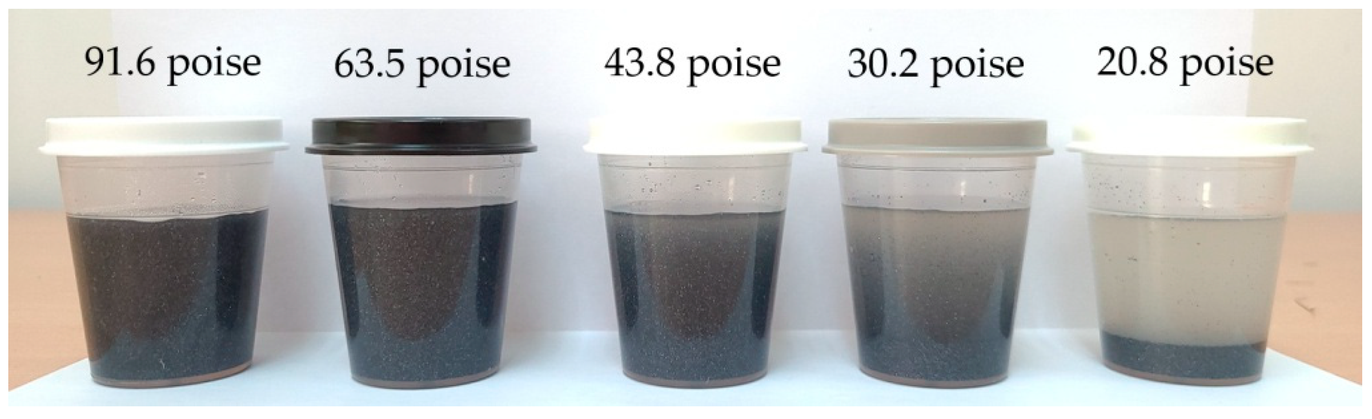
An abrasive flow medium contains abrasive particles, a viscosity controlling agent, and a base fluid. Low-flow speed and low viscosity may cause sedimentation while high-flow speed and high viscosity may overload the deburring system. Practical ranges of flow speed and viscosity were identified through two-stage testing. First, the static sedimentation test was performed for a set of media with different viscosities. Second, for the selected viscosity range, system drive tests were performed at various flow speeds with reference to the constricted channel above the protrusion. The tests were carried out on abrasive particles of grain size #100.
In the static test, the abrasive flow media were sealed in plastic containers and observed for 72 h to monitor sedimentation. As shown in Figure 4, sedimentation was observed below 43.8 poise.
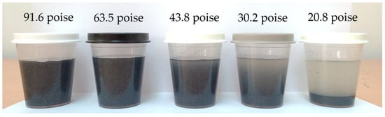
Figure 4.
Results of the static sedimentation test for abrasive fluids with different viscosities after 72 h (from left to right—91.6, 63.5, 43.8, 30.2, and 20.8 poise).
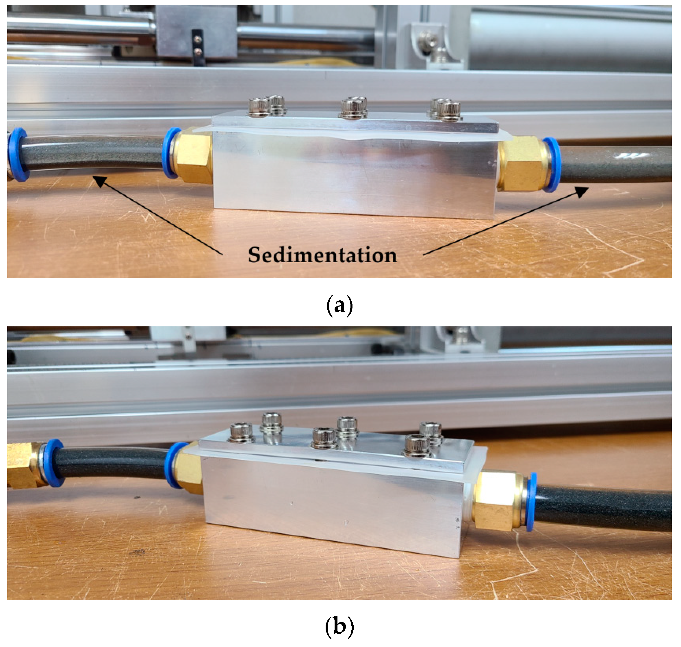
In the dynamic sedimentation test, the transparent hoses were monitored for 2 h of the deburring system operation with a preliminary specimen. As seen in Figure 5a, it was possible to visually identify sedimentation. As listed in Table 1, the viscosity without sedimentation, with the widest speed range, was 43.8 poise. It was confirmed that the selected 43.8 poise fluid was operable at flow speeds of 4.5 m/s and 6.7 m/s.
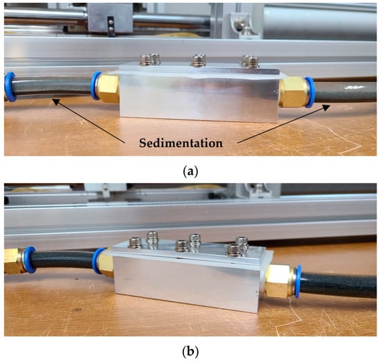
Figure 5.
Visual monitoring of sedimentation in the transparent connection hoses: (a) sedimentation; (b) no sedimentation.

Table 1.
Dynamic sedimentation test results for different viscosity and flow speed combinations.
3.3. 200 km Flow Length Test and Results
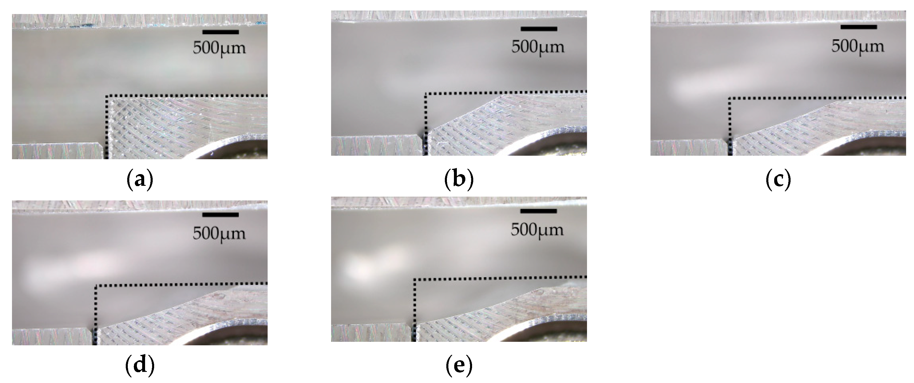
For investigating the effects of flow speed and flow length on deburring, the flow length (L) was fixed at 200 km and the 43.8 poise medium was used. The progress of deburring was recorded at every 50 km of flow length. Figure 6 shows the deburred edges at the flow speed of 7.8 m/s. The dotted lines represent the burr-free boundaries이 s of the specimen before deburring. It is evident that the flow length has a significant effect on edge erosion. Moreover, the erosion exceeded far beyond deburring at the flow length of 50 km.

Figure 6.
Progress of burr edge erosion for the flow speed of V = 7.8 m/s at every 50 km of flow length: (a) 0 km; (b) 50 km; (c) 100 km; (d) 150 km; (e) 200 km.
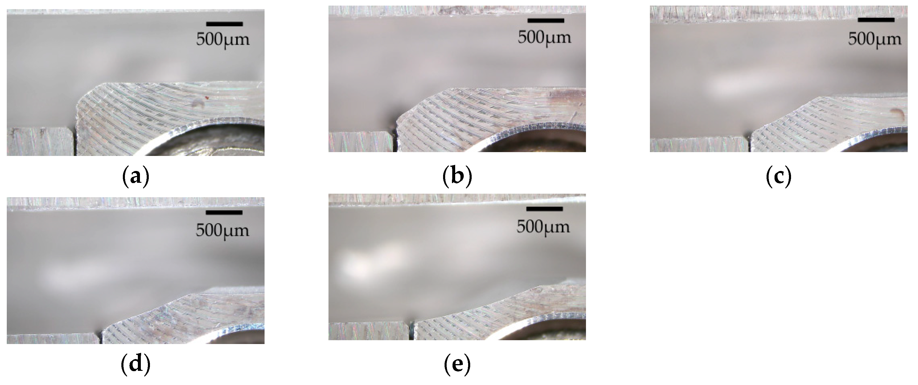
Figure 7 depicts the burr edge erosion at various flow speeds for 200 km of flow length. The effect of flow speed on edge erosion was significant.
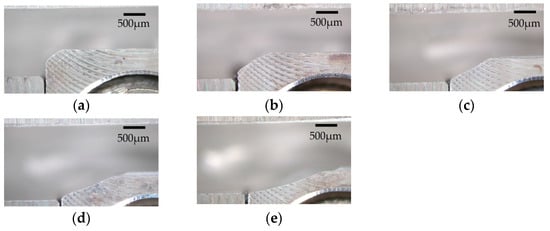
Figure 7.
Progress of burr edge erosion for the flow length of 200 km at various flow speeds, V = (a) 3.3 m/s; (b) 4.5 m/s; (c) 5.6 m/s; (d) 6.7 m/s; (e) 7.8 m/s.
The extent of deburring can be represented by the volume of material removed from the burr edge. Along this line, the reduction in the cross-sectional area of the burr edge can be identified as the deburred area. In Table 2, the observed deburred areas have been listed for different combinations of flow length and flow speed. Figure 8 indicates the graphical representation of Table 2.
Table 2.
Deburred area measured from the preliminary test (in mm2).
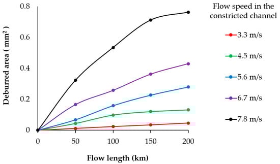
Figure 8.
Deburred area vs. flow length at various flow speeds.
3.4. Chamfering Test and Results
From Figure 7, it can be seen that all the edges were eroded far beyond conventional deburring, except for the flow speed of 3.3 m/s. The right level of flow length was required to be chosen at each flow speed. Figure 9 shows how the flow length levels were estimated for a 45° chamfer off the ideal square edge by 0.2 mm and 0.3 mm. In Figure 9, the gray and yellow dashed lines represent the predicted deburred areas for C0.2 and C0.3. The predicted flow lengths at different flow speeds are listed in Table 3.
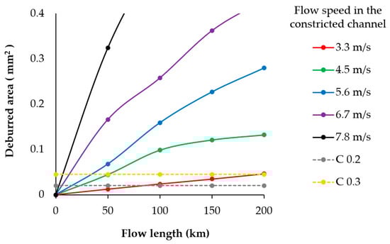
Figure 9.
Deburred area corresponding to C0.2 and C0.3 chamfers.
Table 3.
Predicted flow lengths for C0.2 and C0.3 chamfers at different speeds.
To observe the progress of deburring, the predicted flow lengths for C0.2 were uniformly divided into three steps, and the remaining flow lengths for C0.3 were again divided into three additional steps. For example, for the flow speed of 3.3 m/s, the predicted flow length for C0.2 was 83 km. The predicted six steps of flow lengths for the C0.2 and C0.3 chamfer conditions are listed in Table 4 at each flow speed.
Table 4.
Six steps of flow lengths leading to C0.2 and C0.3 chamfers at various flow speeds.
Figure 10 shows the progress of burr edge erosion in six steps at the flow speed of 7.8 m/s. The chamfered and smoothed edges corresponding to C0.2 and C0.3 are shown in Figure 11.
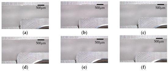
Figure 10.
Progress of burr edge erosion in six steps (Table 4) at the flow speed of 7.8 m/s: (a) 1st step; (b) 2nd step; (c) 3rd step corresponding to C0.2; (d) 4th step; (e) 5th step; (f) 6th step corresponding to C0.3.
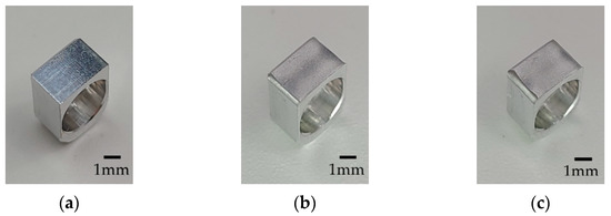
Figure 11.
Deburred edge with C0.2 and C0.3 chamfers at the flow speed of 7.8 m/s: (a) before deburring; (b) C0.2 at step 3; (c) C0.3 at step 6.
Figure 12 shows the deburred edge profiles at the final step for each flow speed. An approximate of C0.3 condition was achieved for all the speeds.
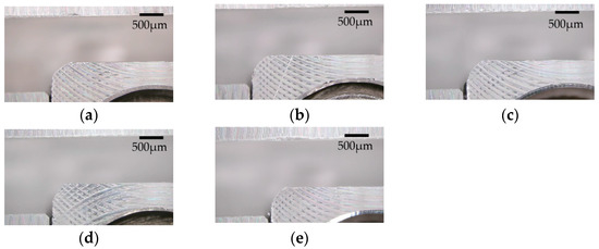
Figure 12.
C0.3 chamfer achieved at the final step six at various flow speeds: (a) 3.3 m/s; (b) 4.5 m/s; (c) 5.6 m/s; (d) 6.7 m/s; (e) 7.8 m/s.
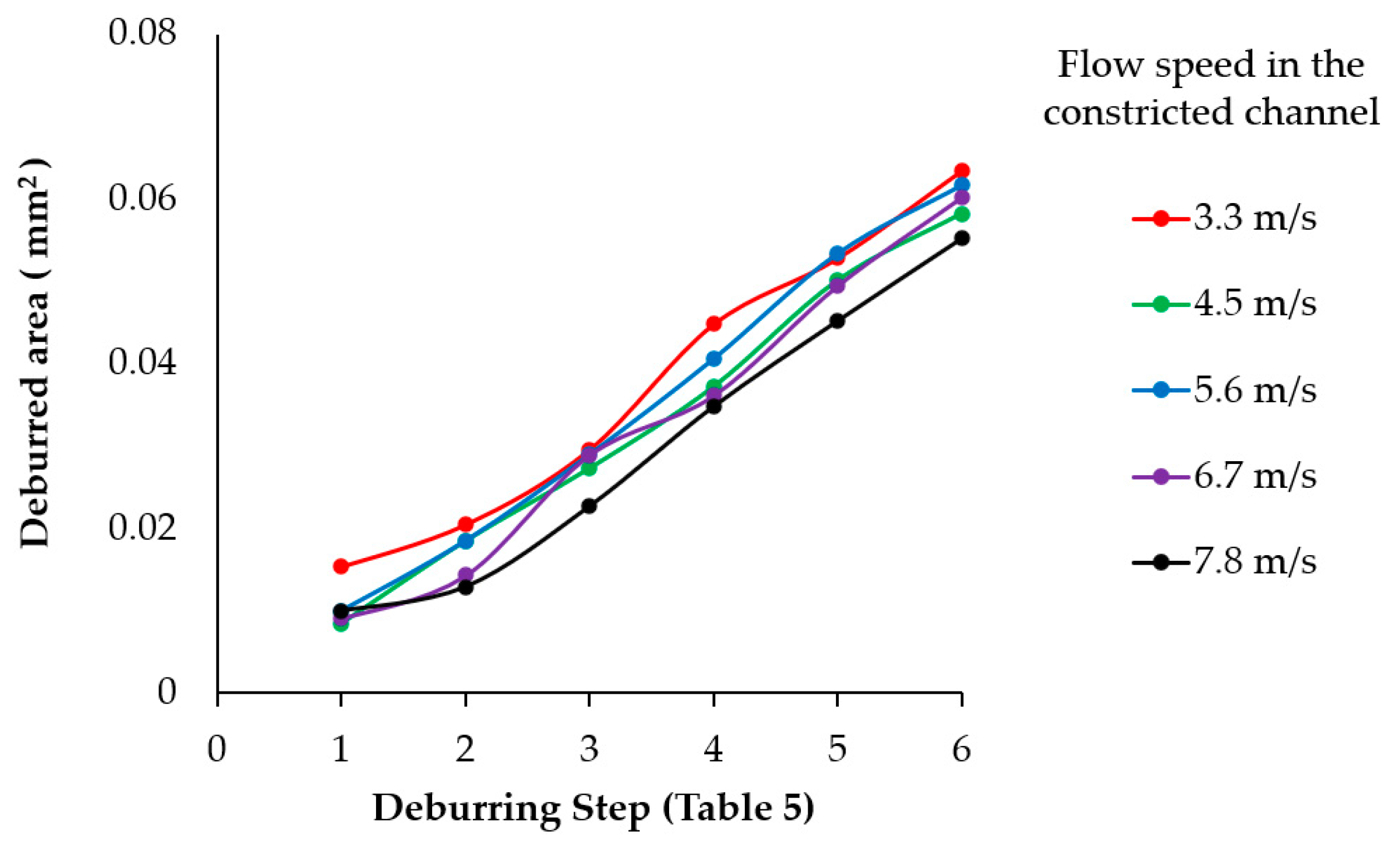
The deburred areas measured for each step at different flow speeds are listed in Table 5. Figure 13 shows a graphical representation of the data in Table 5.
Table 5.
Deburred areas measured for each of the six steps (Table 4) at different flow speeds (in mm2).
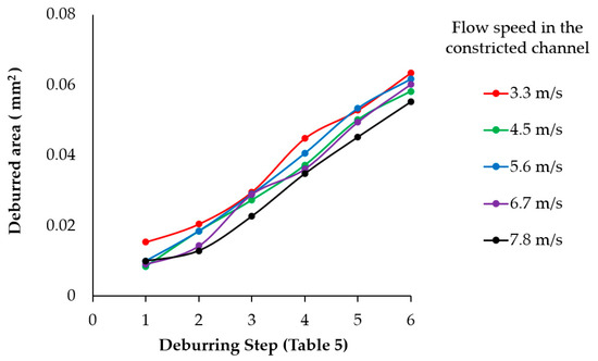
Figure 13.
Deburred area vs. flow length step (Table 4) at different flow speeds.
3.5. Computational Fluid Dynamics (CFD) Model
Local flow conditions near the burr edge, characterized by wall shear stress, streamline geometry, and flow speed, are essential for estimating the objective function. For this purpose, a CFD model was constructed using ANSYS 2019 R1 Fluent. The specimen for the preliminary test was modeled with 706,589 tetrahedral elements and 119,166 nodes, as shown in Figure 14. The element size ranged from 0.25 mm near the burr edge to 5 mm beyond the flow channel. The analysis employed the κ-ω SST model, which offers an advantage when analyzing the wall flow. The viscosity was set to 43.8 poise and the density to 1141 km/m3.
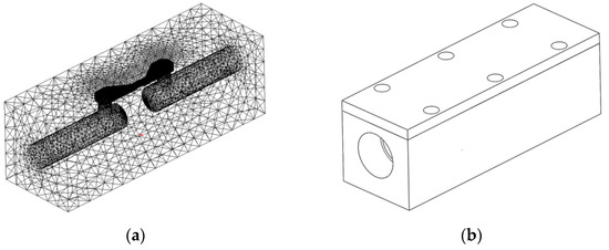
Figure 14.
ANSYS Fluent CFD model for preliminary testing: (a) tetrahedral mesh for the specimen; (b) physical specimen.
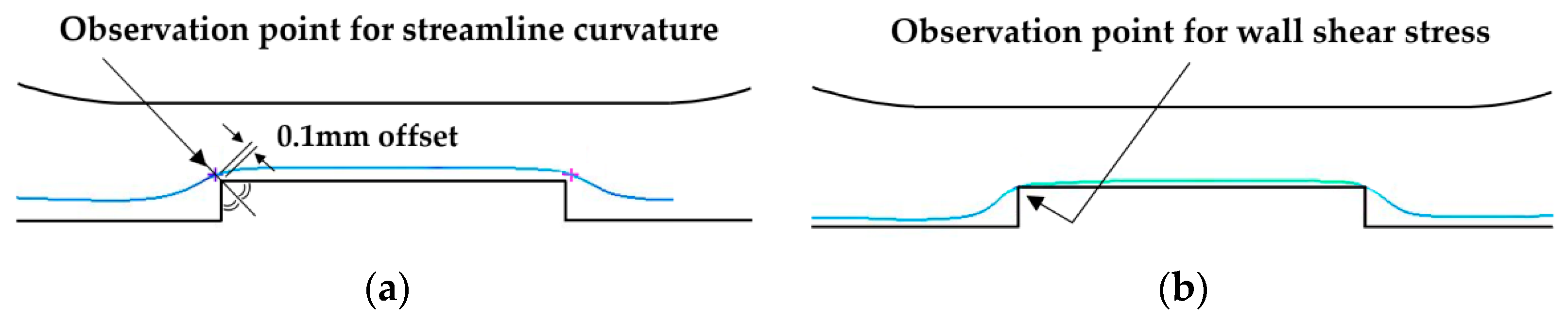
Due to the no-slip boundary condition, streamlines could not be generated at the burr edge. To address this problem, streamlines passing through the 0.1 mm offset position from the burr edge, along the angular bisector, were chosen as shown in Figure 15a. The shear stress was estimated along the burr edge, as shown in Figure 15b.
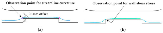
Figure 15.
Observation points for streamline geometry and shear stress in the CFD model: (a) streamline; (b) shear stress.
4. New Objective Function
4.1. Need for a New Objective Function
An ideal objective function represents the actual deburring performance. Table 6 outlines the values of shear stress, local curvature, and Kim’s objective function [18], at each flow speed along with the deburred area for the flow length of 200 km.
Table 6.
Values of objective function suggested by Kim [18] from CFD analyses at different speeds along with the deburred area observed for the flow length of 200 km (Table 2).
When the values of objective function suggested by Kim [18] were compared, they varied from 10.7 N/m to 23.1 N/m when the flow speed increased from 3.3 m/s to 7.8 m/s, respectively. On the other hand, the deburred area for the flow length of 200 km increased from 0.046 mm2 to 0.763 mm2. When the value of the objective function increased 2.2 times, the deburred area increased 16.6 times.
4.2. Suggestion for a New Objective Function
In viscous fluid flow, streamlines cannot be formed along the burr edge due to the no-slip boundary condition. In reality, edge erosion and deburring can be achieved by abrasive flow, which can be understood in terms of pathlines rather than streamlines. A fine abrasive particle can nearly follow a pathline, with random micro-motion generated by the irregularity of the particle geometry. For particles following the pathlines near the burr edge, there are chances for impact and momentum transfer. Meanwhile, pathlines coincide with streamlines for steady flow.
Finnie’s single particle erosion model is defined as follows [23]:
where Q is the volume of material removed, m is the mass of the abrasive particle, Vp is the speed of the abrasive particle, and p is the plastic flow stress of the workpiece. Ψ is the ratio of the depth of collision to the depth of cut. K is the ratio between the vertical and horizontal components of the contact force, and α is the attack angle of particle velocity with respect to the contact surface of the workpiece.
Based on the above equations, the total volume of the eroded material was proportional to the mass of a single particle and the square of the collision speed. A new objective function could thus be proposed along these lines in the following form:
where τxy is the wall shear stress, and κ is the local curvature of the streamline near the burr edge, V is the flow speed at the observation point.
The values of the new objective function at each flow speed, along with Kim’s objective function [18], are listed in Table 7.
Table 7.
Values of Kim’s objective function [18] and the new objective function for different flow speeds.
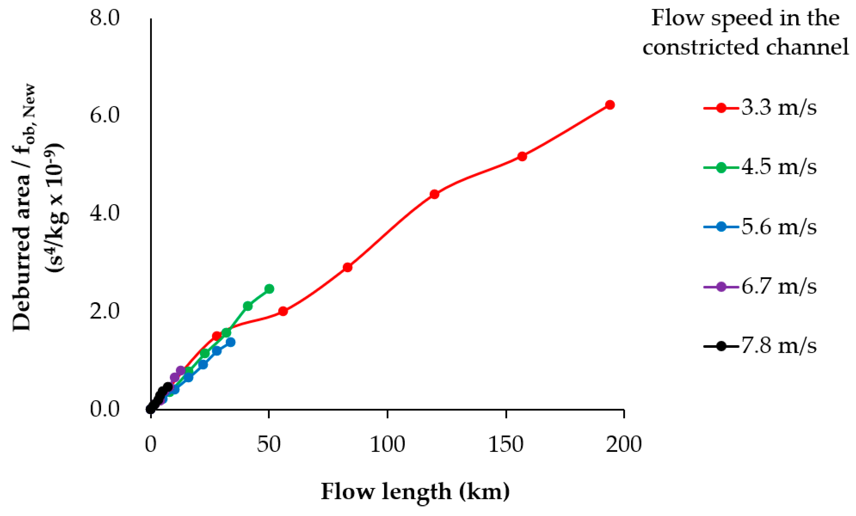
For comparing the new objective function with the one suggested by Kim [18], the values of the deburred area at each of the six steps for various flow speeds in Table 5 were normalized by each of the objective function values enlisted in Table 7, as shown in Figure 16 and Figure 17.
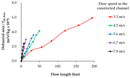
Figure 16.
Deburred area normalized by Kim’s objective function [18] vs. flow length for various flow speeds.
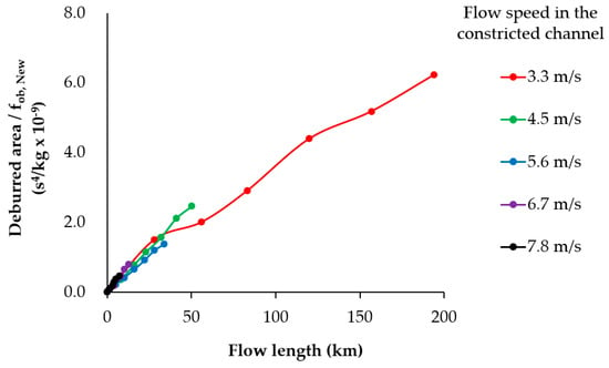
Figure 17.
Deburred area normalized by the new objective function vs. flow length for various flow speeds.
5. Validation of the New Objective Function
5.1. Deburring Test Setup
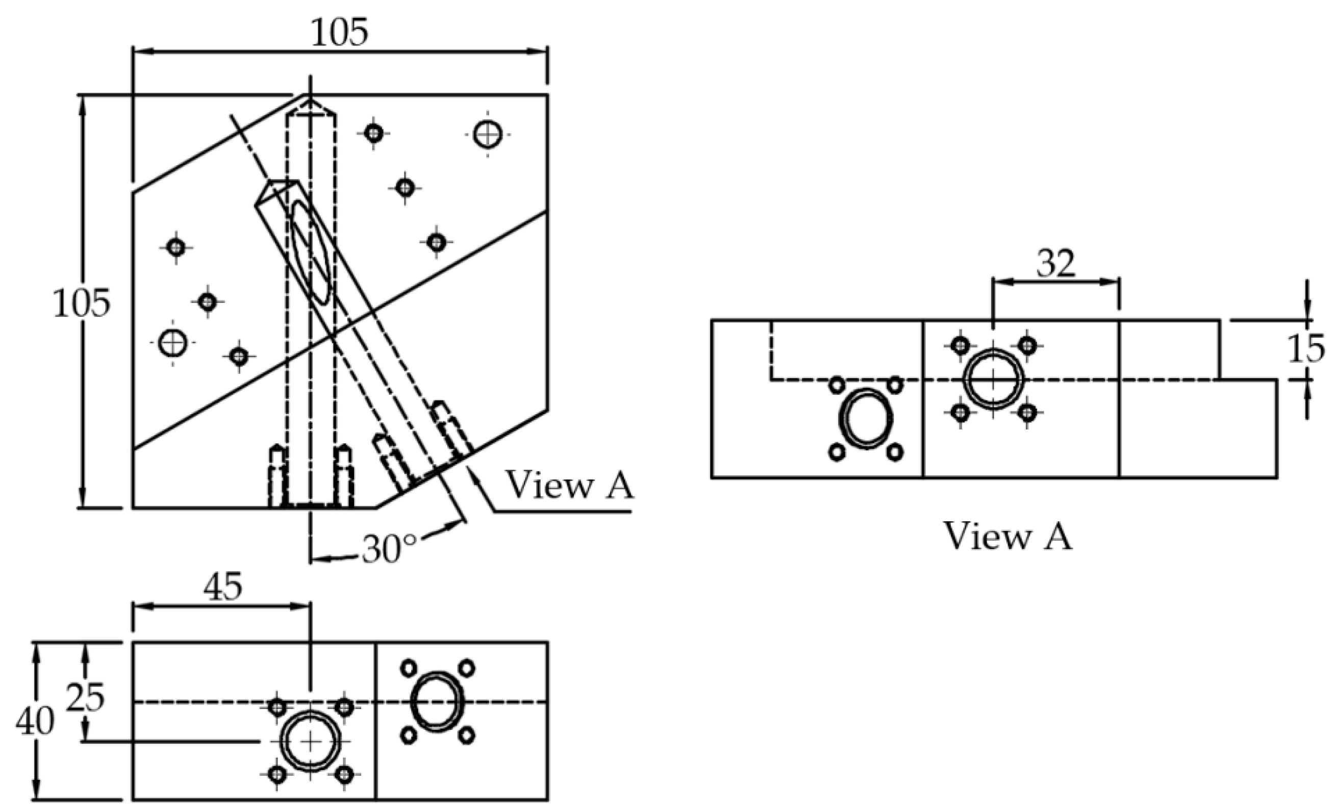
The application of the new objective function for predicting deburring was attempted for two drilled holes of 12 mm diameter, intersecting each other at 30° with 10 mm offset. Figure 18 shows the specimen geometry. The three-dimensional intersection with the varying cross-section along its length posed a challenge for deburring mainly due to poor accessibility. Thinner sections with longer burrs are more difficult to deburr.

Figure 18.
Specimen with a hole intersection (in mm).
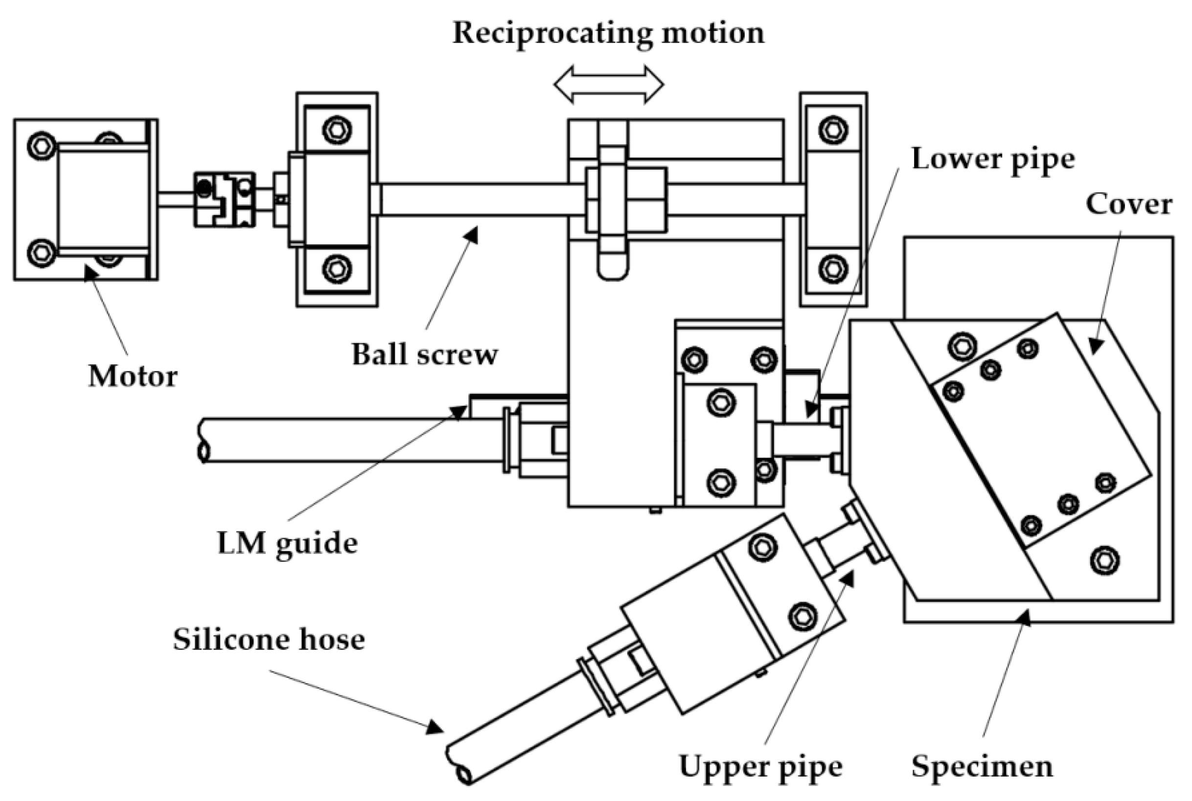
Figure 19 shows the test setup. The specimen body included two intersecting holes. The primary hole was partially sectioned along its length to reveal the intersection. The secondary hole underneath intersected the primary hole. Each of the holes was connected to the pipes and hoses. The upper pipe for the primary hole accommodated an insert to constrict and intensify flow to the narrow annulus along the burr edge. The lower pipe had a slotted opening to further constrict the flow locally. The lower pipe was allowed to reciprocate along its axis for uniform deburring along the length of the intersection.

Figure 19.
Test setup for deburring.
The upper pipe connected to a silicone hose was fixed with respect to the specimen. The lower pipe, also connected to a silicone hose, was driven by a linear actuator system, including a ball screw, linear motion guide, drive motor, and control circuitry.
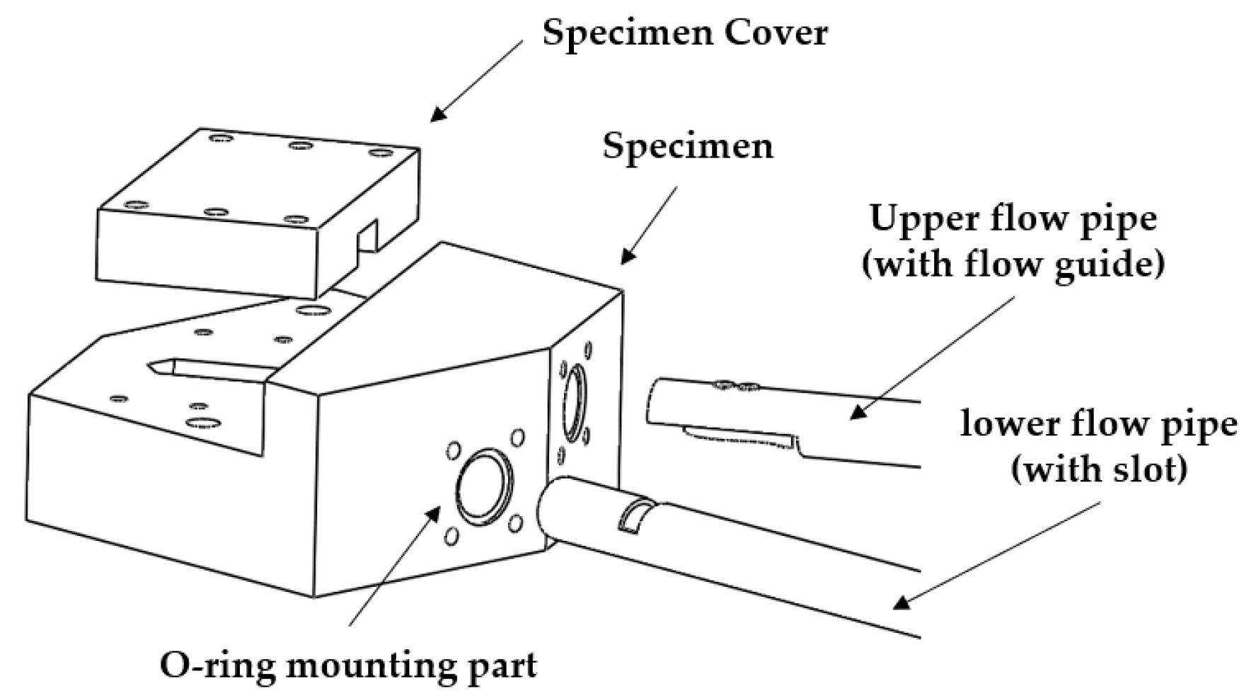
Figure 20 indicates the details of the specimen with the upper and lower pipes, cover, and O-ring for sealing. The lower pipe was continuously reciprocated by a NEMA 17 stepping motor. Deburring progress could be observed by opening the cover.
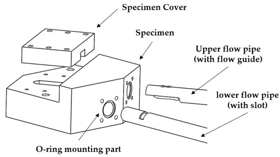
Figure 20.
Specimen, upper flow pipe with the flow guide, and the lower flow pipe with a slot.
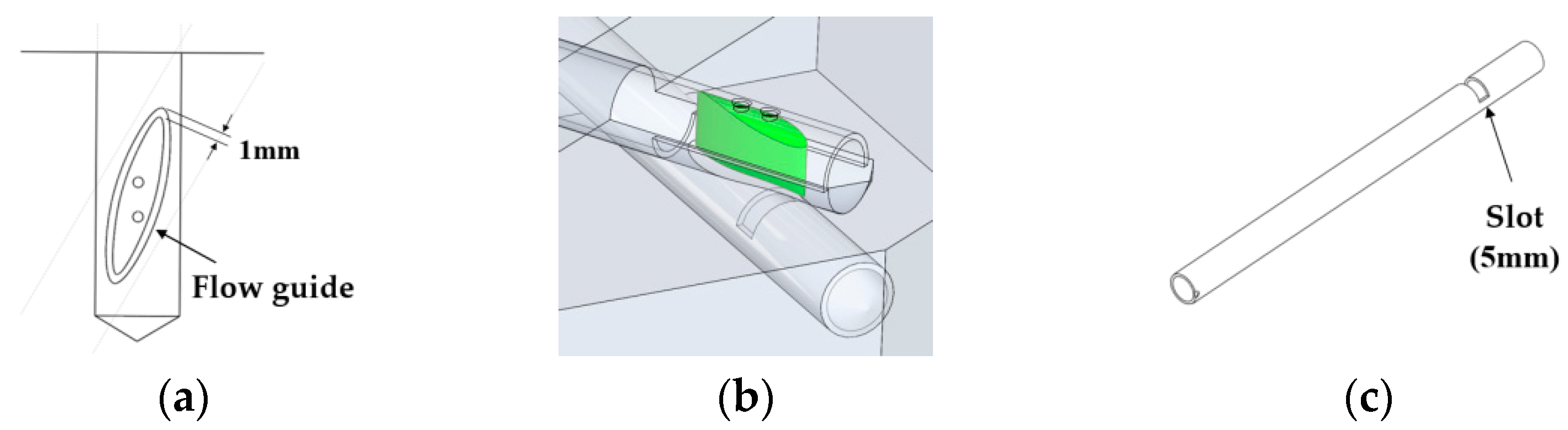
As shown in Figure 21a, the flow guide was designed to confine the flow within an annulus zone of 1 mm width between its lower end and the intersection. The lower pipe had a slot of 5 mm width. By combining the flow guide and the slot, the abrasive flow began from the upper pipe, proceeded to the annulus, then the slot, and finally the lower pipe when the flow began from the upper pipe. The flow conditions were reversed when the abrasive flow began from the lower pipe.

Figure 21.
Flow passage through the intersection: (a) annulus between the lower end of the flow guide and intersection; (b) assembly of the upper flow pipe and flow guide; (c) slotted opening of 5 mm width in the lower flow pipe.
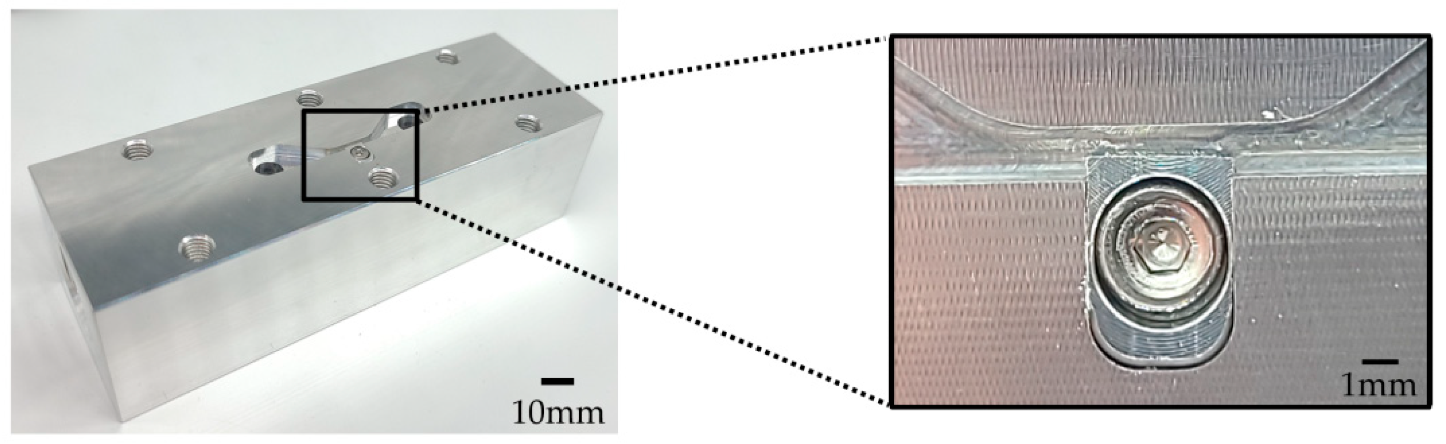
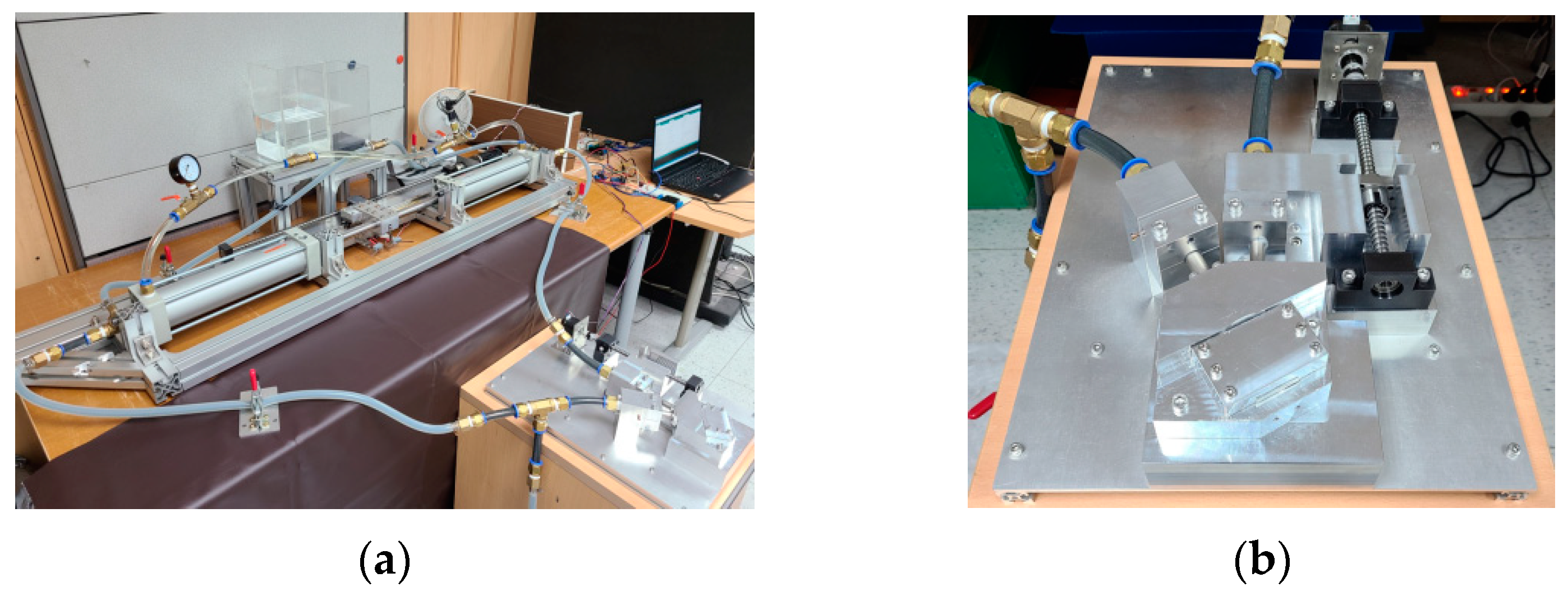
Figure 22 shows the photographs of the test setup and specimen for the validation test.
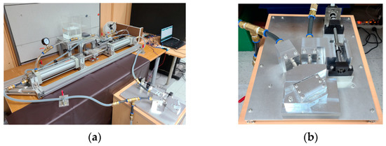
Figure 22.
Photographs of (a) test setup; (b) a close-up view of the specimen.
5.2. Deburring Test Results
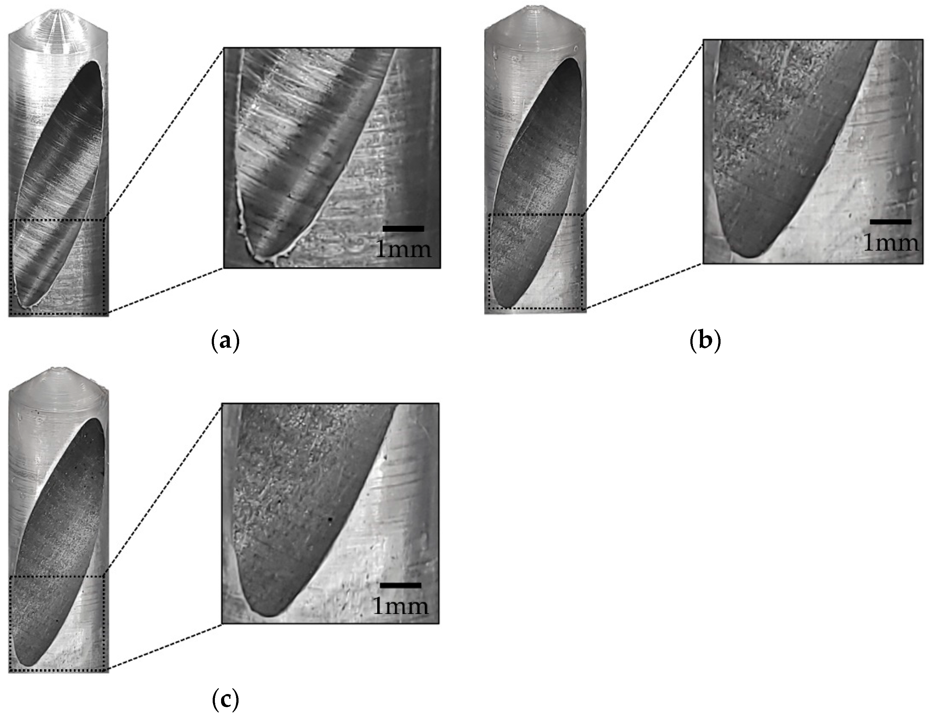
The inlet flow speed for the pipes was fixed at 1 m/s. In this test, the flow length was defined with respect to the inlet flow. The viscosity of the abrasive fluid and grit number of the abrasive particles was the same as before, 43.8 poise and #100, respectively. The test was carried out up to the flow length of 112 km. The test results are shown in Figure 23.
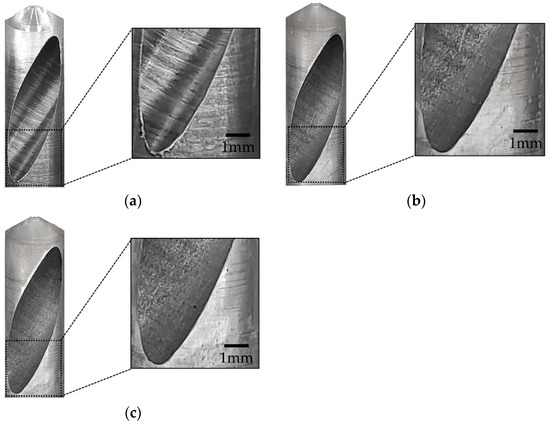
Figure 23.
Results of the deburring test: (a) before deburring; (b) 56 km run; (c) 112 km run.
Before deburring, large burrs were observed particularly at the thinner sections of the intersection. At the flow length of 56 km, these large burrs were removed with minor residues. At 112 km, edge rounding was observed after the complete removal of burrs.
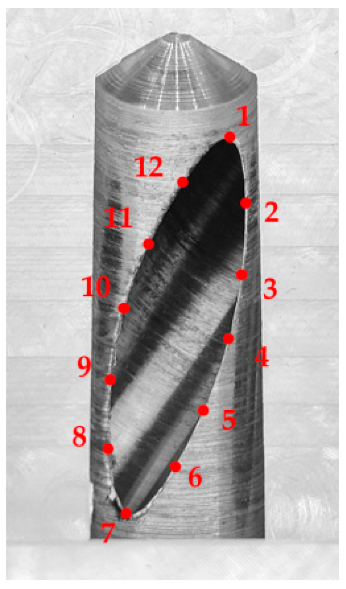
To further examine the progress of deburring with respect to the edge cross section, 12 positions along the burr edge were defined as shown in Figure 24. The uppermost position with the thinnest cross-section hole was defined as position 1. The remaining 11 positions were sequentially defined clockwise from position 1, at equal distances along the edge.
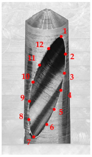
Figure 24.
Twelve positions on the burr edge for cross-sectional examination.
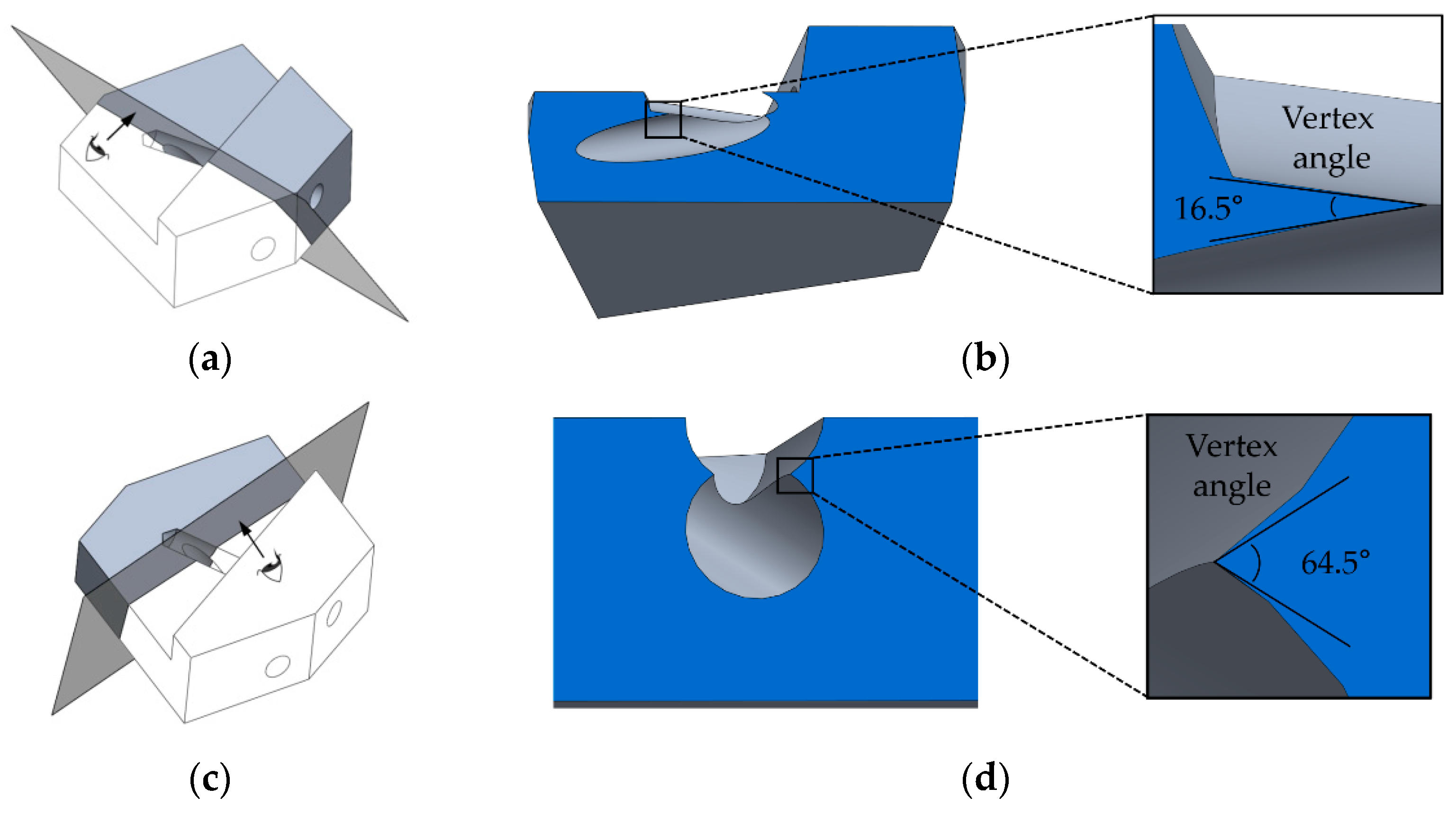
Figure 25 shows the cross sections for positions 1 and 4. The sections were thinnest at position 1 and thickest at position 4. These cross sections were generated perpendicular to the intersection at each position.
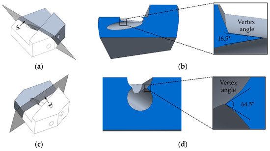
Figure 25.
(a) Cross sections of the specimen along the intersection: (a) cross section at position 1; (b) close-up view of the cross section at position 1; (c) cross section at position 4; (d) close-up view of the cross section at position 4.
The cross-sectional vertex angles at each of the twelve positions along the intersection are listed in Table 8.
Table 8.
Cross-sectional vertex angles at the 12 positions along the intersection (Figure 24).
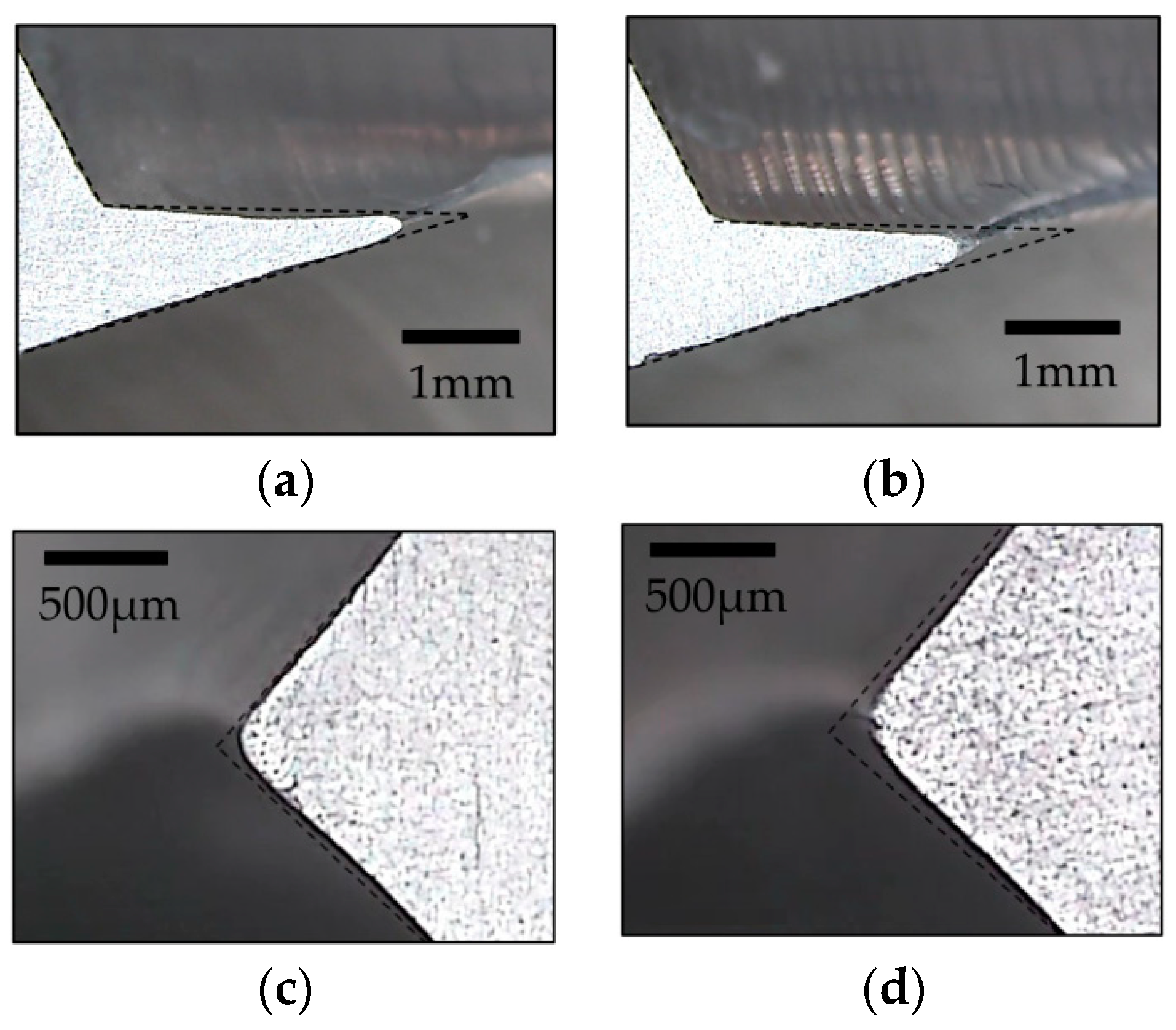
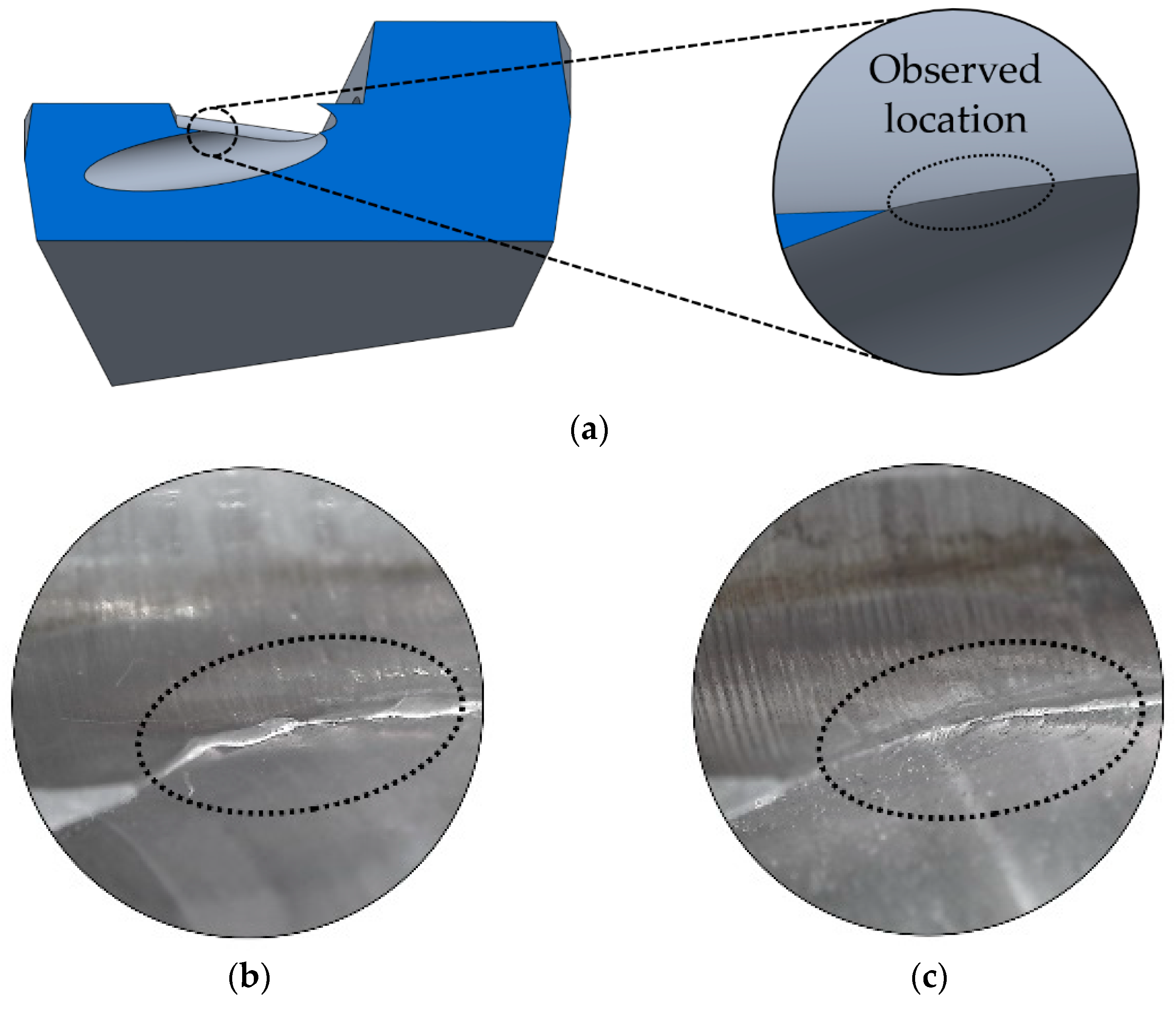
Figure 26 shows the photographs of the edge cross sections at positions 1 and 4 for the 56 km and 112 km flow lengths, respectively. The dotted lines represent the ideal sectional profile without burrs before deburring. The deburred areas measured for each position at different flow lengths are listed in Table 9.
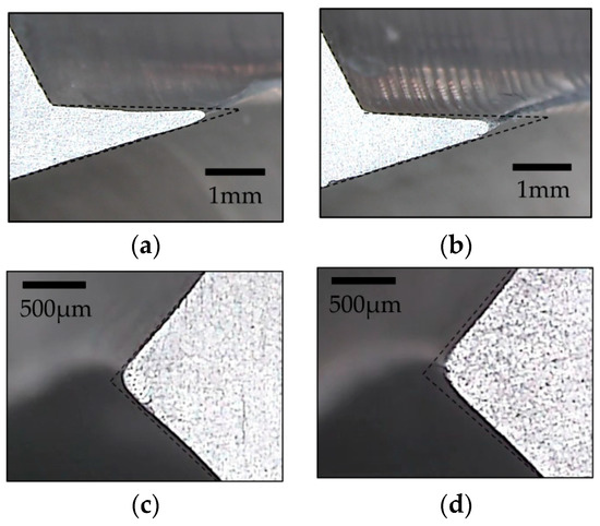
Figure 26.
Sectional profiles after deburring at positions 1 and 4: (a) position 1, flow length of 56 km; (b) position 1, flow length of 112 km; (c) position 4, flow length of 56 km; (d) position 4, flow length of 112 km.
Table 9.
Deburred areas measured from the validation test (in mm2).
Figure 26 indicates the complete removal of burrs at positions 1 and 4 for the flow length of 56 km. However, this can be somewhat misleading because residual burrs can also be observed in the vicinity between positions 1 and 2, as shown in Figure 27. The irregular and rough edges in Figure 27b, for the flow length of 56 km, could be owing to the random failure of large burrs and subsequent erosion of the remaining roots. For the flow length of 112 km, Figure 27c shows significantly reduced irregularity and roughness.

Figure 27.
Burr edge between positions 1 and 2 (Figure 24): (a) edge location; (b) after the flow length of 56 km; (c) after the flow length of 112 km.
5.3. CFD Model
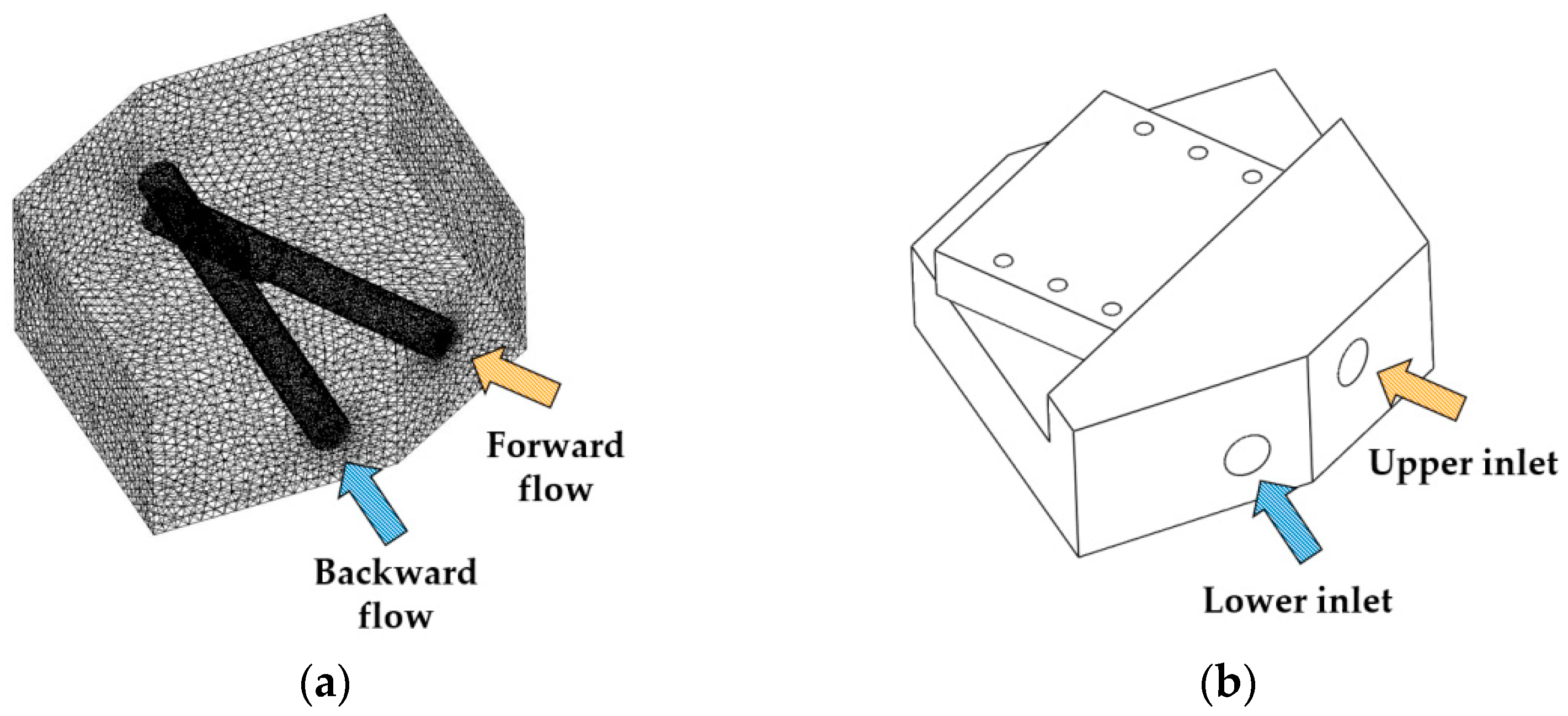
CFD simulations were performed by using ANSYS 2019 R1 Fluent to calculate the objective function values for validation. The specimen modeled with 1.32 million tetrahedral elements and 230,000 nodes is shown in Figure 28. The element size ranged from 0.5 mm near the burr edge to 3 mm beyond the fluid passage. The simulations were performed for the forward flow from the upper pipe and the backward flow from the lower pipe.
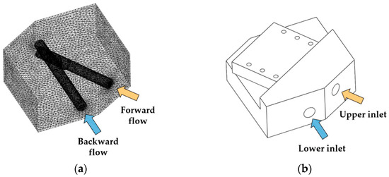
Figure 28.
ANSYS Fluent CFD model for deburring at the intersection between the offset holes: (a) tetrahedral mesh for the specimen; (b) physical specimen.
5.4. CFD Simulation and Validation of the New Objective Function
From the CFD simulations, the shear stress and streamline curvature were obtained in the cross sections for each of the 12 positions. It was assumed that the flow component in the tangential direction to the intersection had little contribution to the deburring. Thus, the values of the new objective function were calculated in terms of the cross-sectional values. As in the case of preliminary test simulations, the observation point definition of 0.1 mm offset from the vertex along the angular bisector was adopted.
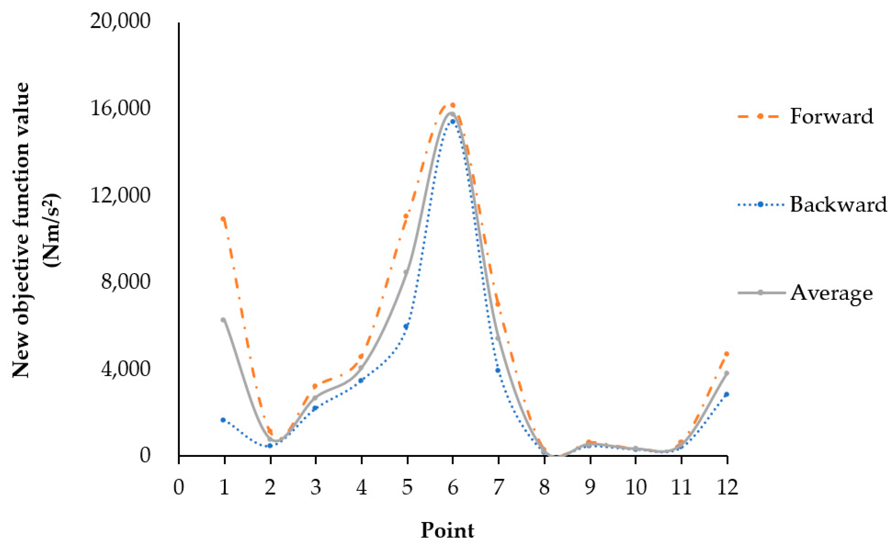
The new objective function values at the 12 positions for the forward and backward flows are listed in Table 10. Figure 29 is a graphical representation of Table 10.
Table 10.
New objective function values at 12 positions (Figure 24) for the forward and backward flows.
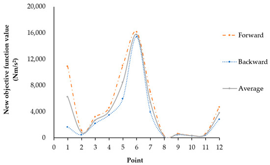
Figure 29.
New objective function value vs. position on the burr edge (Figure 24).
As shown in Table 11, the ratio of the average values for position 1 to position 4 is 1.55 for the new objective function while it is 0.41 for the previous objective function suggested by Kim et al. [18]. The ratio of the deburred areas from position 1 to the position for flow lengths of 56 km and 112 km are 1.50 and 1.58, respectively. The new objective function based on CFD simulation seems to represent the deburring performance with reasonable accuracy.
Table 11.
Average values of the objective functions and the sectional deburred area measured at positions 1 and 4 for flow lengths of 56 km and 112 km.
6. Conclusions
In this study, deburring was conducted by AFM with a low-viscosity abrasive medium at high-flow speeds. Kim [18] previously suggested that deburring performance is affected by the local curvature of the streamline near the burr edge and wall shear stress. It was expected that flow speed would also have a significant effect, and Kim’s objective function was supplemented with V2, representing the kinetic energy of the abrasive particles near the burr edge. To observe and verify this concept, preliminary deburring tests were performed on a set of milling workpieces along with CFD simulations for planar flow. The experiments were performed in six stages, and deburring progress was observed. The progress was characterized by the volume of material removed from the ideal burr edge. It was confirmed that the progress soundly correlates with the new objective function value, as shown in Figure 16 and Figure 17.
Under the assumption that the flow component is tangential to the burr edge has relatively little contribution to the deburring, the new objective function has a potential for general applications beyond the planar flow. Along this line, the application of the new objective function to the erosion of the burr edge is formed by two drilled holes of 12 mm diameter, intersecting at 30° with a 10 mm offset. Such configuration generates very thin burr edges that are most favorable to burr formation. For observations, two positions (1 and 4) along the burr edge were selected, representing the thinnest and thickest sections. From the CFD simulations, the ratio of the new objective function values at positions 1 and 4 was 1.55, as listed in Table 11. From the experiments, the ratios of the actual deburred area for the first and the second stages of deburring each, up to 56 km and 112 km of flow lengths, were 1.50 and 1.58, respectively. The new objective function thus seems to have a potential, with reasonable accuracy, for industrial applications for predictions and optimizations of deburring processes based on CFD simulations.
Author Contributions
Conceptualization, K.-J.K. and K.-H.K.; methodology, K.-J.K. and Y.-G.K.; validation, K.-J.K.; formal analysis, K.-J.K. and K.-H.K.; investigation, K.-J.K. and Y.-G.K.; data curation, K.-J.K.; writing—original draft preparation, K.-J.K.; writing—review and editing, All; visualization, K.-J.K.; supervision, K.-H.K. All authors have read and agreed to the published version of the manuscript.
Funding
This research received no external funding.
Institutional Review Board Statement
Not applicable.
Informed Consent Statement
Not applicable.
Data Availability Statement
The data generated in this study are freely available.
Conflicts of Interest
The authors declare no conflict of interest.
References
- Gillespie, L.K. Deburring precision miniature parts. Precis. Eng. 1979, 1, 189–198. [Google Scholar] [CrossRef]
- Saptaji, K.; Triawan, F.; Sai, T.; Gebremariam, A. Deburring method of aluminum mold produced by milling process for microfluidic device fabrication. Indones. J. Sci. Technol. 2021, 6, 123–140. [Google Scholar] [CrossRef]
- Cho, C.H.; Kim, J.H.; Chae, S.W.; Kim, K.H. Improvement of a deburring tool for intersecting holes with reduced irregular cutting of burr edge. J. Eng. Manuf. 2013, 227, 1693–1703. [Google Scholar] [CrossRef]
- Kadam, S.P.; Mitra, S. Electrochemical deburring—A comprehensive review. Mater. Today Proc. 2021, 46, 141–148. [Google Scholar] [CrossRef]
- Kumar, A.S.; Deb, S.; Paul, S. Ultrasonic assisted abrasive micro-deburring of micromachined metallic alloys. J. Manuf. Process. 2021, 66, 595–607. [Google Scholar] [CrossRef]
- Balasubramaniam, R.; Krishnan, J.; Ramakrishnan, N. An experimental study on the abrasive jet deburring of cross-drilled holes. J. Mater. Process. Technol. 1999, 91, 178–182. [Google Scholar] [CrossRef]
- Jakub, M. Effect of ceramic brush treatment on the surface quality and edge condition of aluminum alloy after abrasive waterjet machining. Adv. Sci. Technol. Res. J. 2021, 15, 254–263. [Google Scholar]
- Yu, I.K. Improvement of the technological process of processing parts of coaxial radio components using thermal impulse deburring. J. Phys. Conf. Ser. 2021, 2032, 012066. [Google Scholar]
- Kwon, B.C.; Kim, K.H.; Kim, K.H.; Ko, S.L. New abrasive deburring method using suction for micro burrs at intersecting holes. CIRP Ann. 2016, 65, 145–148. [Google Scholar] [CrossRef]
- Sehijpal, S.; Shan, H.S. Development of magneto abrasive flow machining process. Int. J. Mach. Tools Manuf. 2002, 42, 953–959. [Google Scholar]
- Larry, R. Abrasive flow machining: A case study. J. Mater. Process. Technol. 1991, 28, 107–116. [Google Scholar]
- Dixit, N.; Sharma, V.; Kumar, P. Research trends in abrasive flow machining: A systematic review. J. Manuf. Process. 2021, 64, 1434–1461. [Google Scholar] [CrossRef]
- Kum, C.W.; Wu, C.H.; Wan, S.; Kang, C.W. Prediction and compensation of material removal for abrasive flow machining of additively manufactured metal components. J. Mater. Process. Technol. 2020, 282, 116704. [Google Scholar] [CrossRef]
- Choi, J.Y.; Kim, K.H. Research on the Deburring of Burr Edge at the Intersection of Small Holes. Master’s Thesis, Korea University, Seoul, Korea, 2015. [Google Scholar]
- Beom, J.K.; Kim, Y.G.; Kim, K.H. Study on the Deburring of Intersecting Holes with Abrasive Flow Machining. Master’s Thesis, Korea University, Seoul, Korea, 2018. [Google Scholar]
- Kim, K.J.; Kim, Y.G.; Kim, K.H. Deburring. Deburring of offset hole intersection with abrasive flow machining. Trans. Korean Soc. Mech. Eng. 2019, 43, 507–511. [Google Scholar] [CrossRef]
- Kim, D.W.; Kim, K.H. Removal of Drilling-Milling Composite Burrs by Abrasive Flow. Master’s Thesis, Korea University, Seoul, Korea, 2018. [Google Scholar]
- Kim, Y.G.; Kim, K.J.; Kim, K.H. Efficient Removal of milling Burrs by abrasive flow. Int. J. Precis. Eng. Manuf. 2021, 22, 441–451. [Google Scholar] [CrossRef]
- Uhlmann, E.; Mihotovic, V.; Szulczynski, H.; Kretzschmar, M. Developing a Process Model for Abrasive Flow Machining. In Burrs—Analysis, Control and Removal; Springer: Berlin/Heidelberg, Germany, 2010; pp. 73–78. [Google Scholar]
- Chen, X.; McLaury, B.S.; Shirazi, S.A. Numerical and experimental investigation of the relative erosion severity between plugged tees and elbows in dilute gas/solid two-phase flow. Wear 2006, 261, 715–729. [Google Scholar] [CrossRef]
- Edwards, J.K.; McLaury, B.S.; Shirazi, S.A. Modeling solid particle erosion in elbows and plugged tees. J. Energy Resour. Technol. 2001, 123, 277–284. [Google Scholar] [CrossRef]
- Wong, C.Y.; Solnordal, C.; Swallow, A.; Wu, J. Experimental and computational modelling of slid particle erosion in a pipe annular cavity. Wear 2013, 303, 109–129. [Google Scholar] [CrossRef]
- Finnie, I. Erosion of surfaces by solid particles. Wear 1960, 3, 87–103. [Google Scholar] [CrossRef]


Publisher’s Note: MDPI stays neutral with regard to jurisdictional claims in published maps and institutional affiliations. |
© 2022 by the authors. Licensee MDPI, Basel, Switzerland. This article is an open access article distributed under the terms and conditions of the Creative Commons Attribution (CC BY) license (https://creativecommons.org/licenses/by/4.0/).