1. Introduction
A typical aspect of the observed seismicity in the northern and central Apennines, and in the whole Italian region more generally, is the occurrence of earthquake sequences characterized by multiple, similarly large mainshocks. An example of this behavior is the quantitative model “Every Earthquake Precursory According to Scale” (EEPAS), applied by Rhoades and Evison [
1,
2,
3]. According to their quantitative definition, introduced by Evison and Rhoades [
4], swarms are seismic sequences constituted by at least three earthquakes whose magnitudes are linked to each other by empirical rules.
In this study we define as a multiplet a set of two or more earthquakes, with the following conditions: (a) the first event has a magnitude equal to or larger than a given threshold; (b) the others occur within a time difference and distance defined by the Gardner and Knopoff [
5] criterion from each other; and (c) within a given magnitude range. This definition is different from that usually applied for common seismicity patterns such as foreshock–aftershock sequences and clusters (e.g., Gentili and Di Giovambattista [
6]).
Building upon a previous paper (Console et al. [
7]), in which we examined the aspect of multiple mainshocks in central Italy, in this study we aim at verifying if a synthetic catalog reproduces this kind of earthquake clustering. For this purpose, we apply a new version of the simulator algorithm, in which the role of stress transfer among elements of an expanding rupture is enhanced. Moreover, we give also examples of other space-time seismic features exhibited by synthetic catalogs, both in short- (days–months) and long-term (years–centuries), some of which were observed in real earthquake catalogs.
In
Section 2 we present a brief description of the algorithm used for detecting multiple events in an earthquake catalog, based on the previously cited (a), (b), and (c) criteria. This algorithm is applied for providing a possible metric for comparing real observations with simulations.
Section 3 gives an outline of the seismotectonic model of our study area of northern and central Apennines, along with examples of recent and historical sequences of multiple mainshocks observed in this region.
In
Section 4, after a short introduction of the new version of the simulator employed in this study, we show the results obtained applying this simulation code to the above mentioned seismotectonic model of the study area. Having tried three choices for the two main free parameters present in the algorithm, for a total of nine different combinations, we chose one of them by a criterion based on the analysis of the multiplets in the synthetic catalog of 100,000 years. Some features of this preferred simulated catalog are then compared in several ways with a real set of observations lasting only 370 years in the same seismogenic area.
Section 5 reports other results of spatio-temporal analysis of the same 100,000 years simulated catalog that appear to be consistent in reasonable way with real seismicity patterns not strictly related to our study area. In particular, we show that the use of simulators allows testing hypotheses of seismogenic models in a way that is not possible on the basis of real observations, due to lack of completeness and homogeneity of these observations in the long-term.
2. The Algorithm for Identification of Multiple Events
A special algorithm for the search of multiple events in a seismic catalog was created to use it as metrics in the comparison between the simulator results and the observed seismicity of the studied region. The computer code is “customer-built” and it was already introduced by Console et al. [
7]. There is no specific definition of “sequence with multiple main shocks”, nor any fixed magnitude values. We give here a brief description for a better understanding of its use. At its first level, the algorithm systematically analyzes time-ordered couples of events to check if they meet some constitutive conditions. Once matching couples are found, they are then used as elements for ordered noncyclic graph construction. These graphs can be ‘traversed’ to find in them the searched multiple events groups. In accordance with the above definitions, we developed a method based on four criteria for our comparisons among couples of events (
Table 1):
There is a minimum magnitude threshold for the first event of the group (hereafter called “pivot”);
The magnitude of any other main shocks of the sequence must lay in a predefined neighborhood of the pivot’s magnitude;
The events’ time differences must be less than a threshold time, which is a function of event magnitudes (subject to criteria #1 and #2);
For any event, a magnitude dependent distance (a radius) is defined and the distance between the epicentres must be smaller than a proper function of those radii.
The values associated to the criteria #1 and #2 are selected by the user and based on needs, expert judgment and/or knowledge of the instrumental–historical seismicity of the area. The relations for time (#3) and distance (#4) thresholds as a function of event magnitudes were derived from Gardner and Knopoff [
5] empiric tables and as epicentre distance threshold. Notice that the criterion #3 does not provide for a choice, while the criterion #4 provides for the choice among three different ways of applying the formulas of Gardner and Knopoff [
5]. In this study, we used the sum of the radii. Once launched, the algorithm parses the catalog through a cyclic, the three-step analysis procedure is repeated until the end of the file:
The first step starts with the selection of the next pivot event and the definition of a pool of eligible events (if they exist). They are found using criterion #3;
The second phase is a thorough analysis of all useful couples taken from the pool, checked for fulfillment of criteria #1, #2 and #4;
The last step is the construction of the graph, its traversal for the multiplets group search, its eventual output in the output buffer, and the flagging of used events to not reuse them after the next pivot search.
Table 1 summarizes the formulas, explaining the rationale by which they were used in this study, and lists our choices for the threshold values.
Even if the algorithm cannot be called “optimal” in principle, since it is based on an arbitrary choice among possible criteria, it is, however, quite effective, and its importance lays in the metrics it represents for comparison among seismic catalogs.
3. Seismotectonic Model
The seismogenic model of the study area straddles northern and central Italy from the large flat area of the Po Plain (to the north) toward the northern flank of the Gran Sasso mountain range, the highest sector of the Apennines (to the south,
Figure 1). The study area is wider than that previously studied (Console et al. [
8]) through an old version of the simulator and the seismogenic sources now come from the latest 3.3.0 version of the DISS (DISS Working Group [
9]).
Historical and instrumental seismicity in the study area is mainly distributed along the axis of the northern and central Apennines chain and, secondarily, in correspondence with its foothills, plains, and coastal areas (Rovida et al. [
10]). The causative sources of the earthquakes of these two regions have different parameters and kinematics, as shown by focal mechanisms (Pondrelli et al. [
11]), active stress indicators (Mariucci and Montone [
12]), geological data (see DISS Working Group [
9] and references therein), and active strain data (Devoti et al. [
13]). As matter of fact, the GPS data show the crustal extension at a rate of about 3 mm/yr across the Apennines belt and the compression towards the Adriatic foreland (Devoti et al. [
13]).
The active extension along the backbone of the Apennines is accommodated by normal faulting, which dominates along the hinge of the chain at shallow crustal seismogenic depth (blue polygons in
Figure 1; e.g., Vannoli et al. [
14]). The strongest extensional recent earthquakes in the study area occurred during the 2016–2017 central Italy seismic sequence that struck central Apennines with multiple mainshocks (
Table 2). The sequence initiated on 24 August 2016 with the
Amatrice earthquake and was followed on 26 October 2016 by the
Visso earthquake, about 25 km to the north. The largest event, the
Norcia earthquake, occurred on 30 October 2016 and nucleated between the source regions of the two previous mainshocks (e.g., Michele et al. [
15]; Rovida et al. [
10]). Low-magnitude earthquakes of this sequence still occur today (
http://terremoti.ingv.it/ accessed on 22 November 2021). This seismic sequence activated a circa 80 km long, NNW-SSE trending, low-angle multiple fault systems (IDs 127 and 128 in
Figure 1). These fault systems exhibit complex ruptures and are the easternmost normal faults of the central Apennines, just west of where compressional activity prevails (e.g., Basili et al. [
16]; Bonini et al. [
17]; Di Bucci et al. [
18]; DISS Working Group [
9]).
The active compression in the Adriatic foreland is mainly accommodated by thrust faulting (e.g., Vannoli et al. [
19], Vannoli et al. [
20]). Thrust faulting is widespread along the external fronts (red polygons in
Figure 1) and propagates from the inner and coastal areas towards the offshore (to the east) and the Po Plain (to the north). Strongest recent compressional earthquakes of the study area occurred in Emilia during the 2012 sequence. This sequence began with the 20 May
earthquake and was followed on 29 May 2012 by the
earthquake; therefore, it is characterized by two similarly large mainshocks (see also
Figure 1 in Console et al. [
7]). The causative faults systems of the 2012 sequence are the external arcs of the most advanced and buried portions of the northern Apennines (IDs 103 and 51 in
Figure 1; e.g., Vannoli et al. [
20]).
Therefore, the seismogenic model of northern and central Apennines includes onshore and offshore seismogenic sources characterized by both extensional and compressive kinematics (DISS Working Group [
9]). In addition, dextral strike-slip faulting is present in the southernmost study area, at the northern border of the Gran Sasso ridge (green polygons in
Figure 1). Generally, the transverse structures are faults inherited from older tectonic phases that cut the Adriatic foreland areas accommodating the segmentation of the thrust fronts and the outward propagation of the fold and thrust belts (e.g., Zampieri et al. [
21]). Specifically, these strike-slip sources are high-angle, ENE–WSW-trending faults bounding the central Apennines thrust fronts and the southern part of the Apennines basal decollement. They are relatively deep (having 15–20 km of maximum depth), with shear zones that affect the Adriatic foreland (IDs 135 and 134). The western source (ID 135) is believed to be responsible for the seismic sequence that includes two relatively similar large mainshocks that occurred on 5 September 1950 (
) and 8 August 1951 (
; see
Table 2).
In summary, the earthquake sequences characterized by at least two similarly large mainshocks are rather common in the study area, affect compressional, extensional, and strike-slip environments, and are very different from the sequences made up of a single large earthquake followed by aftershocks of decreasing magnitude.
Figure 2 shows the epicentres of the CPTI15 catalog from 1650 to 2020, with
, and the colored lines connect the multiple main shocks events recognized by the algorithm described in the text and reported in column “Csum” of the
Table 2. In the same Table the column “C1st” shows the results of the algorithm applying the criterion 4a.
The seismogenic model upon which we applied the simulator code was derived from the Composite Seismogenic Sources (CSS) of DISS, version 3.3.0 (DISS Working Group [
9]). The CSSs are parameterized crustal faults based on regional surface and subsurface geological data, and they are believed to be capable of producing
earthquakes. We converted the 43 CSSs identified in the study area into 198 quadrilaterals specifically developed for this study, and this is consistent with all the geometrical and kinematics parameters supplied for the CSSs (
Figure 1). The
Table S1 in the Supplementary Material reports the list and the parameters of the 198 quadrilaterals recognized in the study area.
Figure S4 shows a sketch of a quadrilateral fault segment and the description of its geometrical parameters.
4. Simulation of the Seismicity
By means of a newly developed version of our physically based simulation code Console et al. [
22] and references therein), we compiled synthetic earthquake catalogs lasting 100,000 years for events of magnitude
within the polygonal area depicted in
Figure 1. In this version, no application is performed on the State and Rate formulation, but we adopted an enhanced role of the static Coulomb stress transfer between every ruptured element of the fault model and all the other elements in the surrounding faults. In this new version of the code, the magnitude distribution of the simulated catalog is controlled by two free parameters to be selected by the user (Console et al. [
7,
23]):
The strength–reduction coefficient (S–R); this coefficient controls the growth of an initiated rupture, reducing the strength that must be exceeded for rupturing new elements of the expanding rupture, as a proxy of weakening mechanism;
The aspect–ratio coefficient (A–R); this coefficient limits the progress of strength reduction if the ruptured area exceeds a given number of times the square of the width of the rupturing fault system, discouraging rupture propagation over very long distances.
The seismogenic model adopted in the simulation algorithm is depicted in
Figure 1, and the slip rates assumed for each fault segment are the highest values of the range reported by the DISS database (DISS Working Group [
9];
Table S1 of the Supplementary Material).
We carried out a set of tests to investigate the effect that the two above described free parameters have on the magnitude distribution of the output catalogs, letting the S–R parameter assume the values 0.1, 0.2, and 0.3, and the A–R parameter the values 2, 5, and 10, respectively. The results of these tests are reported in
Figure S1 of the Supplementary Material. Each 100,000 years catalog was divided in 270 groups of 370 years (with the purpose of simulating many instances of the real catalog), counting the number of multiplets contained in each of them.
Table 3 reports the averages and the standard deviation for the 270 elements population. Then, for each of the nine cases, we carried out the same analysis on 50 randomized catalogs obtained from the 100,000 years original ones by shuffling the origin time of all earthquakes by a random permutation. Finally, the average and the standard deviation of the ratios between the total number of multiplets in the original catalogs and those obtained from the respective randomized catalogs was computed (
Table 4).
On the basis of the above-mentioned tests, although the largest number of multiplets is provided by the couple of parameters 0.1 and 2, we chose the simulation obtained with the values 0.2 and 10 for the S–R and A–R parameters, respectively, which gives the largest ratio of multiplets.
Figure 3 shows the results of this simulation with the 13,845 earthquakes having
, evidencing the fault segments where the number of simulated earthquakes is higher. Our simulation algorithm does not produce any seismic activity outside the borders of the faults considered in the seismogenic model.
A comparison of seismic features detected in the CPTI15 catalog, in the time interval 1650–2020, and the 100,000 years simulated catalog for the study area is shown in
Table 5. For example, in this table we can compare the rate of earthquakes with
in the simulated catalog (0.138/yr) with the corresponding rate of earthquakes with
in the real catalog (0.573/yr). This circumstance is justified by the adoption of relatively high values of the S–R and A–R free parameters, which favor the growth of nucleated ruptures and accordingly produce a relatively large quantity of strong earthquakes. Moreover, we should take into account the fact that the source model adopted in our simulation does not include the numerous small sources, capable of producing only
earthquakes.
Table 5 shows a comparison of seismic features detected in the CPTI15 catalog, in the time interval 1650–2020, and the 100,000 years simulated catalog for the study area. In
Figure 4, we show the Magnitude–Frequency Distribution (MFD) of the simulated catalog, compared with that of the 1650–2020 CPTI catalog for events above the completeness threshold magnitude of 5.0.
Another metric for comparing our simulations with the real observations is given by the numbers of multiplets counted in the same time interval of 370 years (third line of
Table 5) and the mean ratio between these numbers and the corresponding numbers calculated on a set of randomisations (last line of
Table 5): these randomisations should effectively destroy the presence of clustering relation among the events. The obtained mean number could in our opinion represent the degree of “clustering” of the catalogs. The value of the ratio systematically greater than one supports the hypothesis that the occurrence of sequences containing multiple mainshocks is not just a casual circumstance. Even if this procedure can give different results changing internal criteria, these criteria are not changed while applying the procedure to the two catalogs to be compared.
Figure 5 shows the distribution of the ratios between the number of multiplets identified in the 100,000 years synthetic catalog and 500 randomizations of the same catalog. The average ratio is 2.13 ± 0.24, which denotes a good agreement between the production of multiplets of the simulated catalog with respect to that of the observations (see also
Table 5).
In
Figure 4, we show the MFD of the simulated catalog, compared with that of the 1650–2020 CPTI catalog for events above the completeness threshold magnitude of 5.0. This figure shows that the MFD of the simulated catalog does not follow a straight line as expected according to the Gutenberg–Richter law, but exhibits a change in its slope in the magnitude range
, where the b-value decreases dramatically. This circumstance is again due to the selection of the S–R and A–R free parameters, and the boostered role of the Coulomb stress transfer adopted in this particular study, which enhances the growth of nucleated ruptures, producing a sort of characteristic earthquake model.
We also performed a comparison between the annual seismic moment rate released by the earthquakes of the simulated catalog and the observed ones. Adopting Hanks and Kanamori [
24] magnitude–seismic moment conversion formula, we computed the total seismic moment released in the simulated catalog of 100,000 years. The sum is equal to
Nm, i.e., a seismic moment rate of
Nm/year. In a similar way, we computed the seismic moment of all earthquakes of M > 5.0 listed in the observational catalog from 1650 to 2020. A value of
Nm is acquired, implying a seismic moment rate of
Nm/year (
Table 5). In conclusion, the seismic moment rate released by the simulated catalog is about 1.4 times larger than that of the observed seismicity. This could be explained by the uncertainties in the slip-rate values assumed in our seismogenic model.
We should also take into account the limited size of the earthquake catalog considered in the comparison of the observed seismic moment rate with that obtained from simulations. In fact, the duration of the 1650–2020 catalog (370 years) is shorter than the recurrence time on any of the fault segments reported in
Table S1 and
Figure 1. It is reasonable to hypothesize that this time window, upon which 22 events with
have occurred, was characterized by a moderate seismic activity in our study area, without a significant contribution of large magnitude events. In contrast with that situation, in the 17th and 18th centuries large magnitude earthquakes occurred in central-southern Italy, outside our study area.
In the same way as we prepared
Figure 2, we also plot in
Figure 6 the epicentres of the 100,000 years simulated catalog with
. The comparison with
Figure 2 shows that the simulated catalog is characterized by a scarce presence of sequences with a number of mainshocks larger than 2.
5. Long- and Short-Term Features of the Simulated Seismicity
A detailed analysis of the simulated 100,000 years catalog allows the detection of interesting spatiotemporal features showing similarities with analog features existing in the observations.
The following stacking procedure was adopted to highlight if systematic and coherent time features occur before or after “strong” earthquakes: (1) We take into account earthquakes of the simulated catalog with a magnitude greater than 5.2; (2) for each of those events, occurring at time , a time interval around it () is considered and subgroups of events falling inside that interval and with an epicentral distance less than are added to a stacking list. Their occurrence times are stored as counted relative to , i.e, with times ranging from to ; (3) Once the stacking list was filled with all subgroups times, the resulting (, ) interval is divided into a proper number of bins and events occurrences for any of the bins are counted and reported in the scatter plots.
Long-term seismicity patterns before and after a mainshock are shown in
Figure 7. This figure shows the stacked number of
earthquakes that preceded and followed an
earthquake within an epicentral distance of 20 km. Here, we may note an acceleration of seismic activity some centuries before a mainshock, a modest quiescence starting 50 years before the mainshock and a strong aftershock occurrence in the following five years. After this aftershock phase, a trend of long-term quiescence recovering in some centuries is noted. In
Figure S2 of the Supplementary Material we report the same kind of plots for all the nine combinations of free parameters, showing the same trends, with minor variations.
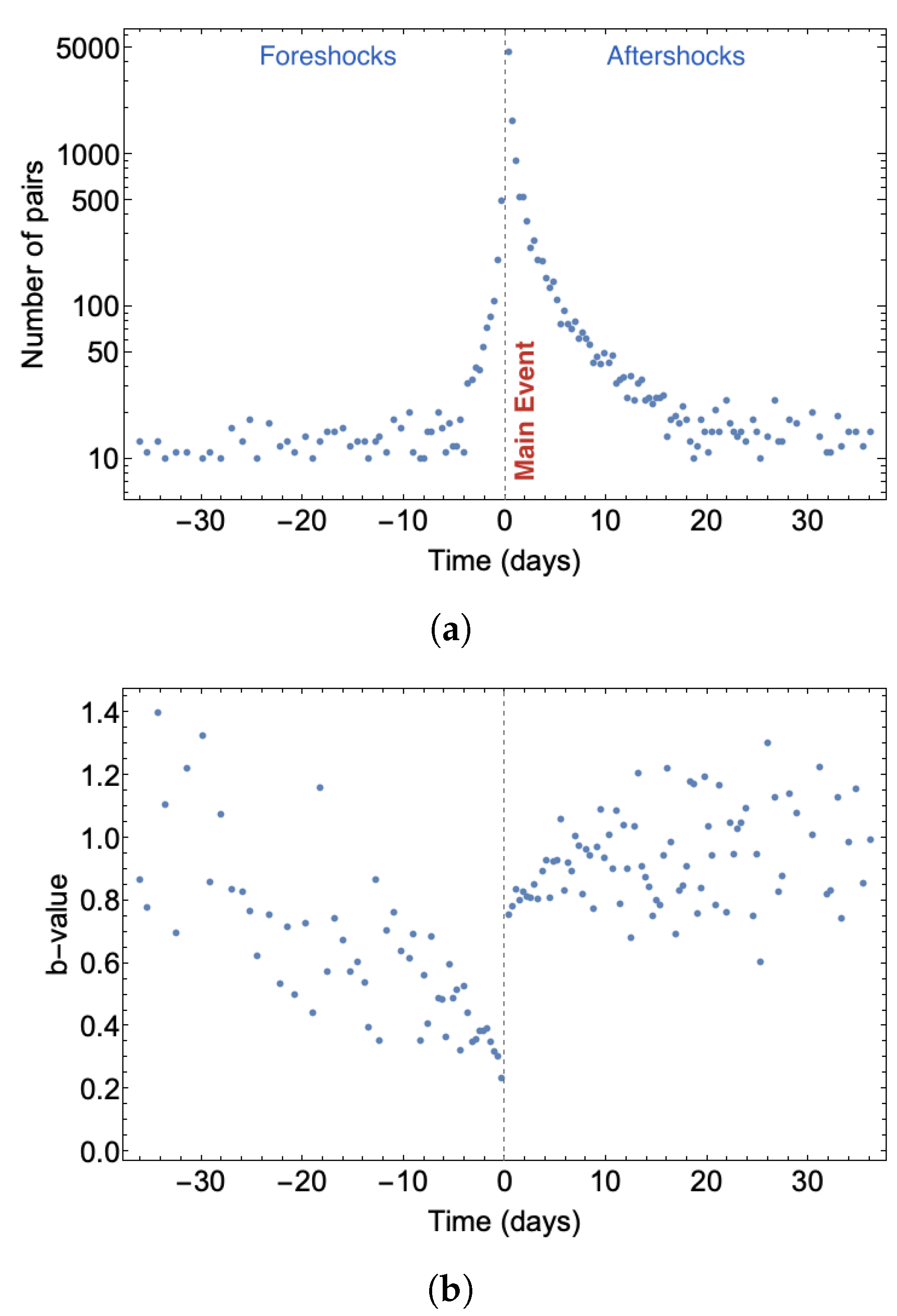
As far as the short-term features are concerned, a clear foreshock and aftershock pattern of the duration of some weeks before and after a magnitude
event is visible in the stacking plot of
Figure 8a. With the same time scale,
Figure 8b shows a clear trend of b-value decreasing before a mainshock of
and recovering to the average value just after it. Note that the large scattering of the b-values has no real physical meaning, but it is simply due to the limited number of earthquakes on which the b-value is calculated. However, this scattering is much smaller just before and after the mainshocks, when the earthquakes rate is much larger. In
Figure S3 of the Supplementary Material, we report the same kind of plots for all the nine combinations of free parameters, showing the same trends, with minor variations. This feature was observed in natural sequences as, for instance, Montuori et al. [
25], Papadopoulos et al. [
26], Gulia and Wiemer [
27].
6. Conclusions
In this study, we assumed a definition of “multiplet” specifically tuned for the application to the seismicity of our study area. A computer code was developed for counting the number of multiplets detected applying such a definition to any earthquake catalog. For the CPTI15 1650–2020 catalog, the code detected eight multiplets, which is a number significantly higher than the average number of multiplets detected in the same way on a set of 500 data sets obtained randomizing the occurrence times of the original catalog (i.e., 4.63 ± 1.88 in
Table 5). The result of this comparison supports the hypothesis that the occurrence of sequences containing multiple mainshocks is not just a casual circumstance. In this study, we also developed a new earthquake simulation code, paying particular attention to the enhancement of stress interaction among rupturing fault elements, and increased the number of multiplets in the simulated catalog. In this way, the number of multiplets detected by the above mentioned computer code on a 100,000-year simulated catalog (176) is 2.13 times higher than the average number of multiplets detected in the same way on a set of 500 randomized catalogs (
Table 5). Besides the production of a significant number of multiplets, the simulated catalog exhibits long- and short-term spatiotemporal features that can be considered realistic imitations of those commonly observed in the real seismicity. We use a stacking procedure in which we compute the number of
events that preceded and followed an
earthquake in bins of five years considering the origin time at the time of every strong event in the 100 kyears simulated catalog. Our results related to northern and central Apennines show an acceleration of seismic activity some centuries before a mainshock, a modest quiescence starting 50 years before the mainshock and a strong aftershock occurrence in the following five years (
Figure 7). In the same way, we analyzed the short term patterns in periods of about one month before and after every
earthquake. Our results confirm the capacity of the simulator code to reproduce typical foreshocks-aftershocks sequences (
Figure 8a). Additionally, in the simulated catalog for northern and central Apennines, the average b-values show a decrease lasting a few weeks before the strong earthquakes, followed by an instantaneous increase at the time of the earthquakes (
Figure 8b). This pattern was observed by Montuori et al. [
25], Papadopoulos et al. [
26], Gulia and Wiemer [
27] in real earthquake sequences.


