Abstract
Suspension bridges and arch bridges are important structural forms of bridges in which the cables are the main load-bearing members. The study of dynamic characteristics of the cable is of great significance to the design and operation and maintenance of suspension bridges and arch bridges. Firstly, this paper derives the cable frequency equation considering the bending stiffness under arbitrary boundary conditions from the dynamic stiffness method (DSM), and gives the calculation method of cable vibration modal frequency based on the W–W algorithm. Secondly, on this basis, the cable boundary condition coefficients and stiffness ratios are introduced to reflect the constraint strength of the main cable and stiffening beam on the cable, so as to study the influence law of these boundary conditions on the cable modal frequency, and then determine the actual cable boundary conditions of this kind of bridge. Finally, the boundary condition coefficients determined in this paper and the relevant parameters of the cables are inversely used to determine the boundary conditions of the actual bridge cables, and a simple method suitable for determining the boundary conditions of the cables in practical engineering is discussed, i.e., the theoretical basis for determining the boundary conditions of the cables through the relevant parameters of the cables, and the practical discussion of the theory is verified through the actual bridge cables. This study provides a reference for further theoretical analysis of cables, a theoretical basis for calculation of actual bridge cables, boundary conditions for in-depth study of dynamic characteristics of cables, and guides the design, operation, and maintenance of cables.
1. Introduction
Bridge cables (stay cables and cables) are an important component of long-span bridges and are widely used in modern engineering. With the increase in the length to slenderness ratio of cables and the decrease in transverse stiffness and internal damping, various types of vibration phenomena are easy to occur under the influence of wind loads and moving loads, etc. [1]. The fatigue caused by cable vibration will cause performance degradation of high-strength steel wire, which will not only further reduce the load-bearing capacity and durability of the cable [2], but also bring a severe test to the safe operation and normal use of cable-stayed bridges, and then affect the driving comfort and even bring visual panic to pedestrians, all of which are inseparable from the dynamics analysis of the cable structure. For cables, the statistical analysis of existing engineering cases shows that the average service life of cables is only ten years [3], and the service life of some cables is even less than ten years. Since the cost of repair and replacement of cables is huge, the importance of their dynamics analysis has far exceeded that of static analysis. The analysis of cable dynamic characteristics has become a key issue in the design, performance monitoring and maintenance, and vibration control of such bridge structures during operation. At the same time, the study of such problems can provide important references for bridge design, internal force distribution in the cable and cable system during service life, and monitoring and evaluation of bridge dynamic characteristics.
At present, the existing dynamic analysis theory of cable structure can be divided into an analytical method, numerical method, and semi-analytical and semi-numerical method according to the analysis method and solution form. In this paper, the dynamic stiffness method is a semi-analytic and semi-numerical method, which starts from the exact vibration function of the system and obtains the frequency equation and dynamic equation in closed form, while using the Euler beam model to model the cable more in line with the real structure. Joseph A. Main [4], in 2007, gave a set of frequency equations to describe the cable system with transverse viscous dampers, which can handle articulated and rigid boundaries, but neglects the effects of sag and inclination. To this end, Dan et al. [5] gave closed-form solutions for the transverse dynamic stiffness of Euler beams with small sag, and also studied the variation law of transverse dynamic stiffness in the spatial and frequency domains. Subsequently, Dan [6] further gave a unified characteristic frequency equation for the structure and its numerical solution under the combined influence of transverse force elements and sag effects. At the same time, based on the PSO (particle swarm optimization) optimization algorithm, he provided a multi-level and multi-parameter identification algorithm suitable for stay cables [7]. Further, Han and Dan [8] used a model of a double-beam system connected by distributed springs to model the composite cable based on the Eulerian beam theory, derived the dynamic stiffness matrix of the model, and studied the influence of parameters such as sag, spring connection layer stiffness, and double-beam flexural stiffness ratio on the modal frequency of the system. At present, for the bare cable system, the existing research work has considered the influence of some factors in the bending stiffness, sag, inclination angle, and internal damping of the cable, but it is not yet possible to consider these factors in a comprehensive manner in an analytical or semi-analytical form. When considering the influence of an elastic support and an elastic embedded boundary at the end of the cable, the existing studies have approximated the vibration function of the cable as the vibration function of the rigidly supported cable. However, the influence of boundary and vibration frequency on the vibration pattern are ignored, so the results are not accurate enough.
The use of the dynamic stiffness method to study the dynamic characteristics of the cable depends largely on the correct judgment of the cable boundary conditions. For the simulation of the boundary conditions of the longer cable, Wang Jun and Duan Bo et al. [9,10] considered the support conditions of both ends of the cable as simple support, and Wei Jiandong and Chen Huai et al. [11,12] considered the support conditions of both ends of the cable as solid support, and their calculation results basically meet the accuracy requirements. However, Xu Xiafei et al. [13] proposed that the influence of the boundary at both ends on the cable frequency is closely related to the cable tension-bending ratio. When studying the dynamic characteristics of the cable, the complex boundary conditions of the actual cable will have a greater impact on the vibration frequency of the cable because the boundary conditions of the cable are not the ideal single simple or solid support.
In view of this, this paper will derive the frequency equation of the cable under each boundary condition by the dynamic stiffness method, and get the actual boundary condition of the cable by proposing the upper and lower limit values of the boundary condition. At the same time, the concepts of boundary condition coefficients and stiffness ratio are introduced in the process of cable modal frequency analysis, and the influence law of these parameters on the cable is studied. Finally, the parameter range for determining the actual boundary conditions of the cables is deduced in the reverse direction with the boundary condition coefficients as the base point, and the research results are applied to the actual bridge cables to provide the theoretical basis of the boundary conditions for the subsequent dynamic characteristics analysis of the cables.
2. Basic Theory of Cable Dynamics Analysis
2.1. Basic Equation and Solution
- (1)
- Basic assumptions and vibration control differential equations.
Taking a single cable as the object of analysis, its simplified model is shown in Figure 1.
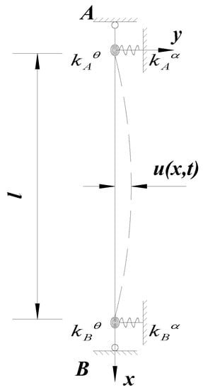
Figure 1.
Analysis model of a single cable.
In order to study the vibration of the single cable shown in Figure 1, the following reasonable assumptions need to be made: (a) the material property of cable is linear elasticity and the cable is always within the range of linear elasticity during the vibration; (b) the strain of the cable is small and its cross-sectional size does not change; (c) the change of the internal tension of the cable along the length of the cable is not considered; (d) the vibration of the cable only occurs in the transverse plane and its vertical axial vibration is neglected; (e) the level of stresses under loads and its influence on vibration in the cable is neglected; and (f) consider the bending stiffness of the cable.
Based on the above basic assumptions, the vibration control differential equations [14] for a transverse unloaded vertical cable with consideration of flexural stiffness in the absence of damping are obtained as follows:
where, is the bending stiffness of the cable; is the transverse displacement function of the cable; is the cable force; is the distance from the upper boundary of the cable; and is the mass per unit length of the cable.
- (2)
- Frequency equation of the cable system
According to the dynamic stiffness theory (DSM) [15], the transverse displacement function of the cable is assumed:
where is the circular frequency (rad/s) and is the time.
Substituting Equation (2) into Equation (1) and the following equation can be obtained:
Introducing dimensionless parameters, , , where is the calculated length of the cable, the dimensionless control differential equation of the system can be obtained by Equation (3):
where, is the ratio of the cable axial force to bending stiffness of the cable and is the dimensionless frequency of the cable.
Thus, the general solution of Equation (4) can be expressed as:
where , , ; and is the fundamental frequency of the cable.
The matrix expression of the general solution (5) is:
where .
According to the relationship between the nodal force and the displacement function of the cable, the nodal displacement of the system represented by the vibration mode function can be obtained.
where and , the specific display expressions are shown in Appendix A. The constant vector can be expressed by Equation (8).
The relationship between the nodal forces and displacements of the cable is:
Taking into account the differences in symbolic conventions, the forces and bending moments at both ends of the cable are expressed as:
Combined with the vibration function expressions in Equations (6) and (8), the following equation can be obtained:
where , the specific explicit expression is shown in the Appendix A.
Thus, the dynamic stiffness matrix is:
where , and the display expressions for each element in are shown in the Appendix A.
The following equation is obtained by boundary conditions of the cable:
Carrying out matrix transformation of Equation (13) leads to:
Then, the following is obtained:
After obtaining the dynamic stiffness matrix of the system, the modal frequencies of the system can usually be solved from the following frequency equation:
where is the value of the determinant.
Finally, the value satisfying the frequency equation of Equation (16) above is exactly the modal frequency of the system.
2.2. Description of the Single Cable Boundary Constraint
Since the transverse and vertical directions of the cable are not coupled with each other, the influence of the vertical support constraint on the transverse vibration of the cable can be neglected when studying the transverse vibration of a single cable. In the transverse boundary conditions, it can be assumed that the transverse bearing displacement stiffness and at both ends, and the corner stiffness and can be arbitrary values, that is, it is the composite boundary condition considering the actual situation, then Equation (14) can be transformed into the following equation:
where, the expressions , and are shown in the Appendix A.
Through the analysis of the calculation examples in the literature [13], it is reliable to propose that the tension-bending ratio is used to measure the influence of the boundary conditions on the dynamic characteristics of the cable. When the tension-bending ratio is , the influence of the boundary conditions at both ends of the cable on the cable frequency can be neglected; however, when the tension-bending ratio is , the influence of the actual boundary conditions must be considered for the calculation of the cable. Here, we only discuss and analyze the single cable boundary conditions for the tension-bend ratio of .
According to the relative values between the flexural stiffness of the cable and the boundary conditions, the dimensionless boundary condition coefficients and are introduced, where:
In practice, the boundary condition of the cable is between simple and solid support, i.e., and can be any value in the interval [0, 1].
Where, the corner stiffness can be expressed by the boundary condition coefficient from Equation (18), i.e.,
Substituting Equation (19) into the frequency Equation (17) yields the cable frequency equation considering the boundary condition coefficients.
2.3. Solution of Dynamic Characteristics
The above frequency Equations (14) and (20) can be used to calculate the dynamic characteristics of bridge cables. Obviously, both forms of frequency equations are complex transcendental equations, and ordinary algorithms for solving them will encounter difficulties, high computational effort, and low accuracy, or even loss of modalities. Therefore, in this paper, the Wittrick–Williams (W–W) algorithm [16] is chosen for the calculation of cable frequencies, which can solve the cable frequency equation accurately and efficiently.
The W–W algorithm is not directly used for frequency calculation, but obtains the number of modal frequencies of the structure less than the trial frequency by counting, so that the upper and lower bounds of arbitrary order frequencies can be determined. Finally, the frequency solution of arbitrary accuracy can be obtained by combining the dichotomous method or Newton’s method. Since this method allows the dynamic stiffness matrix to maintain the Sturm sequence properties, it can ensure that no roots are missed during the solution of the equation, and its stability and correctness have been proved theoretically, which is an advantage that most analytical and approximate solution methods do not have [16]. The key step in applying the W–W algorithm to calculate the structural modal frequency problem is to determine the modal frequency count of the structure, which represents the number of modal frequencies of the structure less than :
where, is the count related to the overall dynamic stiffness matrix of the structure, which is equal to the number of negative elements on the main diagonal of the triangular matrix ; is the upper triangular matrix formed by the Gauss elimination of the dynamic stiffness matrix of the structure; is the count symbol; and is the count of the solid end frequency of the structure, which is equal to the number of solid end frequencies of the structure less than the trial frequency . The solid end frequency of the structure is the modal frequency after the boundary conditions of the structure are all solidified, which may be called the solid end structure corresponding to the original structure.
After calculating the solid end frequency count of the structure under the trial frequency , the number of modal frequencies of the structure less than the trial frequency can be calculated according to Equation (21). Thereafter, after first roughly determining the upper and lower bounds and of the modal frequency of that order, the i-th order modal frequency of the structure can be calculated, so that it satisfies:
The i-th order modal frequency of the structure satisfies , and thereafter the dichotomous method [17] can be used to approach the true frequency by continuously adjusting the values of the upper and lower bounds. When is met, the modal frequency within the allowable error range can be obtained. In this paper, the method is used to write a program to solve the modal frequencies of each order of the cable.
2.4. Method Validation
The method in this paper is verified by combining the analysis process of elastic boundary conditions considering beam axial forces in the literature [18], and the frequency calculation Equation (9) shown as Equation (23) in this literature is used to calculate the frequency values of the cable under the boundary conditions in this paper. From the dimensionless parameter in this paper, the rotational stiffnesses of the boundary conditions at the both ends of the corresponding cable can be determined. Taking as 1.0, 10, 100, and , respectively, the corresponding boundary condition coefficient values can be obtained. Taking a cable as an example, its material characteristics are: free length of the cable , modulus of elasticity , bending moment of inertia , line mass per unit length , and cable force .
where, , , , , , , , .
Using the dynamic stiffness method and the W–W algorithm, the frequency value of the cable under the corresponding boundary condition coefficient is calculated by programming and compared with the frequency calculated by using the elastic boundary condition formula in the literature. The calculation results are shown in Table 1. In order to verify the accuracy of the method for calculating the cable frequencies and the definition of the boundaries by the boundary condition coefficients, the relative errors between the calculated values in this paper and the calculated values in the literature were analyzed, and each relative error values are included in Table 1.

Table 1.
Frequency error analysis.
From the calculation results and error analysis in Table 1, it can be seen that through the comparison of calculation results, the maximum relative error between the existing literature and the theory of this paper in calculating the order frequencies of cables under different boundary conditions is no more than 1.5%. The error analysis shows that the results calculated by the method of this paper are very close to the order frequencies calculated by the literature, that is, under the premise that the accuracy of the calculation method of the literature has been verified, the method of this paper can be used to accurately calculate the modal frequencies of each order of the cable under each boundary condition, which greatly verifies the accuracy of the theoretical analysis and calculation method of this paper providing an accurate theoretical basis for further calculation of the cable.
3. Effect of Boundary Conditions on Dynamic Characteristics of Cable
3.1. Effect of Changing Boundary Conditions on Frequency
- (1)
- Ideal state equality boundary
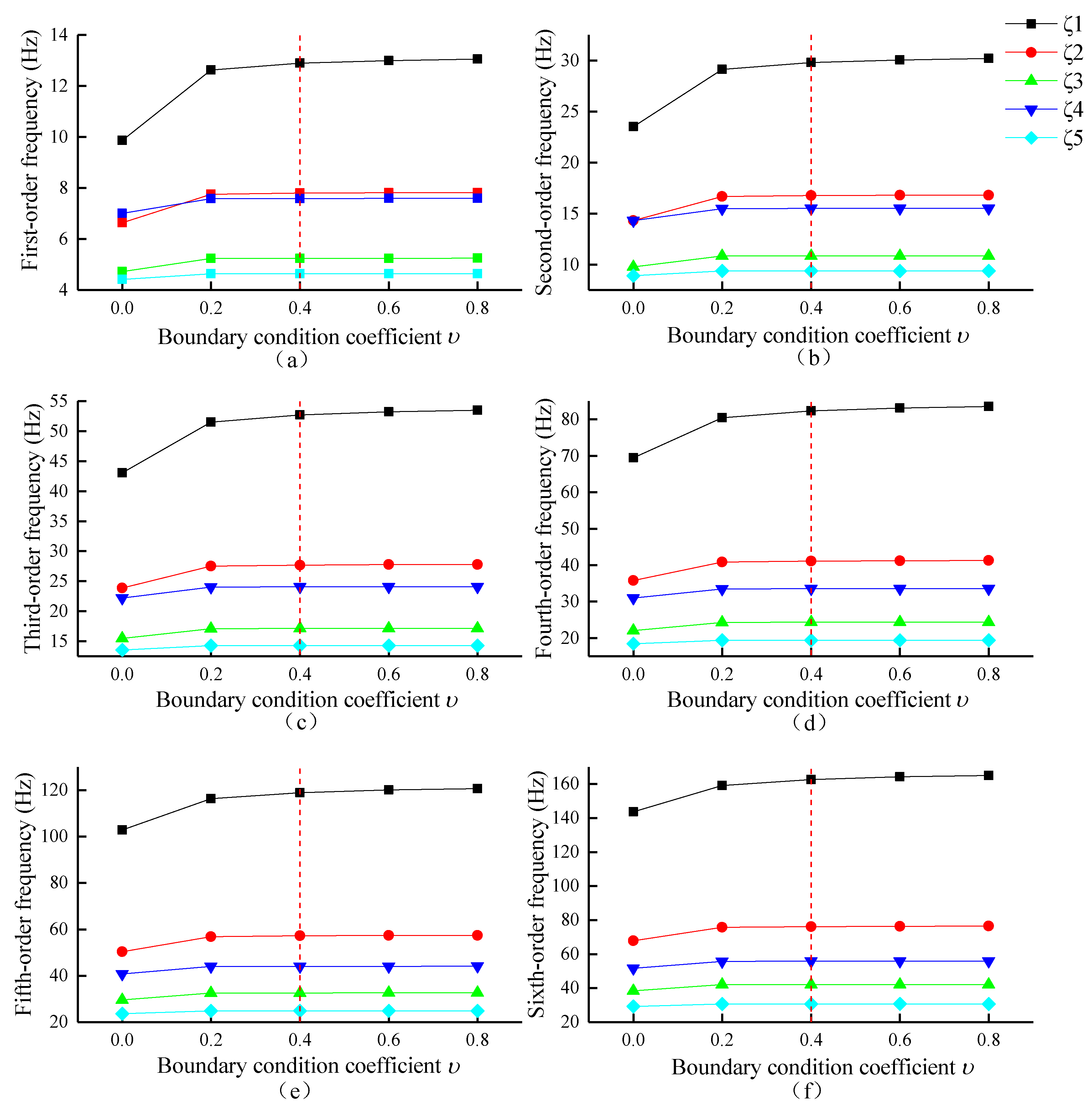
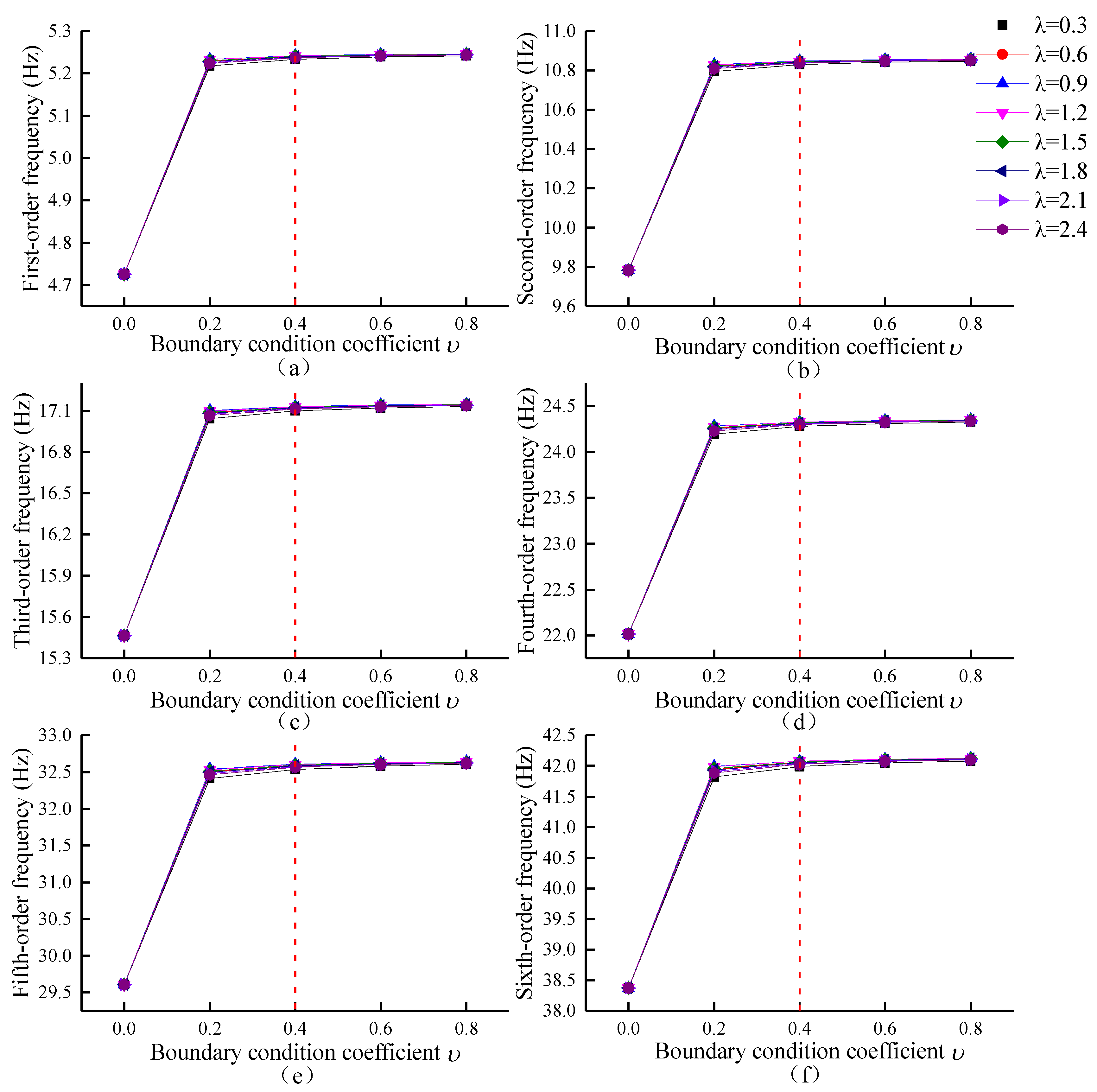
In the ideal state, the main cable stiffness and stiffening beam stiffness are considered to be nearly the same, that is, assuming that and are 0, 0.2, 0.4, 0.6, and 0.8, respectively, the rotational stiffness at both ends of the corresponding boundary becomes larger from 0, and the boundary conditions at both ends of the cable evolve gradually from simple to solid support.
The cable parameters are shown in Table 2 for five cables of different lengths arbitrarily.
Table 2.
Cable parameters.
Using the cable frequency calculation method in this paper, the frequency variation of each cable under different boundary condition coefficients is studied and plotted as a curve, as shown in Figure 2.
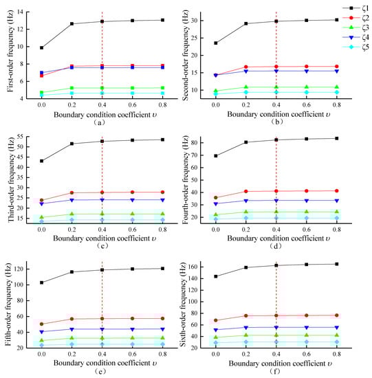
Figure 2.
Variation of each order frequency of each cable under equal boundary conditions: (a) to (f) denote the variation of the first to sixth order frequencies of each cable under equal boundary conditions with different boundary condition coefficients, respectively.
From Figure 2, it can be obtained that in the process of changing the boundary condition coefficient, the change trend of each order frequency of cables with different tension-bending ratios is almost the same but with the increase in the tension-bending ratio , the change of each order frequency of cables from simple support to solid support is less obvious. When the tension-bending ratio is , the change of frequency of cables with boundary conditions is more obvious. During the change of boundary condition coefficient, when , with the increase in the boundary condition coefficient at both ends, each order frequency of each cable basically remains the same. At this time, both ends of the boundary have tended to solid support, that is, when the boundary condition coefficient is 0.4, the upper and lower boundaries of the cable can be treated as the solid support boundary.
- (2)
- Actual non-equal boundary
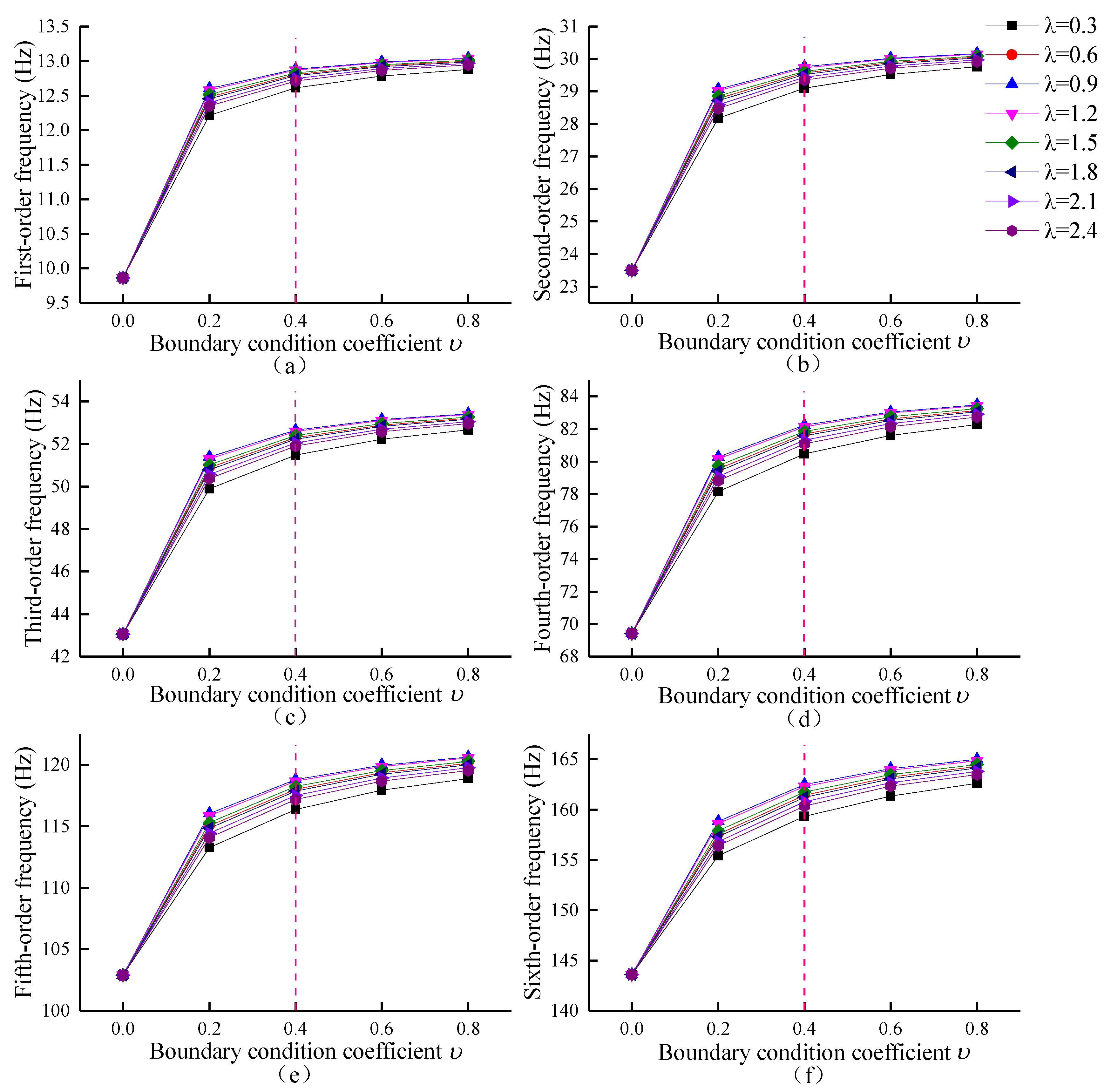
In actual engineering, the constraints of suspension bridge main cable and stiffening beam on the cable, or arch bridge, arch rib, and tie beam on the cable are different. Therefore, a material influence coefficient is introduced, where is the ratio of the stiffness of the main cable to the stiffening beam of a suspension bridge (or the ratio of the stiffness of the arch rib to the stiffness of the tie beam of an arch bridge), referred to as the stiffness ratio, i.e., . Reinforced concrete and steel are the main materials used for stiffened girders in suspension bridges, but the materials can vary from plain concrete to steel. The flexural stiffness of plain concrete and reinforced concrete stiffening beam is less than the stiffness of the main cable with strong tensile reserves, and the impact of the flexural stiffness of this kind of stiffening beams is only of secondary importance to the structural behavior of the whole bridge, while the flexural stiffness of the steel stiffening beam is significantly greater than the flexural stiffness of the main cable made of steel strands. For the now commonly used parallel steel wire main cable, the research [19] shows that its internal structure is closest to that of a semi-parallel steel wire cable, and its flexural stiffness is 0.37 times that of the steel strand. According to the calculation and analysis of relevant data and the limit value in the design code [20], the upper and lower limits of the material influence coefficient can be roughly determined, i.e., . starting from 0.3 to vary in steps of 0.3, when , is taken as 0, 0.2, 0.4, 0.6, and 0.8, respectively; when , is taken as 0, 0.2, 0.4, 0.6, and 0.8, respectively.
Using the calculation method in this paper, the frequency variation graphs of each order of #1 cable and #4 cable under different stiffness ratios in Table 2 above are obtained, as shown in Figure 3 and Figure 4.
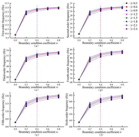
Figure 3.
The #1 cable frequency variation of each order: (a) to (f) are the variations of the first to sixth order frequencies of #1 cable under different boundary condition coefficients for each material influence factor, respectively.
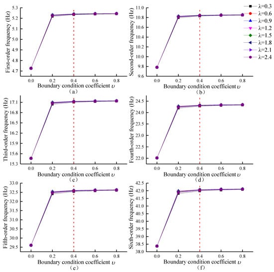
Figure 4.
The #4 cable frequency variation of each order: (a) to (f) are the variations of the first to sixth order frequencies of #4 cable under different boundary condition coefficients for each material influence factor, respectively.
From Figure 3 and Figure 4, it can be seen that no matter how the material influence coefficient changes, when the boundary condition coefficient or reaches 0.4, boundaries at both ends can reach the solid support boundary, and under different material influence coefficients, the change trend of each order frequency of the cable with the change of boundary conditions tends to be the same. In the variation diagram of each order frequency of the cable, with the increase in the material influence coefficient , each order frequency of the cable increases slightly; however, with the increase in the tension-bending ratio of the cable, this change trend is close to zero, that is, the influence of the material influence coefficient on the frequency of the cable can be ignored. At the same time, when the material influence coefficient is the ideal equal boundary condition , the relevant conclusions obtained are consistent with this analysis, that is, in actual engineering, it is not necessary to consider the stiffness ratio of the upper and lower boundaries of the cable, and the two ends of the cable can be treated as equal boundaries.
3.2. Accuracy Verification of Boundary Condition Range
The validation example in the literature [21] is selected to verify the conclusions of this paper. In this literature, a suspender with fixed boundaries at both ends is selected, and its free length , elastic modulus , section moment of inertia , linear mass per unit length , and suspender axial force are known. The method in this paper is used to calculate the frequency value when the boundary condition coefficient is 0.4. Here, due to symmetry, the stiffness ratios are 0.3 and 1.0, respectively. In order to verify the accuracy of defining the fixed support with the determined boundary condition coefficients, the relative errors between the suspender frequency values calculated in this paper and the measured values under the fixed support are compared, and the results of the calculation are shown in Table 3.
Table 3.
Comparison analysis of measured and calculated frequencies.
It can be clearly seen from Table 3 that this paper uses the value of the boundary condition coefficient to define the cable boundary with sufficient accuracy. The determination of the boundary conditions is independent of the stiffness ratio , as the upper and lower boundary stiffnesses of the cable are reciprocal, the cable ends will be solidly supported when any of the boundary condition coefficients reaches 0.4. Similarly, in a single cable, the value of the corner stiffness can be determined by the boundary condition coefficient , from Equation (20), can be obtained by . When , both ends of the cable are simply supported; when , both ends of the cable are solidly supported, replacing the theoretical condition of the cable being solidly supported.
4. Application Discussion
4.1. Discussion
In the cable performance analysis, the cable boundary conditions have a great influence on the dynamic characteristics of the cable, while the cable stiffness ratio has a negligible effect on them. Since only the axial force of the cable is considered, the conclusions of the studied cable-related boundary conditions of suspension bridges can be extended to arch bridge booms and other bridge cables. In order to make the research results better applied to the engineering practice, further derivation is needed. Then, the actual boundary conditions of relevant parameter cables are inversely obtained by using the defined range of boundary condition coefficients, which is convenient for the study of dynamic characteristics of cables in practical engineering.
Previous studies have shown that the effect of cable boundary conditions on the cable gradually decreases as the tension-bending ratio increases [14]. When the tension-bending ratio is , the influence of the boundary conditions at both ends of the cable on the cable frequency can be neglected, but when the tension-bending ratio is , the calculation of the cable must consider the influence of the actual boundary conditions. Therefore, it can be concluded that when the tension-bending ratio is , the two ends of the cable with the tension-bending ratio of obtained from the definition of the tension-bending ratio can be calculated with simple support or fixed support. However, due to the convenience of the actual calculation, it is recommended to give preference to the simple support boundary.
This paper mainly analyzes the cable with the tension-bending ratio of . The research results show that when the cable boundary condition coefficient is , i.e., , the two ends of the cable can be treated as the solid support boundary and the cable frequency changes more obviously with the boundary condition when the cable tension-bending ratio is obtained from the above analysis. Therefore, substituting , , and into Equation (20) can get , that is, the boundary conditions of both ends of the cable with shall be treated as a solid support boundary. However, in the case of the simple and solid support, it is recommended that the boundary of both ends of the cable with shall be treated as the elastic complex boundary.
Therefore, in practical engineering, we can start from the parameters of the cable, compare the relationship between the cable length, stiffness, and cable force, and then determine the boundary conditions of each cable of the bridge, which avoids the tedious analysis of determining the boundary conditions of the cable in practical engineering, provides convenience for the calculation of cable characteristics in practical engineering, and provides a boundary condition basis for further theoretical analysis of the cable.
4.2. Discussion Application
- (1)
- Engineering background
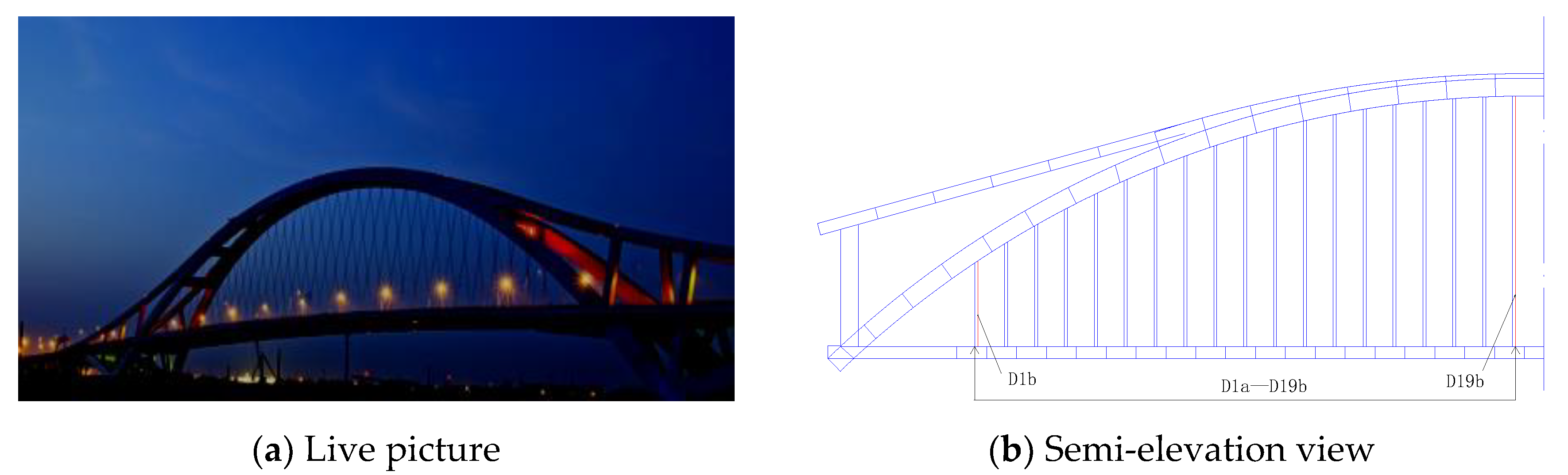
Project 1: Mingzhou Bridge shown in Figure 5 is located on the waterway of the Yongjiang River and its main bridge is a 100 + 450 + 100 m double-limb center-beam steel box arch bridge. There are 38 pairs of mid-span cables with 9 m spacing in the same plane with the arch ribs. A total of four groups of side cables are made of parallel steel wire cables of 199Φ5, and the remaining 34 groups of mid-span cables are made of parallel steel wire cables of 91Φ5; both ends of the cables are anchored by cold casting, and the cables are tensioned at the top of the arch. The stiffeners are supported on the arch ribs by suspenders or columns, and the two ends of the mid-span stiffeners are supported on the crossbeam at the intersection of the mid-span arch beams, with expansion joints at both ends of the stiffeners and longitudinal sliding bearings at the end supports, and damping limit devices set horizontally and longitudinally.
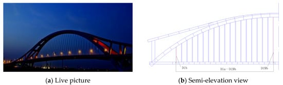
Figure 5.
Mingzhou Bridge.
Project 2: Sanshan West Bridge shown in Figure 6 is located at the intersection of the Pingzhou waterway and the Pearl Zhujiang waterway with a main span of 200 m. The main arch rib is composed of two 4Φ750 steel pipe concrete, connected by plate embellishment strips to form a steel pipe concrete lattice column. In the section from the first suspender to the foot of the arch, there are nine parallel cross braces, each of which is a truss beam made of empty steel pipes. The whole structure uses the self-weight of the side span to balance the huge thrust of the main arch through the floating flexible structure, so that the side span, the main span, and the lower foundation can be deformed and stressed together.
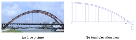
Figure 6.
Sanshan West Bridge.
- (2)
- Application verification
In order to apply the above engineering discussion to the actual bridge project, two representative cables, D1b and D19b, on the Mingzhou Bridge shown in Figure 5 and the C33 suspender on the Sanshan West Bridge shown in Figure 6 were selected as the verification objects for the discussion. The basic parameters of cables and suspenders are shown in Table 4. The error between the corresponding frequency values calculated by the analysis of various boundary conditions and the actually measured frequency values was analyzed, and the results are shown in Table 5. The discussion in this paper is preliminarily applied to the actual bridge engineering, and the accuracy of the boundary conditions at both ends of the cable defined by the cable length is tested to a certain extent.
Table 4.
Basic parameters of each cable.
Table 5.
Comparison of the frequency values of each cable.
As can be seen from Table 5, for the cables with , the boundary conditions have little effect on their frequencies, but for the cables with , the frequencies calculated by applying the fixed support boundary conditions are closer to the frequency values in actual engineering, while for the cables with a length between the two, it is recommended to treat both ends as elastic boundaries. By calculating the frequency values of the cables under the three different boundary conditions and comparing them with their measured frequency values, it is verified that the discussion of determining the boundary conditions of the corresponding cables from the corresponding cable length range proposed in this paper has a certain accuracy. The determination of cable boundary conditions by cable length has guiding significance in the analysis of cable dynamic characteristics. From the basic calculation of cable frequency to the measurement of cable force in the process of cable use, the determination of boundary conditions can clarify the application scope of previous formulas, solve the basic problem of difficult calculation of cable frequency in engineering practice, and provide a new way for its accurate test and calculation. The analysis can be applied in cable-stayed, short suspenders of arch bridges and other structures; however, determining the length of the cable in the elastic boundary needs further discussion.
5. Conclusions
This paper starts from the dynamic stiffness theory, and uses the W–W algorithm as the basis to calculate and analyze the influence of the cable boundary conditions on the cable frequency with the tension-bending ratio using programming language. At the same time, this paper describes the boundary conditions with the boundary condition coefficients, analyzes the influence of each boundary condition on the cable frequency, and extends it to the engineering practice in reverse and puts forward the discussion of determining the boundary conditions with the cable parameters, which provides the cornerstone for the subsequent research. This paper has the following main conclusions.
- (1)
- The analysis of the results of this paper shows that the influence of the stiffness ratio of the upper and lower boundary of the bridge cable on the cable frequency is negligible, and only the influence of the change of the boundary coefficient on the cable frequency needs to be considered.
- (2)
- The boundary condition coefficient is used to describe the cable boundary condition with a certain accuracy, and the actual boundary condition coefficient in this paper can be used to replace the simple and fixed support conditions in the theory. When the cable vibrates transversely and the displacement stiffness of the lateral support at both ends is infinite, the boundary condition coefficient of both ends of the cable reaches 0.4 from 0, and the two ends of the cable change from simple support to fixed support, that is, the rotational stiffness of the cable is , which replaces the case of judging the boundary condition by in the theory.
- (3)
- In actual engineering, the boundary conditions of the cable can be determined from the cable parameters. Both ends of the cable with can be calculated by using simple support boundary; when , the boundary conditions at both ends of the cable shall be treated as a fixed support boundary; when , the boundary at both ends of the cable shall be treated as an elastic complex boundary.
Through the analysis of the dynamic characteristics of the cable—from defining the boundary conditions of the cable with the boundary condition coefficient to the correct application of the cable boundary conditions in practical engineering—this paper verifies the accuracy with the literature and measured data, which can determine the cable boundary conditions on the basis of the cable parameters, providing a reference basis for the study of the dynamic characteristics of the cable and the health monitoring of the actual cable.
Author Contributions
Conceptualization, D.D. and F.H.; methodology, X.L.; software, X.L.; validation, D.D., X.L. and F.H.; formal analysis, X.L.; investigation, X.L.; resources, D.D.; data curation, D.D., X.L. and F.H.; writing—original draft preparation, X.L.; writing—review and editing, D.D. and X.L.; visualization, X.L.; supervision, D.D. and F.H.; project administration, D.D.; funding acquisition, D.D. All authors have read and agreed to the published version of the manuscript.
Funding
This research received no external funding.
Data Availability Statement
Some or all data, models, or code that support the findings of this study are available from the corresponding author upon reasonable request.
Acknowledgments
This work was supported by the Xinjiang University Tianshan Scholar Distinguished Professor Research Start-up Fund (grant numbers 620312327).
Conflicts of Interest
The authors declare no conflict of interest.
Appendix A
References
- Fujino, Y.; Kimura, K.; Tanaka, H. Wind Resistant Design of Bridges in Japan; Springer: Tokyo, Japan, 2014. [Google Scholar]
- Dan, D.; Sun, L.; Guo, Y.; Cheng, W. Study on the Mechanical Properties of Stay Cable HDPE Sheathing Fatigue in Dynamic Bridge Environments. Polymers 2015, 7, 1564–1576. [Google Scholar] [CrossRef] [Green Version]
- Furuya, K.; Kitagawa, M.; Nakamura, S.I.; Suzumura, K. Corrosion Mechanism and Protection Methods for Suspension Bridge Cables. Struct. Eng. Int. 2000, 10, 189–193. [Google Scholar] [CrossRef]
- Main, J.A.; Jones, N.P. Vibration of Tensioned Beams with Intermediate Damper. I: Formulation, Influence of Damper Location. J. Eng. Mech. 2007, 133, 369–378. [Google Scholar] [CrossRef] [Green Version]
- Dan, D.; Xu, B.; Huang, H.; Yan, X.F. Research on the characteristics of transverse dynamic stiffness of an inclined shallow cable. J. Vib. Control 2014, 22, 1609–1610. [Google Scholar] [CrossRef]
- Dan, H.D.; Xu, B.; Chen, Z.H. Universal Characteristic Frequency Equation for Cable Transverse Component System and Its Universal Numerical Solution. J. Eng. Mech. 2016, 142, 4015105. [Google Scholar] [CrossRef]
- Dan, D.H.; Xia, Y.; Xu, B.; Han, F.; Yan, X.F. Multistep and Multiparameter Identification Method for Bridge Cable Systems. J. Bridge Eng. 2018, 23, 04017111. [Google Scholar] [CrossRef]
- Fei, H.; Danhui, D.; Cheng, W.; Jia, P. Analysis on the dynamic characteristic of a tensioned double-beam system with a semi theoretical semi numerical method. Compos. Struct. 2017, 185, 584–599. [Google Scholar] [CrossRef]
- Wang, J.; Wang, F.; Zhou, X. Research on cable force testing of cable-stayed bridges based on fluctuation method. J. Appl. Sci. 2005, 23, 90–93. [Google Scholar]
- Duan, B.; Zeng, D.; Lu, J. Analysis on cable force measurement of cable-stayed bridge. J. Chongqing Jiaotong Univ. 2005, 24, 6–9. [Google Scholar]
- Wei, J. Accuracy analysis of common formulas for cable force measurement. Highw. Traffic Sci. Technol. 2004, 21, 53–56. [Google Scholar]
- Chen, H.; Dong, J.-H. Practical formula of vibration method for determination of sling tension in medium and lower bearing arch bridges. Chin. J. Highw. 2007, 20, 66–70. [Google Scholar]
- Xu, X.; Ren, W. Influence of boundary conditions on the estimation of sling force. J. Railw. Sci. Eng. 2008, 06, 26–31. [Google Scholar]
- Humar, J.L. Dynamics of Structures; Prentice-Hall, Inc.: Englewood Cliffs, NJ, USA, 1990. [Google Scholar]
- Banerjee, J.R. Dynamic stiffness formulation for structural elements: A general approach. Comput. Struct. 1997, 63, 101–103. [Google Scholar] [CrossRef]
- Williams, F.W.; Wittrick, W.H. An automatic computational procedure for calculating natural frequencies of skeletal structures. Int. J. Mech. Sci. 1970, 12, 781–791. [Google Scholar] [CrossRef]
- Wittrick, W.H.; Williams, F.W. A general algorithm for computing natural frequencies of elastic structures. Q. J. Mech. Appl. Math. 1971, 24, 263–284. [Google Scholar] [CrossRef]
- Xing, J.Z.; Wang, Y.G. Free vibrations of a beam with elastic end restraints subject to a constant axial load. Arch. Appl. Mech. 2013, 83, 241–252. [Google Scholar] [CrossRef]
- Su, C.; Xu, Y.F.; Han, D.J. Parameter analysis and identification of bending stiffness of cables in measuring cable force by the frequency method. Highw. Traffic Technol. 2005, 22, 75–78. [Google Scholar]
- Lei, J. Suspension Bridge Design; People’s Traffic Press: Beijing, China, 2002. [Google Scholar]
- Gan, Q. Study on Internal Force Identification Method of Cable Structure under Complex Boundary Conditions; South China University of Technology: Guangzhou, China, 2015. [Google Scholar]


Publisher’s Note: MDPI stays neutral with regard to jurisdictional claims in published maps and institutional affiliations. |
© 2022 by the authors. Licensee MDPI, Basel, Switzerland. This article is an open access article distributed under the terms and conditions of the Creative Commons Attribution (CC BY) license (https://creativecommons.org/licenses/by/4.0/).