
Modeling Random Exit Selection in Intercity Expressway Traffic with Quantum Walk


Abstract
:1. Introduction
2. Problem Definition and Basic Idea
2.1. Formal Definition of the Problem
2.2. Basic Idea
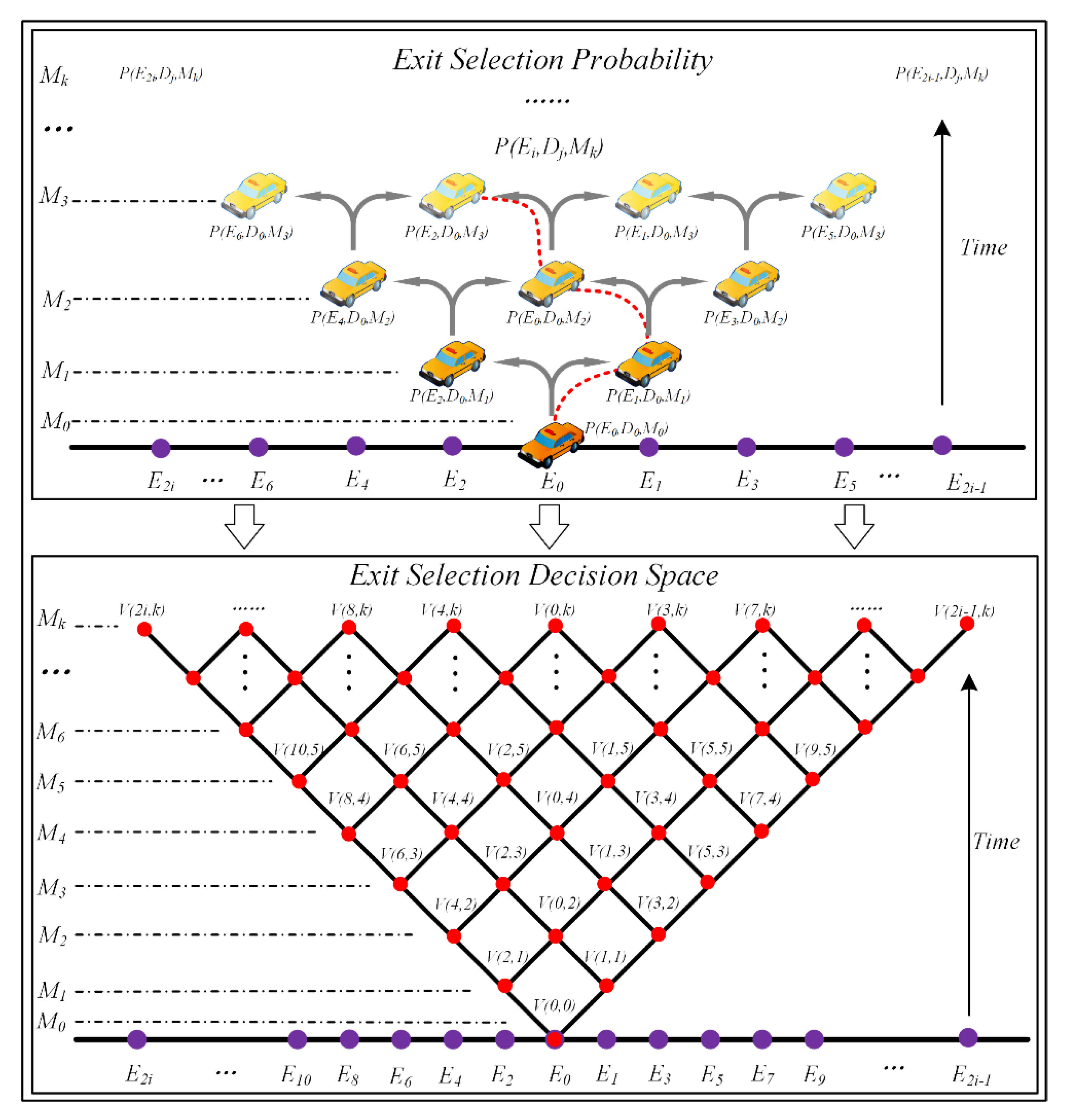
3. The RQTM Model
3.1. Quantum Walk Simulation of Random Exit Selection
3.2. Map Probability Dynamics to Traffic Volumes
4. Experiments
4.1. Research Data and Experiment Configuration
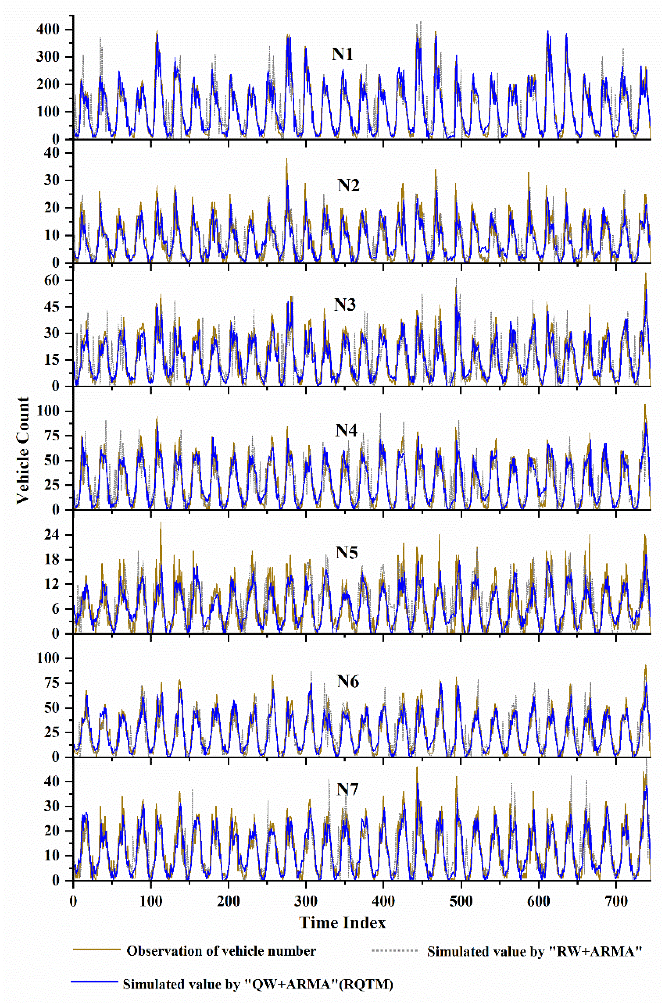
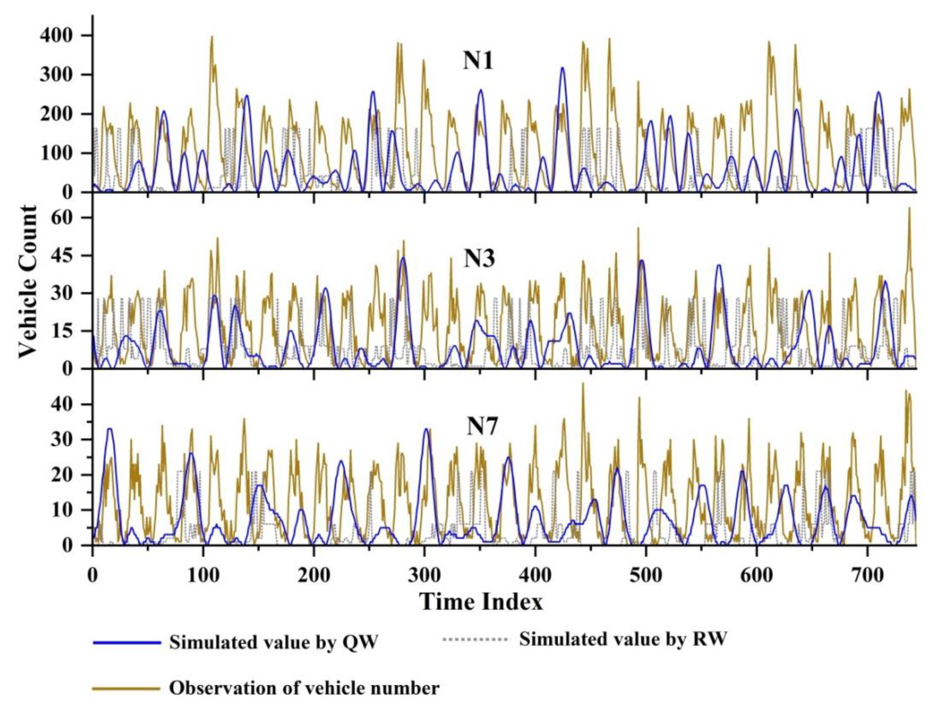
4.2. Results
5. Discussion
5.1. Improvement of Modeling Fikr over Classical Random Walk
5.2. Applicable Issues and Future Works of Quantum Walk
6. Conclusions
Author Contributions
Funding
Institutional Review Board Statement
Informed Consent Statement
Data Availability Statement
Conflicts of Interest
References
- Jiang, R.; Wu, Q.; Zhu, Z. Full velocity difference model for a car-following theory. Phys. Rev. E 2001, 64, 17101. [Google Scholar] [CrossRef] [PubMed] [Green Version]
- Ramezani, M.; Geroliminis, N. On the estimation of arterial route travel time distribution with Markov chains. Transp. Res. Part B Methodol. 2012, 46, 1576–1590. [Google Scholar] [CrossRef] [Green Version]
- Ermagun, A.; Levinson, D. Spatiotemporal traffic forecasting: Review and proposed directions. Transp. Rev. 2018, 38, 786–814. [Google Scholar] [CrossRef]
- Seo, T.; Bayen, A.M.; Kusakabe, T.; Asakura, Y. Traffic state estimation on highway: A comprehensive survey. Annu. Rev. Control 2017, 43, 128–151. [Google Scholar] [CrossRef] [Green Version]
- Bekiaris-Liberis, N.; Roncoli, C.; Papageorgiou, M. Highway traffic state estimation with mixed connected and conventional vehicles. IEEE Trans. Intell. Transp. Syst. 2016, 17, 3484–3497. [Google Scholar] [CrossRef] [Green Version]
- Chen, R.B. Models of Count with Endogenous Choices. Transp. Res. Procedia 2017, 23, 460–479. [Google Scholar] [CrossRef]
- Bekhor, S.; Prashker, J.N. GEV-based destination choice models that account for unobserved similarities among alternatives. Transp. Res. Part B Methodol. 2008, 42, 243–262. [Google Scholar] [CrossRef]
- Danial, A.; Ali, A.A.; Mohammad, S. Prediction of vessels locations and maritime traffic using similarity measurement of trajectory, Ann. GIS 2021, 27, 151–162. [Google Scholar] [CrossRef]
- Tolouei, R.; Psarras, S.; Prince, R. Origin-Destination trip matrix development: Conventional methods versus mobile phone data. Transp. Res. Procedia 2017, 26, 39–52. [Google Scholar] [CrossRef]
- Yuan, Y.; Van Lint, J.W.C.; Wilson, R.E.; Van Wageningen-Kessels, F.; Hoogendoorn, S.P. Real-time lagrangian traffic state estimator for freeways. IEEE Trans. Intell. Transp. Syst. 2012, 13, 59–70. [Google Scholar] [CrossRef]
- Xu, C.; Li, Z.; Wang, W. Short-term traffic flow prediction using a methodology based on autoregressive integrated moving average and genetic programming. Transport 2016, 31, 343–358. [Google Scholar] [CrossRef] [Green Version]
- Haddad, J.; Ramezani, M.; Geroliminis, N. Cooperative traffic control of a mixed network with two urban regions and a freeway. Transp. Res. Part B Methodol. 2013, 54, 17–36. [Google Scholar] [CrossRef] [Green Version]
- Adacher, L.; Tiriolo, M. A macroscopic model with the advantages of microscopic model: A review of Cell Transmission Model’s extensions for urban traffic networks. Simul. Model. Pract. Theory 2018, 86, 102–119. [Google Scholar] [CrossRef]
- Barlovic, R.; Schadschneider, A.; Schreckenberg, M. Random walk theory of jamming in a cellular automaton model for traffic flow. Phys. A Stat. Mech. Its Appl. 2001, 294, 525–538. [Google Scholar] [CrossRef] [Green Version]
- González, M.C.; Hidalgo, C.A.; Barabási, A.L. Understanding individual human mobility patterns. Nature 2008, 453, 779–782. [Google Scholar] [CrossRef]
- Szell, M.; Sinatra, R.; Petri, G.; Thurner, S.; Latora, V. Understanding mobility in a social petri dish. Sci. Rep. 2012, 2, 457. [Google Scholar] [CrossRef]
- Zhu, J.; Ye, X. Development of destination choice model with pairwise district-level constants using taxi GPS data. Transp. Res. Part C Emerg. Technol. 2018, 93, 410–424. [Google Scholar] [CrossRef]
- Hasnat, M.M.; Faghih-Imani, A.; Eluru, N.; Hasan, S. Destination choice modeling using location-based social media data. J. Choice Model. 2019, 31, 22–34. [Google Scholar] [CrossRef]
- Qu, X.; Zhang, J.; Wang, S. On the stochastic fundamental diagram for freeway traffic: Model development, analytical properties, validation, and extensive applications. Transp. Res. Part B Methodol. 2017, 104, 256–271. [Google Scholar] [CrossRef]
- Gao, S.; Li, M.; Liang, Y.; Marks, J.; Kang, Y.; Li, M. Predicting the spatiotemporal legality of on-street parking using open data and machine learning. Ann. GIS 2019, 25, 299–312. [Google Scholar] [CrossRef]
- Calabrese, F.; Colonna, M.; Lovisolo, P.; Parata, D.; Ratti, C. Real-time urban monitoring using cell phones: A case study in Rome. IEEE Trans. Intell. Transp. Syst. 2011, 12, 141–151. [Google Scholar] [CrossRef]
- Song, C.; Koren, T.; Wang, P.; Barabási, A.-L. Modelling the scaling properties of human mobility. Nat. Phys. 2010, 6, 818–823. [Google Scholar] [CrossRef] [Green Version]
- Zhao, X.; Wan, C.; Sun, H.; Xie, D.; Gao, Z. Dynamic rerouting behavior and its impact on dynamic traffic patterns. IEEE Trans. Intell. Transp. Syst. 2017, 18, 2763–2779. [Google Scholar] [CrossRef]
- Zeng, G.; Li, D.; Guo, S.; Gao, L.; Gao, Z.; Stanley, H.E.; Havlin, S. Switch between critical percolation modes in city traffic dynamics. Proc. Natl. Acad. Sci. USA 2019, 116, 23–28. [Google Scholar] [CrossRef] [PubMed] [Green Version]
- Simini, F.; González, M.C.; Maritan, A.; Barabási, A.-L. A universal model for mobility and migration patterns. Nature 2012, 484, 96–100. [Google Scholar] [CrossRef] [PubMed]
- Yan, X.-Y.; Wang, W.-X.; Gao, Z.-Y.; Lai, Y.-C. Universal model of individual and population mobility on diverse spatial scales. Nat. Commun. 2017, 8, 1639. [Google Scholar] [CrossRef] [PubMed] [Green Version]
- Sheu, J.B. Characterisation of driver behaviour during car following using quantum optical flow theory. Transp. A Transp. Sci. 2013, 9, 269–298. [Google Scholar] [CrossRef]
- Biamonte, J.; Faccin, M.; De Domenico, M. Complex networks from classical to quantum. Commun. Phys. 2019, 2, 53. [Google Scholar] [CrossRef] [Green Version]
- Linke, N.M.; Maslov, D.; Roetteler, M.; Debnath, S.; Figgatt, C.; Landsman, K.A.; Wright, K.; Monroe, C. Experimental comparison of two quantum computing architectures. Proc. Natl. Acad. Sci. USA 2017, 114, 3305–3310. [Google Scholar] [CrossRef] [Green Version]
- Childs, A.M.; Gosset, D.; Webb, Z. Universal computation by multiparticle quantum walk. Science 2013, 339, 791–794. [Google Scholar] [CrossRef] [Green Version]
- Tsuji, Y.; Estrada, E.; Movassagh, R.; Hoffmann, R. Quantum Interference, Graphs, Walks, and Polynomials. Chem. Rev. 2018, 118, 4887–4911. [Google Scholar] [CrossRef] [PubMed] [Green Version]
- Venegas-Andraca, S.E. Quantum walks: A comprehensive review. Quantum Inf. Process. 2012, 11, 1015–1106. [Google Scholar] [CrossRef]
- Ellinas, D.; Konstandakis, C. Parametric Quantum Search Algorithm as Quantum Walk: A Quantum Simulation. Rep. Math. Phys. 2016, 77, 105–128. [Google Scholar] [CrossRef]
- Martinez-Martinez, I.; Sanchez-Burillo, E. Quantum stochastic walks on networks for decision-making. Sci. Rep. 2016, 6, 23812. [Google Scholar] [CrossRef] [Green Version]
- Altmann, Y.; McLaughlin, S.; Padgett, M.J.; Goyal, V.K.; Hero, A.O.; Faccio, D. Quantum-inspired computational imaging. Science 2018, 361, eaat2298. [Google Scholar] [CrossRef] [Green Version]
- Tödtli, B.; Laner, M.; Semenov, J.; Paoli, B.; Blattner, M.; Kunegis, J. Continuous-time quantum walks on directed bipartite graphs. Phys. Rev. A 2016, 94, 052338. [Google Scholar] [CrossRef] [Green Version]
- Gao, J.; Yuan, F. Economic transition, firm dynamics, and restructuring of manufacturing spaces in urban China: Empirical evidence from Nanjing. Prof. Geogr. 2017, 69, 504–519. [Google Scholar] [CrossRef]
- Chen, D.; Laval, J.; Zheng, Z.; Ahn, S. A behavioral car-following model that captures traffic oscillations. Transp. Res. Part B Methodol. 2012, 46, 744–761. [Google Scholar] [CrossRef] [Green Version]
- Bauer, D.; Richter, G.; Asamer, J.; Heilmann, B.; Lenz, G.; Kölbl, R. Quasi-Dynamic Estimation of OD Flows from Traffic Counts Without Prior OD Matrix. IEEE Trans. Intell. Transp. Syst. 2018, 19, 2025–2034. [Google Scholar] [CrossRef]


| Statistical Index | Definition |
|---|---|
| Mean Absolute Error (MAE) | |
| Root Mean Square Error (RMSE) | |
| Coefficient of Determination (R2) |
| MAE | RMSE | |
|---|---|---|
| 0.1 | 25.04 | 32.86 |
| 0.13 | 23.62 | 31.28 |
| 0.2 | 25.23 | 32.74 |
| 0.3 | 25.34 | 32.81 |
| Exits | Methods | ARMA Model (p, q) | |
|---|---|---|---|
| N1 | RQTM | 503.42 | ARMA (2,5) |
| “RW + ARMA” | 279.91 | ARMA (5,2) | |
| N2 | RQTM | 33.56 | ARMA (2, 2) |
| “RW + ARMA” | 16.96 | ARMA (3,1) | |
| N3 | RQTM | 71.19 | ARMA (3, 1) |
| “RW + ARMA” | 47.75 | ARMA (1,1) | |
| N4 | RQTM | 80.28 | ARMA (2,3) |
| “RW + ARMA” | 69.03 | ARMA (2,2) | |
| N5 | RQTM | 25.23 | ARMA (2, 3) |
| “RW + ARMA” | 16.15 | ARMA (2, 3) | |
| N6 | RQTM | 75.91 | ARMA (2, 3) |
| “RW + ARMA” | 51.00 | ARMA (5,1) | |
| N7 | RQTM | 38.81 | ARMA (2, 5) |
| “RW + ARMA” | 34.85 | ARMA (2,2) |
| Exits | Methods | MAE | RMSE | R2 |
|---|---|---|---|---|
| N1 | RQTM | 24.84 | 34.71 | 0.85 |
| “RW + ARMA” | 35.66 | 89.32 | 0.67 | |
| N2 | RQTM | 3.33 | 4.76 | 0.57 |
| “RW + ARMA” | 3.91 | 5.66 | 0.45 | |
| N3 | RQTM | 5.17 | 7.11 | 0.66 |
| “RW + ARMA” | 7.39 | 13.44 | 0.32 | |
| N4 | RQTM | 7.93 | 10.95 | 0.76 |
| “RW + ARMA” | 11.13 | 17.29 | 0.55 | |
| N5 | RQTM | 2.80 | 3.77 | 0.50 |
| “RW + ARMA” | 3.30 | 4.85 | 0.34 | |
| N6 | RQTM | 7.00 | 9.43 | 0.77 |
| “RW + ARMA” | 8.95 | 14.50 | 0.61 | |
| N7 | RQTM | 4.06 | 5.46 | 0.68 |
| “RW + ARMA” | 4.69 | 9.80 | 0.56 |
Publisher’s Note: MDPI stays neutral with regard to jurisdictional claims in published maps and institutional affiliations. |
© 2022 by the authors. Licensee MDPI, Basel, Switzerland. This article is an open access article distributed under the terms and conditions of the Creative Commons Attribution (CC BY) license (https://creativecommons.org/licenses/by/4.0/).
Share and Cite
Li, D.; Hu, X.; Zhou, X.; Luo, W.; Zhu, A.X.; Yu, Z. Modeling Random Exit Selection in Intercity Expressway Traffic with Quantum Walk. Appl. Sci. 2022, 12, 2139. https://doi.org/10.3390/app12042139
Li D, Hu X, Zhou X, Luo W, Zhu AX, Yu Z. Modeling Random Exit Selection in Intercity Expressway Traffic with Quantum Walk. Applied Sciences. 2022; 12(4):2139. https://doi.org/10.3390/app12042139
Chicago/Turabian StyleLi, Dongshuang, Xu Hu, Xinxin Zhou, Wen Luo, A. Xing Zhu, and Zhaoyuan Yu. 2022. "Modeling Random Exit Selection in Intercity Expressway Traffic with Quantum Walk" Applied Sciences 12, no. 4: 2139. https://doi.org/10.3390/app12042139
APA StyleLi, D., Hu, X., Zhou, X., Luo, W., Zhu, A. X., & Yu, Z. (2022). Modeling Random Exit Selection in Intercity Expressway Traffic with Quantum Walk. Applied Sciences, 12(4), 2139. https://doi.org/10.3390/app12042139