Benefits of Fuzzy Logic on MPPT and PI Controllers in the Chain of Photovoltaic Control Systems

Abstract

This paper presents a comparative study between two maximum power point tracking (MPPT) algorithms, the incremental conductance algorithm (InC) and the fuzzy logic controller (FLC). The two algorithms were applied to a low photovoltaic power conversion system, and they both use different PI controllers and grid synchronization techniques. Moreover, both InC and FLC methods have Clarke and Park Transformation. To some extent, the incremental conductance and fuzzy logic controller approaches are similar, but their control loops are different. Therefore, the InC has classic Proportional Integrative (PI) controllers with simple phase-locked loops (PLL). At the same time, the FLC works with fuzzy logic PI controllers linked with the Second Order Generalized Integrator (SOGI). The proposed techniques examine the solar energy conversion performance of the photovoltaic (PV) system under possible irradiance changes and constant temperature conditions. Finally, a performance comparison has been made between InC and FLC, which demonstrates the effectiveness of the fuzzy controller over the incremental conductance algorithm. FLC turns to convert photovoltaic power easily, decreasing fluctuations, and it offers a quick response to the variation of solar irradiance (shading effect). The simulation results show a superior performance of the controller with fuzzy logic, which helps the inverter convert over 99% of the power generated by the photovoltaic panels. In comparison, the incremental conductance algorithm converts around 80%.

1. Introduction

Energy is a vital component designed to provide economic development and progress [1]. At the same time, however, the increase in population and standard of socio-economic development puts us on the brink of an acute energy crisis amid the exhaustion of conventional energy sources. Consequently, one of the significant challenges among researchers is developing renewable green energy production technology [1] and reducing distribution system operation costs. The latter challenge comes from neglecting the renewable energy sources that can diminish the costs in terms of energy consumption [2]. Solar energy has several remarkable qualities, and it represents the primary source of free generated power. This energy is available in unlimited quantities, but it has some disadvantages related to weather conditions and geographical location [3]. Relying on the advantages, we can consider solar energy a possible alternative to solve the energy crisis by aiming for sustainable development [3].

The design of a system for converting solar energy into thermal or electrical energy is based on the correct assessment of solar radiation at the geographic location and knowledge of properties of solar radiation [3]. Improving the efficiency of solar panels and inverters is challenging, and the output depends on available technologies. Moreover, the system’s design may require better performance components, dramatically increasing installation costs [4]. Instead, improving the maximum power point tracking (MPPT) with a new control algorithm is more straightforward, avoiding high costs. This can be performed even in installations already in use by updating existing control algorithms, which leads to an immediate increase in electricity generation and, consequently, the costs are minimized [4]. MPPT algorithms are necessary because PV arrays have a nonlinear voltage–current characteristic with a unique point where the generated power is maximum. The maximum power point (MPP) depends on both temperature and irradiation conditions which can change rapidly with the fluctuation of weather conditions. It is essential to track the MPP accurately, in all possible atmospheric conditions, to reach a maximum performance of the power conversion [5].

The rapid evolution of artificial intelligence is strongly present in all industries, including sustainable energy. Both literature study and research experiments have shown that artificial intelligence (AI) techniques perform exceptionally well in nonlinear systems, such as photovoltaic systems. Among the existing AI techniques, artificial neural networks (ANN) and fuzzy logic (FL) techniques are the most widely used MPPT methods in the literature [5].

For instance, Brito and Prado [6] present a completely new design procedure to convert the maximum power point tracking algorithm (MPPT) into a PV control system with a buck–boost converter. In their work, they adopt Bode diagrams using mode and phase conditions. The design procedure is applied to perturb and observe (P&O) in incremental conductance (IC) algorithms. As a result, the authors demonstrated that the suggested design modality can optimize energy capture, allowing the algorithms to achieve outstanding performance in maximum power point tracking and obtain adaptivity characteristics.

Jalali Zand and Hsia [7] developed a PV system with MPPT based on self-predictive incremental conductance (SPInC) and applied a DC–DC boost converter. According to these authors’ Matlab/Simulink simulation results, the SPInC algorithm outperforms the classical InC, and the output power has a minimal ripple.

Basha and Rani [8] explored different converter configurations applied to a PV system using conventional MPPT techniques, such as the perturb and observe method with variable step size (VSS–P&O), modified incremental conductance (MIC) and fractional open-circuit voltage (FOCV). These algorithms perform a comparative analysis under static and dynamic irradiation, considering the characteristics of the algorithm, such as MPP oscillations, tracking speed, and detection parameters.

Significant research has been provided by Vildirim and Nowak-Ocłoń [9] concerning common maximum power point tracking (MPPT) algorithms. Their research seeks both approaches: perturbed and observed (P&O), and incremental conductance (InC). Therefore, they increase the inferior efficiency of the P&O and InC techniques by proposing new modified variants of these approaches. The output is notable by offering improvements related to tracking and the system’s overall efficiency. Moreover, the time response is shorter than the time response of the original methods.

Feroz Mirza and Ling [10] proposed a modified incremental conductance (IC) algorithm for prompt and accurate MPP tracking. A comprehensive comparative study was conducted to test different features of their proposed technique against the classical approaches. The proposed model successfully addresses efficiency issues and significantly improves the output. In addition, Feroz Mirza and Ling use a fully proportional deferential controller (PID) with a genetic algorithm (GA) to predict the variable step size of the IC-based MPPT technique. After the system was compared with the P&O MPPT, it proved to be more efficient in determining the global maximums (GM) for rapidly changing irradiance due to the parameters adopted on the GA basis of the regulator.

Bouarroudj and Boukhetala [11] work on an MPPT approach that combines fuzzy logic and neural networks with adaptive radial base function (RBF–NN). The proposed approach drives a DC–DC boost converter connected to a resistive load and PV module. The classical perturb and observe (P&O) algorithms are outperformed by the new approach, respectively, the incremental conductance (InC) in energy conversion efficiency.

Macaulay and Zhou [12] modify a Perturb & Observe MPPT algorithm and use variable step size characteristics based on fuzzy logic to avoid the constraints associated with the traditional MPPT P&O tracking method. As a result, the attenuation of the transient regime improves the system’s stability. For the testing part, the researchers use an indoor emulated photovoltaic source. The PV source contains a standard solar panel, a DC power supply, a DC–DC converter and an MPPT regulator provided by DSpace.

Furthermore, the PV panel can be connected directly to the inverter to reduce costs and simplify the system, eliminating the DC–DC converter. [13].

The previous work also presents techniques illustrating the high-quality transit performance required in grid-connected scenarios with more than two PI controllers [13]. Thus, it is mandatory to fine-tune PI gains during the transient regime to achieve better efficiency. One of the most robust methods applied for PI gain setting is fuzzy logic control (FLC) [13]. Due to the simplicity and flexibility of FLC, it is used to control intelligent nonlinear systems and other complex applications.

Considering the brief discussions above, the present research proposes developing a comparison between two different techniques to control a 150 W PV system under fluctuating irradiance circumstances and at a fixed temperature (25 °C) [14].

One of the approaches investigates incremental conductance MPPT, classic PI controllers with simple phase-locked loops (PLL). The second method stands for fuzzy MPPT with fuzzy PIs, and SOGI PLL. Both techniques use Clarke and Park Transformation in the control loop. The Clarke and Park Transformations adjust alternating physical quantities, being mandatory in the control of alternating current systems [14].

This paper is briefly structured as follows: Section 2 describes the PV Systems modeled in Matlab/Simulink and explains the designed PV array, inverter, MPPT algorithms, PI controllers, and grid synchronization PLL. Section 3 presents the results of the simulations and a comparison between the modeled systems. Finally, Section 4 highlights the conclusions.

2. System Description

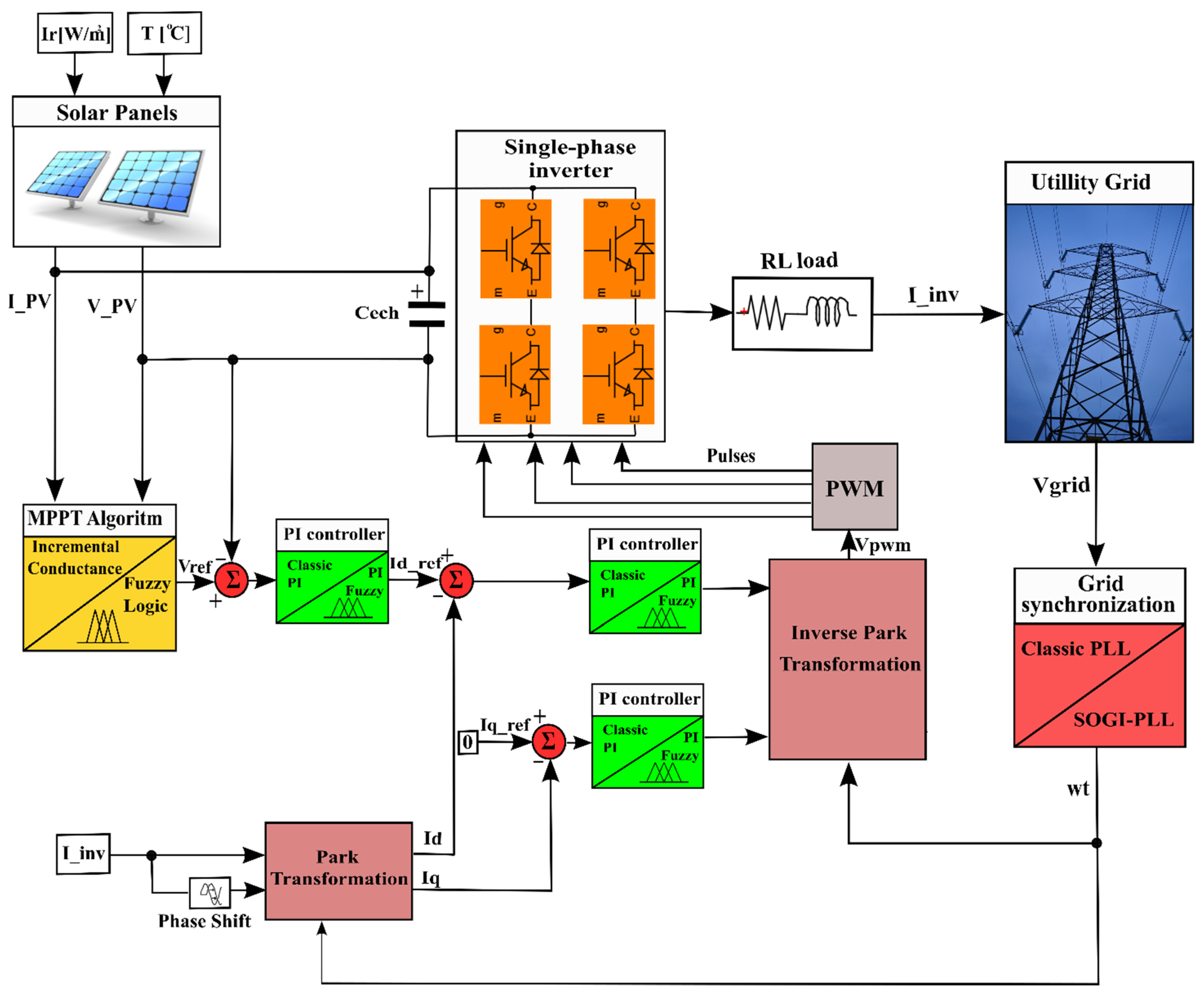
The proposed grid-connected PV inverter system setup contains a control system, a solar panel, a single-phase inverter and a load. The control system has several submodules, including MPPT and current-control logic functions, Park and Inverse Park transforms, grid synchronization, and pulse width modulated (PWM) signal generator [14]. The block diagram of the PV system for both approaches investigated is presented in Figure 1 [14].

Solar panel blocks have two inputs: irradiance value and temperature. The output goes into the MPPT block (InC or fuzzy logic), and its output provides a voltage reference for the inverter. Continuously, the signal obtained connects to the PI controller (classic or fuzzy). Finally, the latter gives the current in an adjusted form. This current, namely Id_ref, is the reference for the d-axis of the Park transformation, responsible for controlling the active power of the system.

Additionally, Park transformation generates Id and Iq (feedback current) from the inverter’s current I_inv. Feedback currents Id and Iq have to be subtracted from the reference currents Id_ref and Iq_ref. One of the reference currents, Iq_ref, is set to zero to avoid reactive power in a photovoltaic system. The obtained signals are fed into the PI controllers, then signals are amplified and integrated within the signal error to fulfill the equality conditions with the reference currents. The control currents obtained are sent to the inverse Park transformation and later modeled by the PWM generator. Henceforward, the generator’s output sends the command pulses to the inverter [14].

The inverter feeds current into the grid via an RL interconnection load, including the effects of the utility source impedance. Finally, a phase-loop (Classic PLL or SOGI-PLL) synchronizes the current injected by the inverter with the grid voltage. The sinusoidal current injected by the inverter is synchronized in phase and frequency with the grid’s voltage. In this way, the inverter is current-mode controlled to obtain the maximum useful power and deliver it to the grid [14].

2.1. Inverter Design

The topology of the single-phase inverter is shown in Figure 2. It connects mainly a DC link, power stage (inverter IGBT), and filters. The DC link consists of two 10 mF capacitors connected in series that links the DC power to the inverter system. Its high capacitance helps stabilize the input voltage for the invertor. The equivalent input capacitor can be determined with the following equation [14]:

$$C_{ech}=\frac{S}{2{\omega }_g{V}_{DC}\Delta V_{DC}}$$

(1)

where S is the apparent power, ω_g is the grid frequency, V_DC is the nominal input voltage and ΔV_DC is the input voltage ripple [14]. The inverter is connected to the grid through an RL load, made of a filter inductor of 2 mH and a resistor of 20 mΩ. The filter inductor reduces the high-frequency harmonic components injected into the grid system. The PWM logic signals G1, G2, G3, and G4 for the inverter switches are rendered by the PWM generator based on both inverter output parameters and the strategy of the control algorithm [14].

The transistors of bridge diagonals are controlled simultaneously. In this way, PWM control is used with bipolar voltage to switch on these transistors. Thus, when the pair IGBT1 and IGBT4 are commanded for opening, the IGBT2 and IGBT3 are locked and vice versa. Consequently, the four power transistors require two additional PWM width-modulated control signals with dead time [14].

2.2. Clarke and Park Transformations

2.2.1. Clarke Transformation

The Clarke mathematical transformation, also called the alpha–beta transformation, transposes a three-phase system into an orthogonal system [15]. The transformation is defined mathematically by the relation (2):

$$\left[\begin{array}{c}{v}_{\mathsf{\alpha }}\\ v_{\mathsf{\beta }}\end{array}\right]=\left[\begin{array}{ccc}\frac{2}{3}& \frac{-1}{3}& \frac{-1}{3}\\ 0& \frac{1}{\sqrt{3}}& \frac{-1}{\sqrt{3}}\end{array}\right]·\left[\begin{array}{c}{v}_a\\ v_b\\ v_c\end{array}\right]$$

(2)

where the inverse transformation is defined by the statement (3):

$$\left[\begin{array}{c}{v}_a\\ v_b\\ v_c\end{array}\right]=\left[\begin{array}{cc}1& 0\\ \frac{-1}{2}& \frac{\sqrt{3}}{2}\\ \frac{-1}{2}& \frac{-\sqrt{3}}{2}\end{array}\right]·\left[\begin{array}{c}{v}_{\alpha }\\ v_{\beta }\end{array}\right]$$

(3)

Considering that the sinusoidal variables va, vb, and vc describe a balanced three-phase system, they will have the expressions [15]:

$$v_a=V_a·\sin \omega t$$

(4)

$$v_b=V_b·\sin (\omega t-\frac{2\pi }{3})$$

(5)

$$v_c=V_c·\sin (\omega t-\frac{4\pi }{3})$$

(6)

$$V_a=V_b=V_c$$

(7)

Under these conditions, by substituting (4)–(7) in Equation (2), the following relations can be expressed [15]:

$$v_{\alpha }=v_a=V_a\sin \omega t$$

(8)

$$v_{\beta }=V_a·\sin \left(\omega t-\frac{\pi }{2}\right)=-V_a·\cos \omega t$$

(9)

In a single-phase system, there are only one of the three sinusoidal variables. Next, this unique variable is assumed to be va, and is part of a permanently balanced three-phase imaginary system. Because the alpha–beta transformation is specific to three-phase systems, Equations (8) and (9), under the assumed conditions, describe a way to obtain the two orthogonal variables vα and v_β in the case of a single-phase system [15].

2.2.2. Park Transformation

The two orthogonal variables v_α and v_β obtained with the Clarke transformation are provided to a system of rotating vectors, v_d and v_q, which rotate at an angle θ. The Park transformation is defined by the following equation considering v_α and v_β the orthogonal variables resulting from the application of the Clarke transformation [15]:

$$\left[\begin{array}{c}{v}_d\\ v_q\end{array}\right]=\left[\begin{array}{cc}\cos \theta & \sin \theta \\ -\sin \theta & \cos \theta \end{array}\right]·\left[\begin{array}{c}{v}_{\alpha }\\ v_{\beta }\end{array}\right]$$

(10)

and the inverse transformation is:

$$\left[\begin{array}{c}{v}_{\alpha }\\ v_{\beta }\end{array}\right]=\left[\begin{array}{cc}\cos \theta & -\sin \theta \\ \sin \theta & \cos \theta \end{array}\right]·\left[\begin{array}{c}{v}_d\\ v_q\end{array}\right]$$

(11)

Considering the variables v_α and v_β concerning expressions obtained from (8) and (9), we obtain the variables v^d and v^q [15]:

$$v_d=V_a·\sin \omega t·\cos \theta -V_a·\cos \omega t·\sin \theta$$

(12)

$$v_q=-V_a·\sin \omega t·\sin \theta -V_a·\cos \omega t·\cos \theta$$

(13)

If the angle θ varies in time with the same velocity as the argument of the sinusoidal component of the phase from the three-phase system, namely ωt, and if we consider the substitution θ = ωt, we obtain [15]:

$$v_d=V_a·\left(\sin \omega t·\cos \omega t-\cos \omega t·\sin \omega t\right)=0$$

(14)

$$v_q=-V_a·({\sin }^2\omega t+{\cos }^2\omega t)=-V_a$$

(15)

From Equations (14) and (15), resulting from the previously assumed conditions, the variables v_d and v_q obtained by the Park transformation are constant values in time for a perfectly balanced three-phase system. The variable v_d becomes null, and the variable v_q contains the amplitude information of a phase in the single-phase system [15].

2.3. Incremental Conductance System Description

A photovoltaic array has an optimal operating point, known as the maximum power point, which varies depending on the cell temperature and the level of irradiation. The usual approach to maximize the power absorbed by solar panels under different atmospheric conditions is to use a maximum power point tracking (MPPT) method. This technique provides a voltage reference for the inverter that interfaces the solar panel with the grid. The incremental conductance method is widely used in photovoltaic systems because it tracks changing conditions faster than the perturbation and observation (P&O) method. However, it is computationally more complex for the controller. [16]

In the incremental conductance method, the controller measures the incremental changes in the current and voltage of the PV array to predict the effect of a change in voltage. This method uses the PV array’s incremental conductance (dI/dV) to calculate the sign change in the power variation versus voltage variation (dP/dV). Knowing that the power is expressed concerning current, when (dI/dV) is equal to −I/V or both dV and dI are null, the algorithm knows that the maximum power point is reached. Thus, it ends and returns the corresponding value of the operating voltage for MPP [16]. Alternatively, when the variations are different (dI/dV) from −I/V, respectively, dV is null, and dI is positive or negative but not zero, the approach is the following: before returning to the voltage value of the MPP, the operating voltage is either increased or decreased. Figure 3 represents the flow chart of the incremental conductance method, and it offers a better understanding of the process [16].

In Figure 4, we have the circuit in the Matlab/Simulink implementation for the incremental conductance algorithm.

Both solar panel current and voltage are measured and fitted as input signals for the algorithm. The difference between each signal is obtained by delaying the corresponding input signals (I and V) and subtracting them from the values of the signals sampled and obtained from Vdelta and Idelta signals [17]. The memory block was set to zero for the initial calculation. The block Switch 3 compares the value of Vdelta with zero and divides the algorithm into the top part and the bottom part. The top corresponds to the case when the value of Vdelta is zero. The following comparison is for current values. If the Idelta variation is zero, the adjustment signal passes without any change, and the maximum power point is found. If Idelta is positive, the adjustment signal is incremented by 0.01, and the negative adjustment signal is incremented. This calculation is a linear approximation of the current-voltage slope characteristic near the MPP. The bottom part corresponds to the case when there is a variation of the voltage signal, which means that Vdelta can be any value minus the zero value that has already been calculated. When these conditions are satisfied, the MPPT has been found, and the system stops oscillating [17].

If the value ∆I/∆V = −I/V is different from zero, we must find the signal by comparing it with zero. If the result is positive, it means that the operating point is situated to the left of the maximum power point, making it necessary to increase the filling factor. This is accomplished by adding the value 0.01 to the input adjustment signal. If ∆I/∆V + I/V is negative, we do the opposite. Once the maximum power point is found, the adjustment signal is not disturbed until a new change in voltage or current is detected.

The output signal is a value between 0 and 1 controlled by the saturation block corresponding to the variation of the filling factor between 0 and 100% [17].

Then the obtained signal goes to the PI controller, giving the current in regulated form. The equation for time-domain PI controller is shown below [18]:

$$u\left(t\right)=K_p e\left(t\right)+K_i{{\displaystyle \int }}_0^{t}e\left(t\right)dt$$

(16)

The combination of proportional and integral factors is important not only to increase the speed of the response but also to eliminate the steady-state error. Here K_p is the proportional gain and K_i is the integral gain of the controller. Error signal is e(t). The signal obtained from the inverse Park transformation is fed to the PWM generator to generate a switching signal for the inverter [18].

In Figure 5, we have the PLL circuit (implemented in Simulink) for synchronization with the grid. The synchronous frame (dq) PLL converts the oscillating grid voltage and its emulated orthogonal component (αβ) to DC quantities (dq) using αβ-dq transform. Then a proportional integral controller can be used to regulate either Id or Iq to be zero so that the phase of the d or q component can be locked [19].

The PLL synchronization loop also can provide sufficient phase information to the controller to generate reactive reference current. So it allows the inverter to have the ability to control the flow of reactive power [19].

2.4. Fuzzy Logic System Description

2.4.1. Fuzzy Logic MPPT

The fuzzy logic method is widely used in PV systems because can track changing conditions more rapidly than the perturb and observe or incremental conductance algorithm. The flow chart of the fuzzy MPPT method is illustrated in Figure 6. The main elements that construct an FLC system are the fuzzifier unit at the input terminal, the inference engine with rule base, and defuzzifier at the output terminal [20].

The input parameters to the FLC are the voltage (Vpv) and current (Ipv) supplied by the solar panel. The output is represented by the inverter reference voltage (Vmppt). Based on the input signals in the MPPT block, the power is calculated, which is one of the input parameters of the fuzzy logic controller. To determine the second input of the block, namely the voltage variation (∆V), we need the current value of the voltage and its previous value. This requires the use of a delay block [21].

The next two equations give the fuzzy logic controller inputs:

$$Ppv=\mathrm{I}\_\mathrm{panel}\times \mathrm{V}\_\mathrm{panel},$$

(17)

$$\Delta Vpv=V\left(k\right)-V\left(k-1\right)$$

(18)

Figure 7 shows the implementation of the MPPT algorithm with fuzzy logic using the components provided by the Simulink (Figure 7a) and the fuzzy designer functions [22].

To implement the MPPT algorithm, the fuzzy logic designer function from Figure 7b is used. The fuzzy inference technique used is Mamdani’s approach, which is based on the max-min composition. The fuzzy database includes 49 rules expressed in terms: “If...Then” presented in

Table 1. The rule base used by the fuzzy logic controller.

	ΔVpv	NB	NM	NS	ZE	PS	PM	PB
Ppv
NB		NB	NB	NM	NM	NS	NS	ZE
NM		NB	NM	NM	NS	NS	ZE	PS
NS		NM	NM	NS	NS	ZE	PS	PS
ZE		NM	NS	NS	ZE	PS	PS	PM
PS		NS	NS	ZE	PS	PS	PM	PM
PM		NS	ZE	PS	PS	PM	PM	PB
PB		ZE	PS	PS	PM	PM	PB	PB

. Fuzzy block output (Vmppt) will be determined based on this table, and the composition of the rules will be as follows: the maximum power is reached at the output of the solar panel [22].

For example, we take a given control rule from Table 1; if Ppv is PB and ΔVpv is ZE, then Vmpp is PM. This implies that if the operating point is far from the point (MPP) to the right and the voltage change is zero, the controller should decrease the operating ratio to reach MPP [22].

Figure 7c,d show the membership functions of the input variables ∆Vpv and Ppv and Figure 7e of the output variable Vmppt, each having seven fuzzy subsets [22].

The input variables ∆Vpv and Ppv are normalized to correspond to the ranges [−1, 1] and [0, 150], and the output variable Vmppt has values in the range [34, 35] [22].

Any input value that does not correspond to the range is perceived as too high and causes signal errors. For convenience, triangular and trapezoidal membership functions are used, through which the fuzzy controller allows a rapid minimization of signal errors, ameliorating the system’s transient response [23].

2.4.2. Improvement of Control Loop with Fuzzy PI Controllers

In order to control the single-phase inverter, the control loop based on fuzzy logic was implemented. In the InC system, the control of the inverter was based on PI controllers. A detailed analysis of that system discovered some inefficiency aspects, namely a fairly pronounced transient regime in the output signals [23]. This was largely due to the PI controllers and the MPPT incremental conductance algorithm. That is why the classic PI controllers have been substituted by PI controllers based on fuzzy logic, these being more practical and efficient [24].

In the first step, the fuzzy inference system (FIS) is configured to generate a linear control interface from the E (error) and CE (error change) inputs to the output. The design of the fuzzy inference system is based on the following hypothesis [24]: The Mamdani inference method is used; an algebraic product is used for AND operation; inputs are normalized in the range [−10, 10]; the membership functions corresponding to the inputs are triangular; the output is defined in the range [−20, 20] of singleton type and is determined by the sum of the peak positions corresponding to the input sets; center of gravity (CGG) method is used for defuzzification [25].

The fuzzy logic designer function from Figure 8a is based on the above premise. The rule base includes nine rules defined in terms: “If...Then”, using the logical AND operator [25].

Figure 8b shows the membership functions of the input variables E and CE, each with three fuzzy subsets. These subsets are expressed in linguistic terms such as NEG—Negative, ZERO, and POZ—Positive. The membership function in Figure 8c corresponding to the output variable is of singleton type. It is formulated by the following linguistic terms: LargeNeg—Large Negative, SmallNeg—Small Negative, ZERO, SmallPoz—Small Positive, and LargePoz—Large Positive [25]:

To implement PI controllers based on fuzzy logic, we recalculate the gains kp, ki, corresponding to the conventional PI controllers in the incremental conductance system. The gains of the regulator, PI in the voltage loop were determined by the trial-and-error technique, establishing the values kp = −5 and ki = −30.

To calculate the PI regulator gains corresponding to the current loop, a constant time, τ_i, of 50 μs, a load inductance of 200 μH, and a load resistance of 20 mΩ are chosen.

The inductance value is sufficient because the work implies modeling a low-power photovoltaic system. Using Formulas (19) and (20), the gains kp and ki can be calculated as follows [25]:

$$k_p=\frac{L}{{\tau }_i}=\frac{200·{10}^{-6}}{50·{10}^{-6}}=4 ,$$

(19)

$$k_i=\frac{R+r_{on}}{{\tau }_i}=\frac{20·{10}^{-3}}{50·{10}^{-6}}=400,$$

(20)

To design the Fuzzy PI controller in Simulink, we need the scaling factors GE (error gain) and GCE (error change gains) for the fuzzy inputs and the output GCU (output gain). The scaling factors are calculated based on the gains kp, ki, assuming the maximum reference step 1, and therefore, the maximum error E is 1. Since the input range of the error E is [−10, 10], the error gain GE = 10 is chosen, and the other scaling factors are calculated with the following formulas [25]:

$$GCE=GE·\left(\frac{kp-\sqrt{k{p}^2}}{2·ki}\right) ,$$

(21)

$$GCU=\frac{ki}{GE},$$

(22)

After calculating the first PI fuzzy controller corresponding to the voltage control loop, the following values are obtained for the scaling factors: GE = 10, GCE = 1.66 and GCU = −3.The scaling factors corresponding to the PI Fuzzy controllers for current control were obtained with the same formulas and values GE = 10, GCE = 0, GCU = 40. In Figure 9 we have the Simulink implementation of the PI Fuzzy controllers for the voltage control loop and the current control loop. Parameters used for design this Simulink model are presented in

Table 2. Main features of the solar panel.

Voc [V]	Vmp [V]		Isc [A]	Imp [A]	Pmax [W]
21.7	17.3		4.72	4.35	75

[25].

2.4.3. Grid Synchronization SOGI-PLL

Given its advantages and wide practical use, SOGI-based PLL circuits will be used in the simulation model. The SOGI-based PLL is a highly efficient way of synchronizing PV inverter systems in a single phase, easy to design and implement. In addition, the SOGI-based PLL can operate almost like a non-delay filter with a required bandwidth [26]. In Figure 10, we have the Simulink implementation of the SOGI-PLL. Second-Order Generalized Integrator (SOGI) generates quadrature signals (QSG). The quadrature components are described by the following equation [26]:

$$v_{\alpha \beta }=\left[\begin{array}{c}{v}_{\alpha }\\ v_{\beta }\end{array}\right]=V\left[\begin{array}{c}\sin \theta \\ -\cos \theta \end{array}\right]$$

(23)

The quadrature signals are given as entries in the Park transform block. These components transform the stationary reference frame into the rotating reference frame. The PI regulator behaves as a low-pass filter to remove high-frequency components. The parameters of the PI controller are critical because changing any of them will result in the loss of system synchronism [27].

2.4.4. Simulation of the Whole System in Matlab/Simulink with Fuzzy Logic and InC

Figure 11 presents the whole PV system in Matlab/Simulink for both approaches investigated with fuzzy logic and InC. The PV array is formed by connecting two 75 W panels in series. The main features of this panel are shown in Table 2. The PV output parameters vary at different solar irradiation and temperature levels.

Using the power block in Figure 11, the active and reactive power will be measured. The active power is of interest and will be inserted into the grid. The reactive power is canceled with the Iq component, whose prescription reference is null. To calculate active power (Pout) and the reactive power (Q) in the power block using the formulas below [28]:

$$P=\frac{\left|Vinv\right|}{\sqrt{2}}·\frac{\left|Iinv\right|}{\sqrt{2}}·\cos \phi$$

(24)

$$Q=\frac{\left|Vinv\right|}{\sqrt{2}}·\frac{\left|Iinv\right|}{\sqrt{2}}·\sin \phi$$

(25)

where φ is the phase shift between current and voltage:

$$\phi =<V-<I$$

(26)

The next section presents the results of the simulations of the whole PV system with fuzzy logic and InC, and a comparison between these methods. The Vpanel and Ipanel are used to calculate the solar power (Pin), and Vinv and Iinv are used to calculate active power (Pout). The ratio between Pout/Pin will show the effectiveness of the power conversion in the PV system for both approaches.

3. Simulation Results

The following figures depict the simulation results for the system shown in Figure 11. All simulations from both approaches are executed only at a fixed temperature of 25 °C, and step variation with solar irradiation of 1000 W/m², 500 W/m². Figure 12 shows the irradiance variation to produce the partial shading effect.

3.1. Incremental Conductance System Results

The next figures (Figure 13, Figure 14 and Figure 15) illustrate the system’s simulation results modeled with the InC method.

Figure 13 shows the voltage, current, and power extracted from the solar panel. It can be observed that the parameters which fluctuate the most concerning irradiation variation are the current and the power. On the other hand, the voltage remains nearly constant.

Figure 14 displays the output inverter current, inverter voltage, and grid voltage. It can be observed in the following image (Figure 14) that the output current is proportional to the irradiance.

Figure 15 illustrates the solar panel power (Pin), which ranges from 148.8 W to 152.3 W, and the output power (Pout-IC) ranges from 96 W to 137.3 W at 1000 W/m² irradiance. Therefore, the system based on InC has a low efficiency of around 80%.

3.2. Fuzzy Logic System Results

In this subsection, we continue with the FLC algorithms results. Therefore, Figure 16 presents an output characteristic of the solar panel showing the voltage, current, and power, the latter two varying concerning the irradiance.

Improving characteristics of the solar panel by adding fuzzy logic leads to an increase in the efficiency of the photovoltaic system. Thus, the DC power can be stored almost entirely by the inverter and converted into AC power.

The previous image (Figure 17) presents the output characteristics of the inverter (I_inv, V_grid, V_inv). The current tracks the power signal, respecting the irradiance’s change one more time.

In the first stage, a comparison was made between the voltage (V_PV), current (I_PV), and power (Pin) characteristics obtained at the output of the solar panel, corresponding to the two methods; this being presented in Figure 13 and Figure 16. Taking the characteristics one by one and comparing them, we can see the difference between the two approaches, which are not negligible. The InC output solar panels characteristic has a pronounced transient regime, significant oscillations, and the maximum voltage is not reached, whereas if we analyze the FLC solar panel characteristics, we notice a fast response, the transient regime is almost non-existent, and the maximum voltage is reached without problems.

Making the same comparative analysis between the output characteristics of the inverter, we again notice that the FLC method improves the regime transient, rapid response, elimination of oscillations, and overgrowths corresponding to the InC system.

The following figure (Figure 18) illustrates the power-transfer performance. The output power of the solar panel (Pin) is between 149.8 W and 150.2 W, and the active power (Pout-FLC) is between 149.5 and 149.9 W at 1000 W/m² irradiance. Therefore, the system based on fuzzy logic has an efficiency of around 99.80%.

Figure 19 shows the output voltage of the fuzzy MPPT controller. At the initial time, when the maximum irradiance value is 1000 W/m²; the Vmppt voltage is 34.8 V. If the irradiance goes down to 500 W/m², there is a slight drop in voltage to 34.5 V, which would correspond to the new maximum power point. Therefore, it can be seen that the inverter reference voltage (Vmppt) is constant at constant irradiance and has very small variations with irradiance changes; this demonstrates that the fuzzy-based MPPT algorithm provides high accuracy in determining the maximum power point.

The grid synchronization signal (wt) from the SOGI-PLL loop output is shown in Figure 20. The synchronization signal will have the peak amplitude at 2π, as seen in the picture below.

Figure 21 shows an overlap of power characteristics at the output of the inverter (Power Out), obtained after simulating the PV system based on the incremental conductance MPPT algorithm (Pout-IC) and the system based on fuzzy logic (Pout-FLC). The green characteristic represents the power obtained at the inverter output within the InC system. The orange characteristic represents the power obtained at the inverter output within the FLC system. The green feature has a high transient regime (about 10% of the simulation time), and after that, the feature shows quite pronounced oscillations and overgrowth when changing the irradiance. This involves power losses at the inverter output, which shows that the system implemented with incremental conductance is less efficient. The orange characteristic shows a prompt response, the transient regime being almost eliminated; it does not show oscillations and overgrowths at the sudden irradiance change. This proves that the system implemented with fuzzy logic shows potential and is more efficient.

4. Conclusions

In this article, a comparative study highlights the difference between the two techniques of controlling a low-power PV system. One technique used the fuzzy logic MPPT and fuzzy PI controllers in the control loop and SOGI-PLL in the grid synchronization. The other was based on incremental conductance MPPT, classic PI controllers, and classic PLL grid synchronization. Theoretically and through simulations in the Matlab/Simulink software, the perspectives were established and contrasted based on the strengths and disadvantages of the two techniques. Based on theoretical analyses and results of the simulations, we can draw the following conclusions:

• Intelligent techniques based on FLC and ANN are very sensitive and consume significant computational resources.
• The AI method based on fuzzy logic presents advantages over the InC method. These advantages are mainly due to the fuzzy MPPT controller, which offers a better extraction of the maximum power from PV modules.
• The fuzzy PI regulators help improve the control loop of the single-phase inverter and reduce the transient response comparatively with classic PI.
• The transient regime represents 1.5% from simulation time, allowing the system to reach fast (0.03 s) in tracking the maximum power. Moreover, the proposed model converts solar energy with a performance of 99.8%. On other existing research [29,30], several energy conversion performance results are presented, where the best fuzzy logic technique reported a 99.19% conversion efficiency with a 1.7 % transient regime of the simulation time.
• The SOGI-PLL grid synchronization mechanism with the utility grid is more powerful with a higher stability margin than the classic PLL.

Consequently, the FLC technique proves to be fast, flexible, and robust. These benefits represent key features for spontaneous change situations in environmental conditions. Moreover, fuzzy logic helps the inverter convert over 99% of the power generated by the photovoltaic panels, while the incremental conductance algorithm converts around 80%. In conclusion, energy losses in the proposed PV system are more significant for InC approaches when compared with the FLC method.