Abstract
Most photographs are low dynamic range (LDR) images that might not perfectly describe the scene as perceived by humans due to the difference in dynamic ranges between photography and natural scenes. High dynamic range (HDR) images have been used widely to depict the natural scene as accurately as possible. Even though HDR images can be generated by an exposure bracketing method or HDR-supported cameras, most photos are still taken as LDR due to annoyance. In this paper, we propose a method that can produce an HDR image from a single arbitrary exposure LDR image. The proposed method, HSVNet, is a deep learning architecture using a Convolutional Neural Networks (CNN) based U-net. Our model uses the HSV color space that enables the network to identify saturated regions and adaptively focus on crucial components. We generated a paired LDR-HDR image dataset of diverse scenes including under/oversaturated regions for training and testing. We also show the effectiveness of our method through experiments, compared to existing methods.
1. Introduction
High dynamic range (HDR) photographs include rich color details by using higher color depths to encode a broad range of real-world luminance. Conventional color images and displays using the 8-bit depth for each color channel can only convey a limited range of color, which is called a low dynamic range (LDR), compared to the HDR. Especially when we take a picture in extremely bright scenery with some dark areas such as shadows under the sunlight or dark scenery with some bright areas such as the moon at night, the picture may partially contain very bright or dark areas. This results in missing details in over/underexposed areas of LDR images. However, creating a sound-quality HDR image with a standard camera setting is bothersome. We usually use exposure bracketing, which shoots multiple exposure images and merges them into an HDR image.
There has been active research towards developing the reconstructing process of HDR images from LDR images to be more universal. Thanks to advances in hardware technology, high-end cameras can capture 3 or 5 different exposure images at the same time and fuse them into an HDR image automatically. However, there are still a few unsolved problems: the price of specialized cameras, moving objects, and camera angle stabilization [1,2]. Many researchers have also developed software solutions to create an HDR image from a single LDR image. Inverse tone mapping (iTMO) [3] is a process that expands an LDR image to an HDR image for visualizing on a high dynamic range display. Several iTMO methods have been proposed based on mathematical models which infer color details in missing areas from LDR images [4,5,6]. However, those models have limitations that could not consider each image’s individual characteristics and relationships between channels. Recent advances in deep learning neural networks for the computer vision field enable numerous approaches to minimize these limitations. Deep Neural Networks, especially convolutional neural networks, help models to comprehend the complex nonlinearity between the input image and the target image, which is arduous for humans to detect [7,8,9,10]. However, there are existing limitations. Expanding an 8-bit LDR image to a 32-bit HDR image is still challenging because of the lost details in over/undersaturated regions and too low or high exposure images [10,11,12,13]. To solve these problems, we propose a method that lets a model find and concentrate on over/undersaturated regions. Additionally, the proposed method is able to convert the images which are captured by not only middle exposure but low or high exposure to HDR images.
In this paper, we propose a convolutional neural network architecture, HSVNet, for reconstructing an HDR image from a single-exposure LDR input image. We utilize U-net with a mask and a customized loss function. For training, we make our own paired LDR-HDR image dataset by taking multiple-exposure LDR images and fusing them into an HDR image. We also gather a paired LDR-HDR image dataset from the image source [14]. In the network, the color space of the input image, which is usually RGB (Red, Green, and Blue), is converted to HSV (Hue, Saturation, and Value) color space. We use HSV color space in this paper because the HSV color space is designed to more closely represent the human perception of color. Since each channel in the HSV space represents a perceptual attribute of color, we believe that deep neural networks can learn the ground truth more concisely. Specifically, the V channel represents the brightness which is directly related to the high dynamic range of natural lights. Additionally, the hue of color in RGB space is determined by the ratio between three channels, which can make it difficult to reconstruct them. A better estimation is expected by separating these attributes. Reconstructing HDR in RGB color space may feature a weakness such as severe local inversion artifacts on reconstructed HDR images and insufficient contrast [2,15,16]. This is partly because loss functions were simple mean-absolute error (MAE) or mean-squared error (MSE) between the predicted and target images. Therefore, we propose a customized loss function for HSV color space which allows the network to output reliable and natural color.
This paper presents the following three main contributions.
- 1
- We propose a deep learning system that can reconstruct a high-quality HDR image (32-bit) from an arbitrary single-exposed LDR image (8-bit) which may include both over- and undersaturated regions;
- 2
- We present a mask function derived from Saturation (S) and Value (V) information in HSV color space which can detect both over- and underexposed areas and suppress unnecessary information for each channel;
- 3
- We propose a customized loss function appropriate for HSV color space and choose an optimal loss function by experiments.
2. Related Works
There has been extensive research on reconstructing HDR images from LDR images, which is also known as inverse tone mapping [3]. This problem is still challenging because of the missing information on over/undersaturated regions. In this section, we summarize previous research.
2.1. Non-Learning Methods
In the early years, non-learning methods based on mostly mathematical models were proposed. Banterle et al. [3] first presented inverse tone mapping operations and utilized the Median Cut algorithm [17] to find high luminance areas and generate an expand-map from the result of density estimation of the areas. Rempel et al. [4] applied a Gaussian function to an expand map. They then used an edge stopping function to enhance the brightness of saturated areas. Kovaleski and Oliviera [5] exploited analogous steps to Rempel et al. by using an inverse tone mapping based on cross bilateral filtering. Wang et al. [6] presented a hallucination method that requires user interaction. The saturated region could be re-filled with texture information from a user-selected source region. Meylan et al. [18] applied a piece-wise linear tone scale function to expand the specular and diffuse parts in the image. The unnatural artifacts from discontinuity in the tone scale function were suppressed by adding a smoothing step. Masia et al. improved on their previous methods [19], which had the shortcoming of insufficient performance for the large oversaturated input images, by proposing a global iTMO based on a simple gamma expansion [20]. Huo et al. [21] proposed a psychological iTMO based on the HVS (Human Visual System) using the local retina response for minimizing artifacts. Sen et al. [22] proposed a patch-based approach. They generated highly related local features of the result with all LDR images directly. The alignment and merging process could be completed at the same time.
2.2. Learning Methods
In recent years, methods utilizing deep learning from input to targeting ground truth have been actively presented, due to the excellent performance on analytic training. Most of them were based on a convolutional neural network (CNN). Chen et al. [7] expanded an 8-bit LDR image to a 16-bit image by utilizing a U-net-based network with a spatial feature transform (SFT) layer. Eilertsen et al. [8] also used a U-net with gamma corrected skip connections. They proposed a masking method to find overexposed regions in images. The masks were created by the maximum value among red, green, and blue channels and used for blending an input image and a predicted image. Marnerides et al. [9] attempted to capture different levels of features in input LDR images. They proposed 3 different branches—local, dilated, and global branches. Local/global branches have a small/big receptive field for high-level features/low-level features. The dilation branch captures mid-level features. Yang et al. [23] introduced a U-net-based image correction method which reconstructs an HDR image from an LDR image first and then renders a color-corrected LDR image from the HDR domain. Khan et al. [24] suggested an end-to-end feedback network that was effective for rendering a coarse-to-fine representation. They learned the feedback network using the recurrent neural network multiple times resulting in a deeper network for better reconstruction quality. Liu et al. [10] designed a pipeline in a sequence of clipping, a non-linear mapping, and quantization for HDR images to LDR images. They then trained the CNN model to learn each reversed step of the pipeline. For loss functions, MAE, MSE, and perceptual loss from the VGG network [25] were employed. Additionally, Santos et al. [26] utilized perceptual loss. They applied the sum of MAE loss and perceptual loss as a loss function. They used a U-net architecture with masks kept updated every step. Li et al. [27] suggested the attention approach. They devised a network with two different branches, which are the attention branch and the dilation branch, for finding interdependencies between channels.
After generative adversarial networks (GAN) [28] were presented, GAN demonstrated its exceptional performance in image translation. Researchers applied the concept of GAN to inverse tone mapping since it also maps input images to target images. A GAN-based inverse tone mapping approach was first proposed by Niu et al. [11]. They suggested the model with adversarial learning to eliminate the misalignment from large motions. Moriwaki et al. [16] proposed a hybrid loss function. The proposed loss function was the sum of reconstruction loss (MAE), adversarial loss (GAN loss), and perceptual loss (VGG loss). Kim et al. [29] also applied the GAN-based framework to their three subnetworks for image reconstruction, a detail restoration, and a local contrast enhancement. Marnerides et al. [30] used a GAN-based architecture with a Gaussian distribution to transform the density of HDR pixels.
There has been some research that attempted to use the HSV color space. Ye et al. [12] applied a Hue loss function with a simple MAE. They proposed a network with two branches for overexposed and underexposed areas, respectively. Two kinds of masks, light and gray masks, were employed for training, which was calculated by the gray scale of an LDR image. Wang et al. [13] also employed an HSV loss function. They utilized saturation information for their loss function with a simple MAE. Their network predicted different exposure images from an input image and then merged all of them into an HDR image.
3. Method
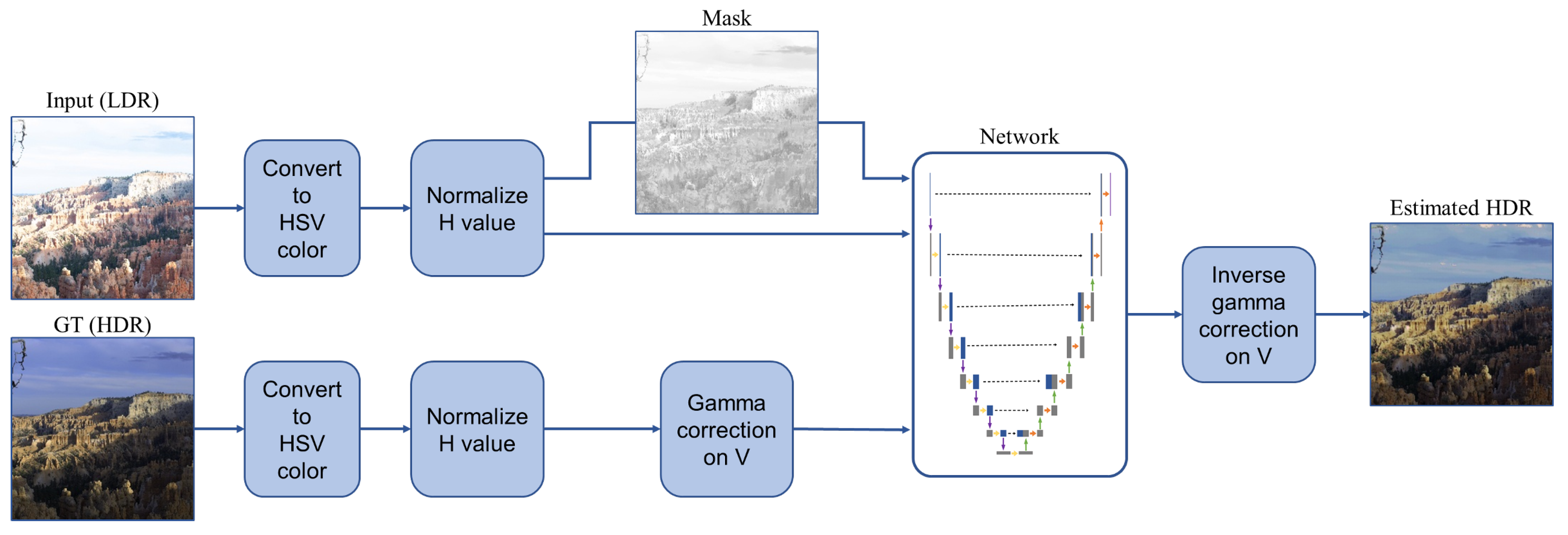
We propose a method to generate an HDR image from an LDR image with a deep learning architecture. Our proposed method first (1) pr3processes the data by converting color space into HSV, normalizing H, and a gamma correction on V channel of ground truth for the normalized range in , (2) creates a mask for each input LDR image, (3) learns the U-net based network, HSVNet, to generate an HDR image by uncovering the relationship between H, S, and V color components, and (4) postprocesses the prediction to recover the original range of V with an inverse gamma correction () on the V channel,
where H is the reconstructed HDR, i is the index of image, v is V channel, and is the network output. The overall process of our framework is shown in Figure 1. First, we convert the input and the corresponding ground truth image to HSV color. Then, we normalize all values which are out of the range and create a mask of the normalized input. We transfer the normalized input, mask, and ground truth to our network. The mask is used as a weight in a loss function. Finally, we map the values of the estimated image to the original range of the ground truth to obtain a genuine HDR predicted image.
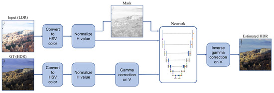
Figure 1.
Our framework first converts the color space to HSV and normalizes H values. Then it creates a mask for each input LDR image and applies a gamma correction on V of the ground truth. It finally estimates an HDR image by applying an inverse gamma correction to the result from the network.
3.1. Architecture
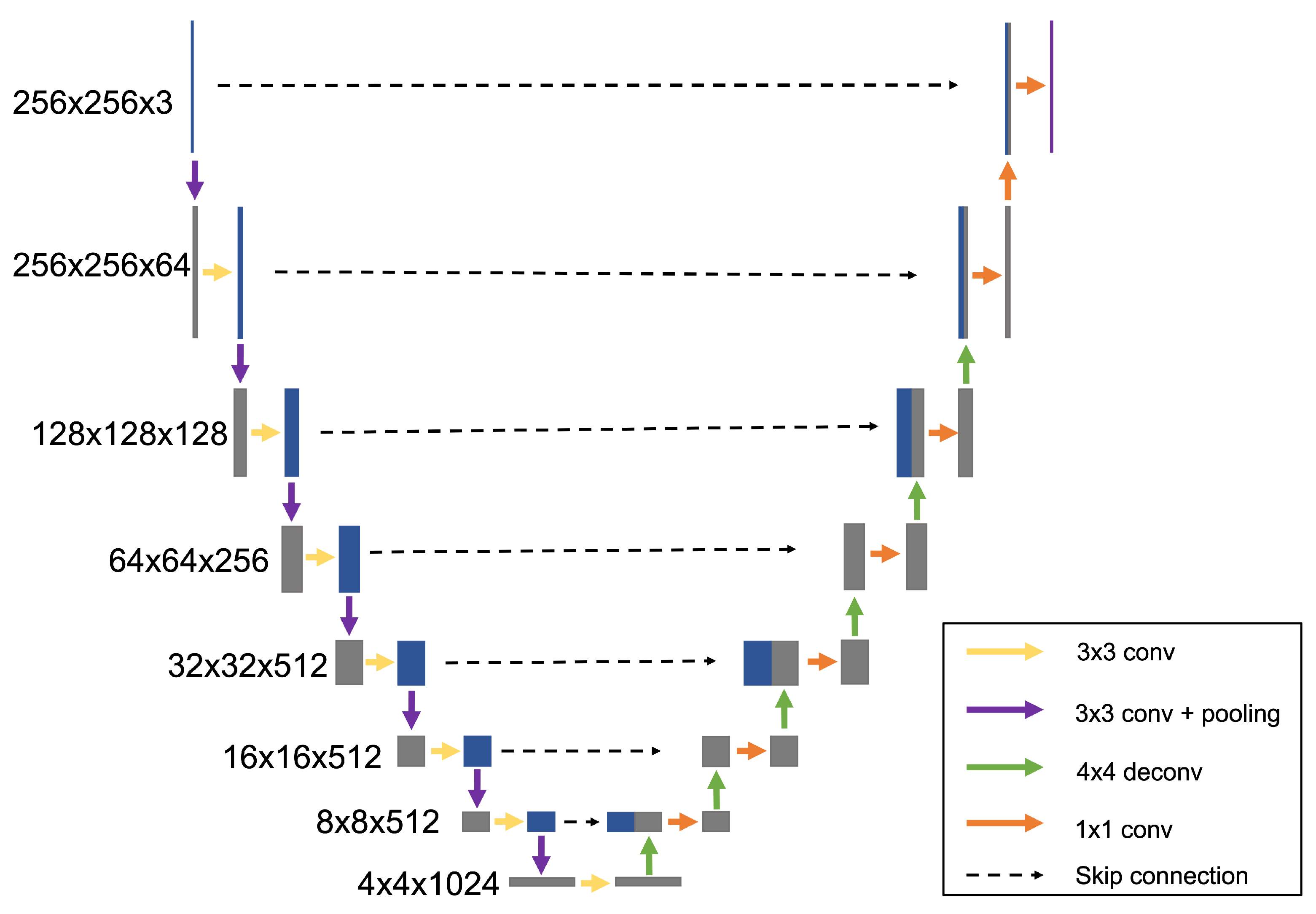
An autoencoder is a feedforward neural network that is trained to attempt to copy its input to output by reducing the input to low-dimensional data and reconstructing high-dimensional data as the output [31,32]. The autoencoder consists of an encoder part (contracting path) and a decoder (expansive path). U-net is an autoencoder with skip connections between encoder and decoder [33]. The skip connections help rebuild the high-frequency features, such as border pixels, which could be lost from the deep convolution layer [34]. We use the same concept for the reconstruction of HDR images. Our proposed network is shown in Figure 2. The proposed network is based on the well-known VGG-16 network [25].
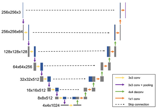
Figure 2.
Our HSVNet architecture with U-net.
In the encoder layer, the spatial feature resolution is gradually reduced by half from 256 to 4, applying convolutions with stride 1. After a bottleneck layer, the decoder reconstructs full-dimensional data from the latent data by upsampling. The decoder process is the reversed encoder process. We use deconvolution for upsampling with stride 2. There are skip connections between encoder and decoder to preserve the detailed information. Each skip connection concatenates the encoder layer and the decoder layer corresponding to the resolution. Then, the concatenated layer is downsampled with convolutions with stride 1 to reduce the number of feature channels by half. We use ReLU activation function at every layer.
3.2. Loss Function
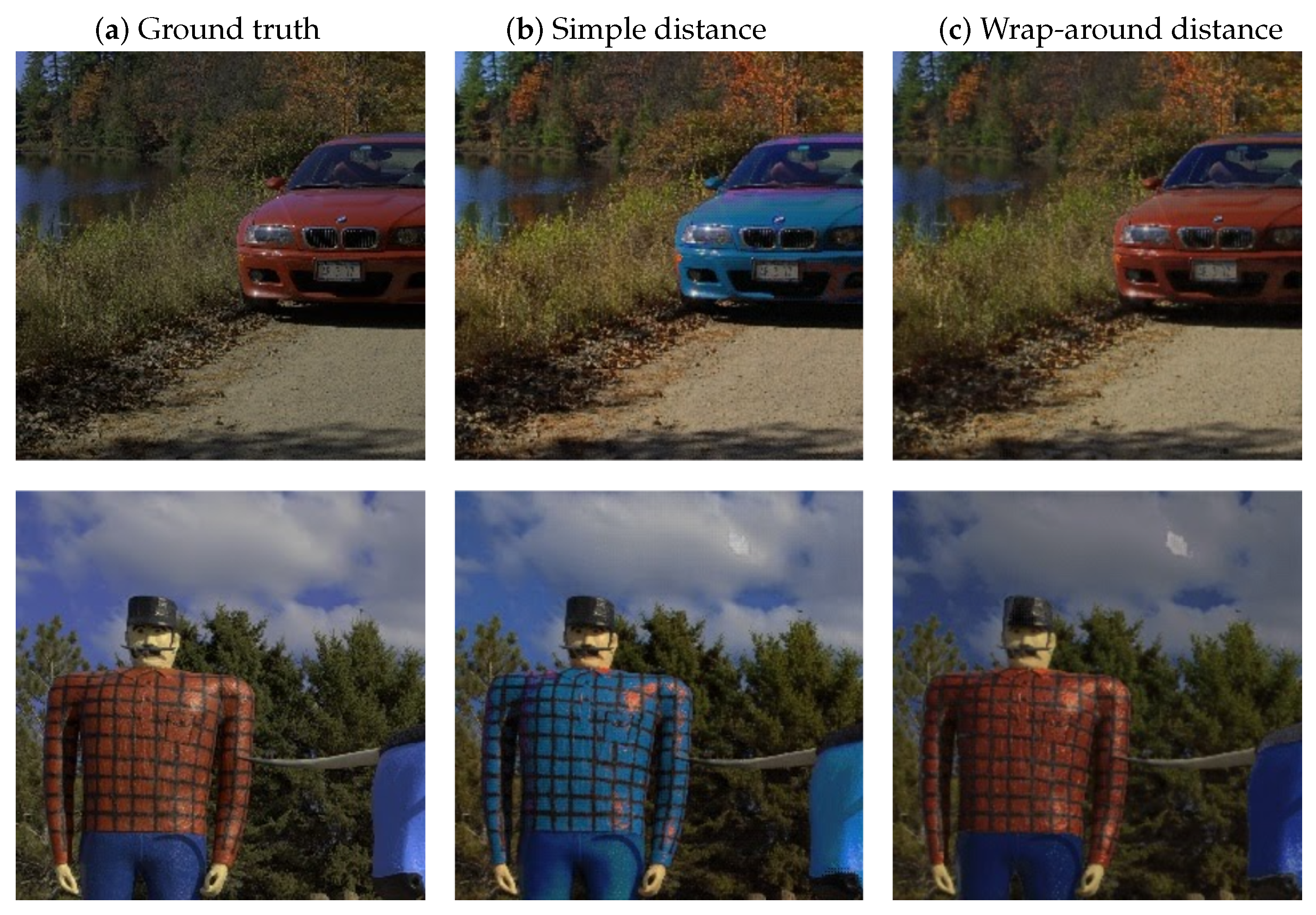
A normal Mean Absolute Error (MAE) is applied to S and V channels. Unlike Saturation and Value, Hue is angular data. When MAE is directly applied to the H channel, the model cannot predict the color around the red correctly. Even though both and indicate the same red color, MAE gives the highest penalty when predicted H is and target H is or vice versa. Therefore, the red color might converge to the average value of and . As shown in Figure 3, the predicted images with a MAE H loss may have local artifacts, e.g., the red color is predicted as blue.
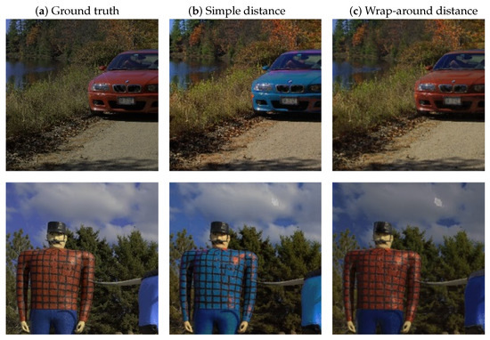
Figure 3.
Comparison of simple distance loss (MAE) to wrap-around distance loss. All HDR images are tone-mapped in this paper.
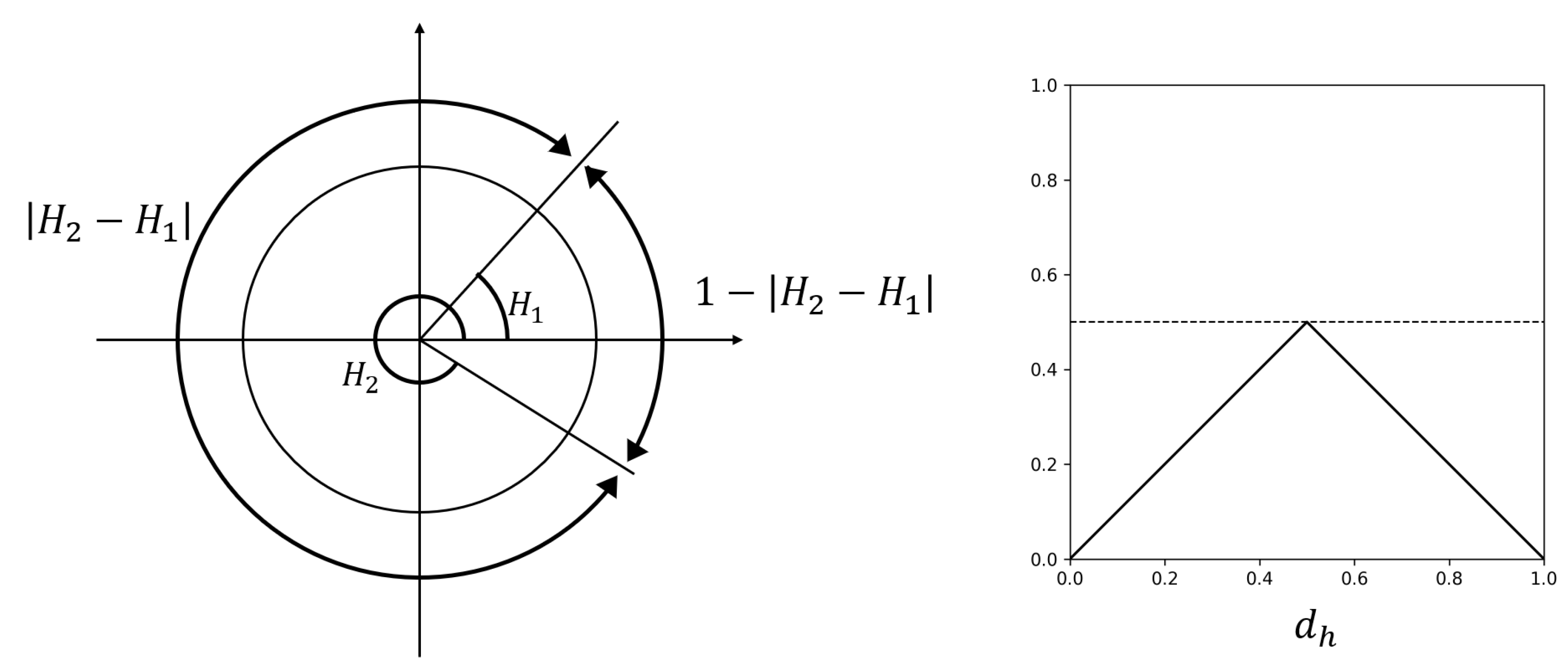
Therefore, we develop a customized loss function, , for the H channel. First, we define a simple wrap-around distance, , which is the difference between the predicted value and the target value in polar coordinates. is the angle of the shortest arc between two H values on a unit circle. As shown in Figure 4, the shortest arc angle between and can be represented as or . Since we take the shortest path, the minimum value is selected.
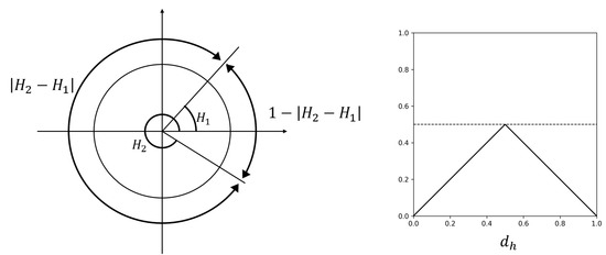
Figure 4.
(left) Wrap-around distance loss (). (right) Plot of .
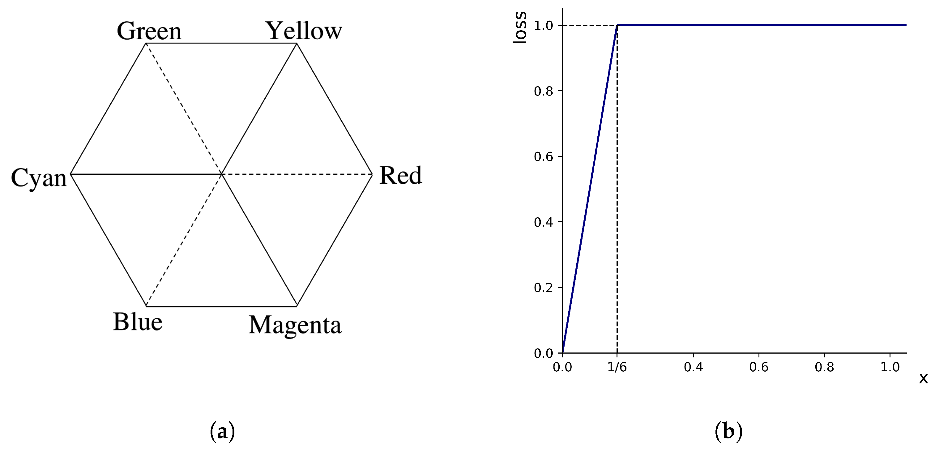
Figure 5a shows a Hue space of HSV color [35], where the angle presents the Hue. In this space, three primary colors (Red, Green, and Blue) are separated by and three secondary colors (Yellow, Cyan, and Magenta) are located from primaries. As a result, color changes largely every . For this reason, if the wrap-around distance is over 60 degrees, we assign the maximum penalty to prediction in the H loss function. In human eyes, we perceive that both cyan and green are far from red to a similar extent, even though green is closer to red in the Hue space model theoretically. Therefore, not directly applying wrap-distance to , we set the maximum penalty if is over (=) (see Figure 5b), which is a modified ramp function.
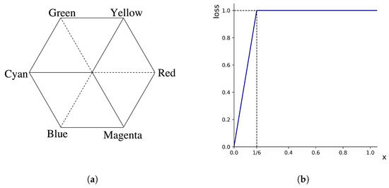
Figure 5.
(a) Hue plane in a hexagonal model. (b) Loss function for the H channel () where .
Finally, , , and are defined as
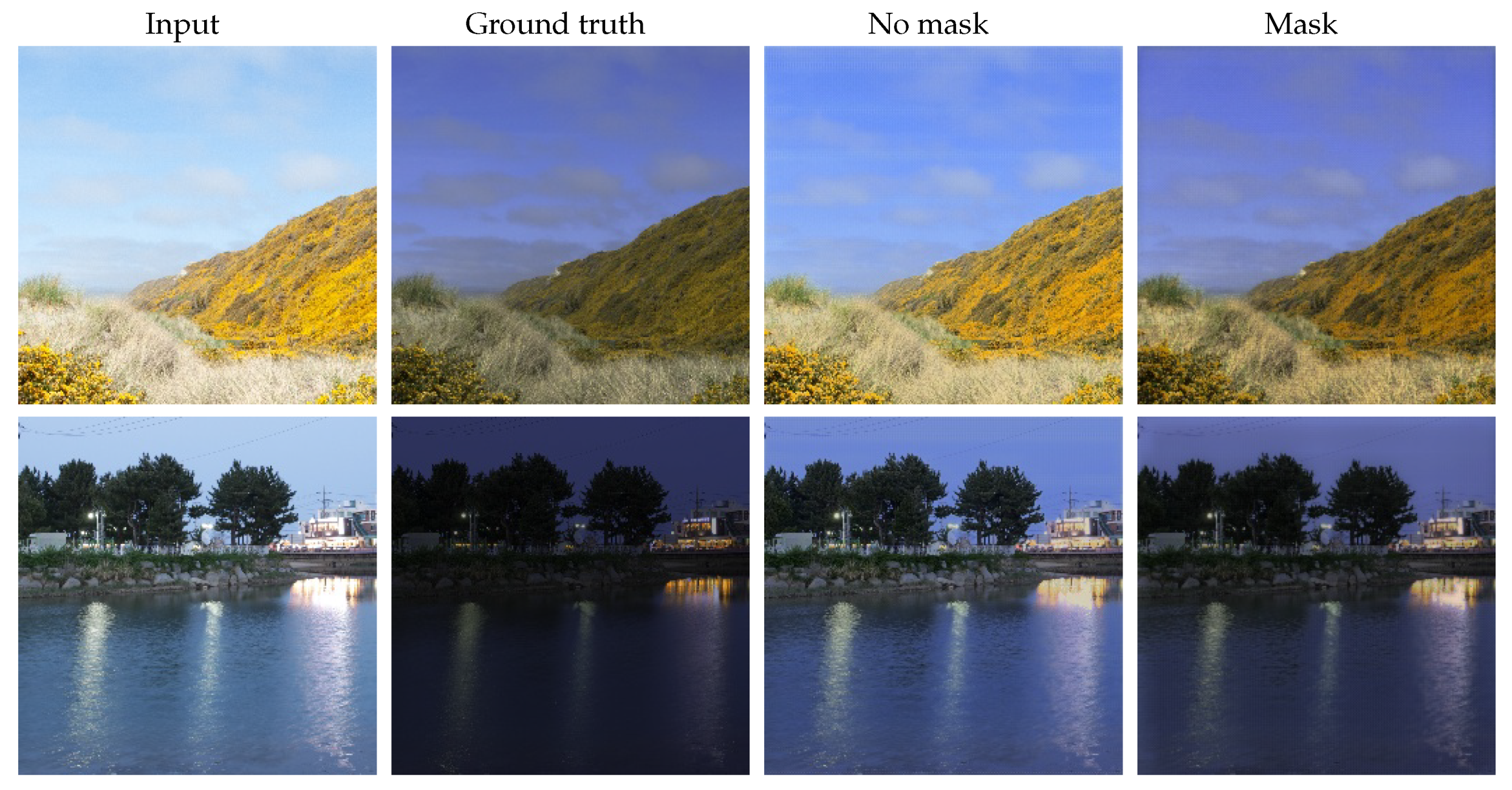
where L is a loss function with channel h, s, and v, M is a mask with channel h, s, and v, N is the number of pixels, is estimation, and y is ground truth. The total loss function L is the sum of , , and . Each mask is applied to the corresponding channel in the loss function. We recognize that there are two distinct regions where H, S, or V are differently important to the training. Therefore, the mask applied to the loss function contributes to the better quality of output by adaptively focusing on crucial regions during the training. As Figure 6 shows, the HDR images predicted with the mask are more similar to the ground truth than those without the mask. The details about the mask are discussed in Section 3.3.
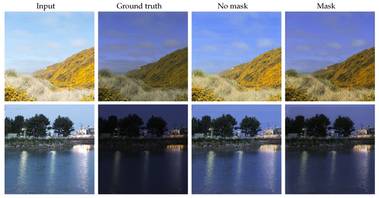
Figure 6.
Result images with and without masks.
3.3. Mask
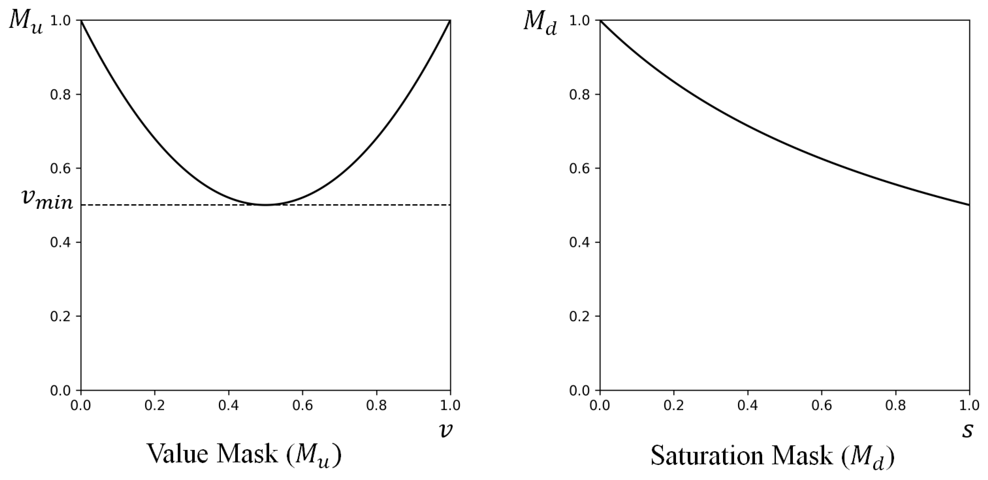
One of our main objectives is to infer color details in over/underexposed regions from the LDR image. It is essential to understand the characteristics of saturated regions in the HSV color space. H is relatively irrelevant for finding saturated pixels since the over/underexposed regions hold little information on the hue of the color. Therefore, we design a mask with S and V values that can separate saturated regions and unsaturated regions. We consider saturated areas to have the following characteristics: saturated areas have small S and high or low V (see Figure 7). We first build a saturation mask to differentiate between high saturation values and a value mask to distinguish bright and dark values. Then, we combine them into the final mask, , as shown in Equation (9):
where x is input image, and are input image’s S and V, values respectively, and c, , and are parameters for the mask. For the saturation mask , the weight is inversely proportional to the pixel’s S value, which means a pixel has a higher weight for a lower S (see Figure 8). The weight for the saturation mask is determined by adjusting c and . The weight is always 1 for the smallest S, when . Increasing c allows a more gradual descent of , where high S pixels are not sifted much. Increasing results in a more curved and steeper function. Therefore, the network focuses more on the low saturated regions with smaller c and bigger . For the value mask , a function is U-shaped between 0 and 1, where a pixel has a higher weight as V approaches two borders, 0 and 1, as shown in Figure 8. determines the weight for the value mask. The weight is 1 for the smallest and the biggest value, when and . Since lower makes the lower midpoint of , the network focuses more on bright or dark areas with lower . By the experiments on different parameters for the mask, in ranges , , and , we use , , and in this paper.
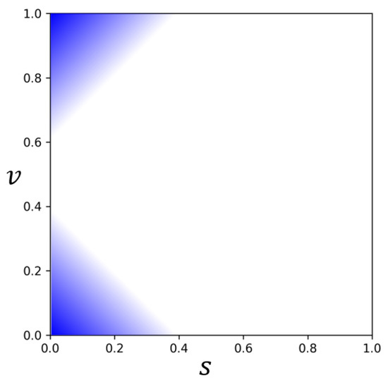
Figure 7.
Saturated region: the upper highlighted area and the lower highlighted area are considered as the oversaturated region and the undersaturated region, respectively.

Figure 8.
(left) Value mask, . (right) Saturation mask, .
Then, we use for S and V masks, , and for H, . The mask applied to our proposed loss function is as follows.
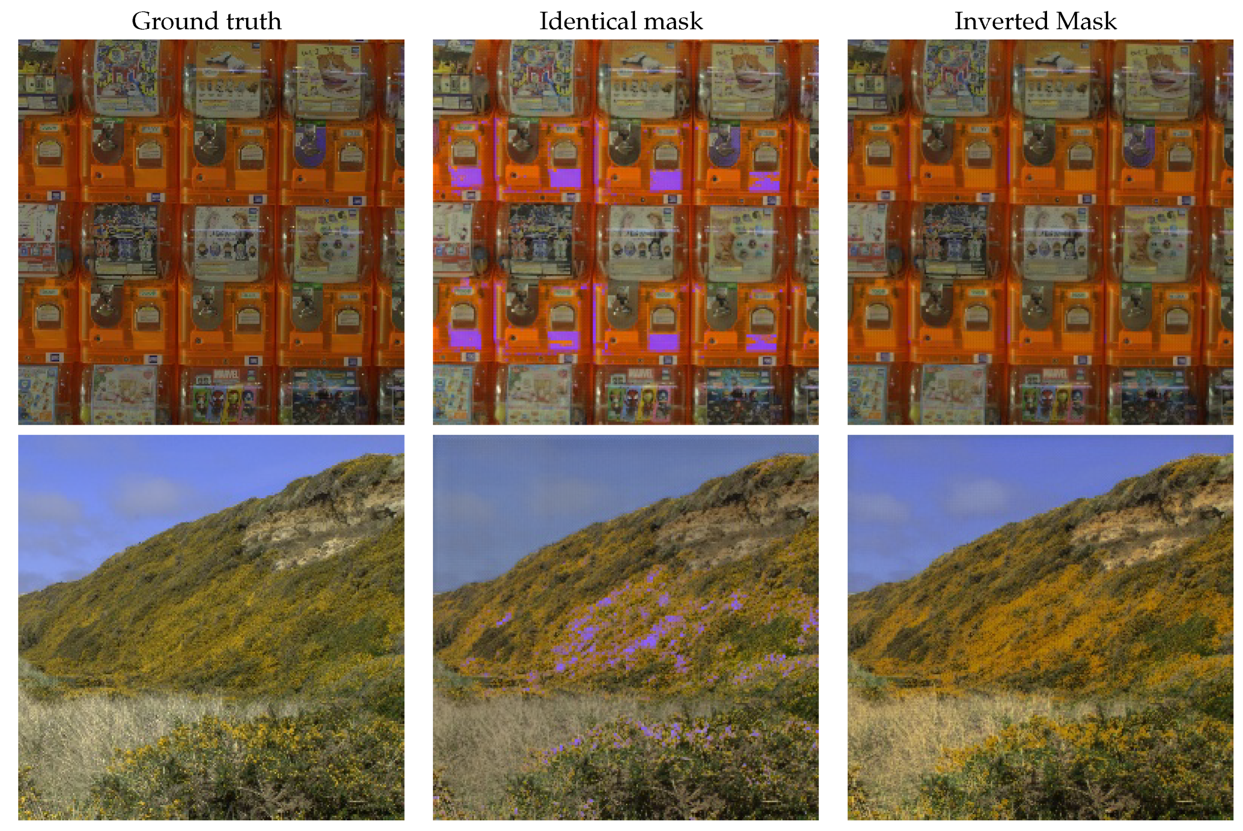
We suppress the influence of the H channel on the saturated regions when learning the network since Hue is unreliable in these regions. Therefore, we use the inverted for the mask of hue, . Figure 9 shows that the predicted HDR images could have local artifacts when the identical mask is applied to all H, S, and V channels.

Figure 9.
Result images when identical mask and inverted mask are applied to the network. Identical mask has 3 channels of for H, S, and V. Inverted mask has one channel of for H channel and two channels of for S and V channel. Artifacts can be seen in the result images of identical mask.
As shown in Figure 6, the result tends to be similar to the input image when mask is not applied. Additionally, when the same mask is applied to H, S, V, many results show artifacts (second column of Figure 9). Table 1 shows that the result with the inverted mask performs better than the result with no mask or with the identical mask.

Table 1.
Comparison of the network with no mask, the network with the identical mask, and the network with the inverted mask. The values in bold indicate the best scores for each metric.
We adopt 4 full-reference metrics to compare the performances of loss functions: L1 loss (Mean Absolute Error) [36], HDR-VDP-2.2 Q score [37], PU21-PSNR [38], and PU21-SSIM [38]. The HDR-VDP Q score suggested by Nawaria et al. is a visual metric especially for HDR images. Q score compares the quality of a test image to that of a reference image based on the human perception. The high score indicates that the test image is close enough to the reference image. PU21 is a metric for HDR images using perceptually uniform transform while overcoming the nonlinearity of PSNR and SSIM.
4. Analytical Study
To determine the optimal architecture, loss function, and masks, we tested our model in different settings including (1) the sequence of layers and (2) loss functions.
4.1. Network Variations
Our proposed network is a VGG-16-like network and we ran ablations on different layer combinations. We experimented in order to confirm the optimal network for our dataset. We stacked up more layers than VGG-16 for expanding the receptive field. We experimented with variations in the VGG-16-like network (see Figure 10): (a) a network with convolution layers always followed by a pooling layer, (b) a network with consecutive blocks, each with one non-pooling convolution layer and one convolution layer followed by a pooling layer, and (c) a network with blocks with two non-pooling convolution layers and one convolution layer, followed by a pooling layer.
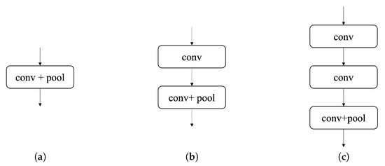
Figure 10.
Block variations of the network. (a) Convolution layer followed by a pooling layer, (b) one non-pooling convolution layer and one convolution layer followed by a pooling layer (ours), and (c) two non-pooling convolution layers and one convolution layer followed by a pooling.
The performances of the second and the third network were meaningfully better than the first one. Especially, the result of the third network is slightly better than that of the second network (see Table 2). However, the training time of the third network is much longer than the second one. The training times of network (1), (2), and (3) are 2 h 30 min, 3 h, and 4 h, respectively. Based on these results, we decided to use the second network.
Table 2.
The test results for networks (1), (2), and (3) shown in Figure 10. The values in bold indicate the best scores for each metric.
4.2. Loss Function Variations
We ran variations on different loss functions.
- 1
- Cone space distance: Since HSV color space can be represented as a cone model, the most intuitive difference between two HSV colors will be a Euclidean distance in a cone space. In this method, we convert HSV colors of H, S, and V to points in a cone space and calculate a Euclidean distance between the prediction and the target (Figure 11 left).
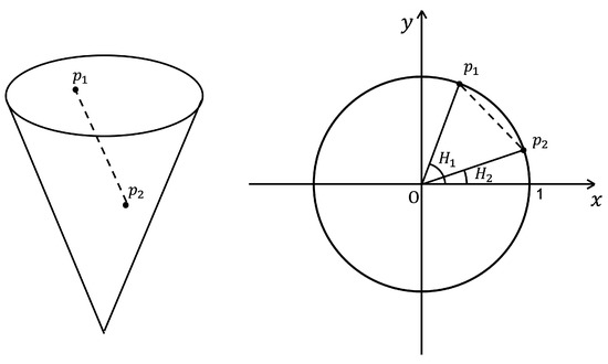 Figure 11. (left) Euclidean distance of two points on a HSV cone space. (right) Euclidean distance of two H points on a unit circle.
 - 2
- 3
- Square root of wrap-around distance (): We tried using the squared root of the wrap-around distance, , for H loss because we believe the penalty should be similar for big errors as described in Section 3.2. MAE was applied to S and V loss.
- 4
- Circle plane distance: We converted H values to the points on a unit circle in polar coordinates and calculated the Euclidean distance between two points for H loss as shown in the right image of Figure 11. This function also shows steeper slopes for smaller distances as the square root function. MAE was applied to S and V loss.
- 5
- Modified ramp: We cropped wrap-around distance and set the maximum value 1 when is over , as described in Section 3.2 (Figure 5b). MAE was applied to S and V loss. We tested the network with various degrees for the penalty threshold, and performs better than others, as shown in Table 3.
Table 3. Test results with setting the maximum penalty over different degrees in the H loss function. The H loss function with degree is . The values in bold indicate the best scores for each metric.
Table 4 presents test results for different loss functions with the same mask parameters. Although there is no single method which outperforms others in all factors, the last method of modified ramp function, , produces visually plausible results, as well as the satisfactory test results in general.
Table 4.
The test results for different loss functions: The same mask parameters are applied (, , ). The values in bold indicate the best scores for each metric.
5. Training
5.1. Dataset
A major challenge for successful development is to gather a sufficiently large paired LDR-HDR dataset which has multiple exposures of LDR images. Even though many HDR datasets are available on the web, most of them do not provide corresponding LDR images. FHDR [24] and HDRCNN [8] generated LDR images from HDR images to obtain training data. However, our goal for the dataset is to create authentic LDR images in multiple exposures paired with each HDR image. To use genuine LDR and HDR paired images, we use Fairchild database [14] which provides 7 or 9 multiple-exposure LDR images for each HDR image. We also generated our own paired dataset. We captured 504 scenes using a Canon Mark 3 in 5, 7, or 9 different exposures. The resolution of the images is pixels. The dataset comprises various categories: landscapes, outdoor, indoor, buildings, objects, daytime, and nighttime. We merged these LDR images (8-bit) with HDR images (32-bit) using the HDR Pro process built-in Photoshop. The number of total HDR images is 608.
5.2. Preprocess
In order to build a network for a broader application, we do not use fixed exposures, but a random exposure among −1, 0, +1 EV for the input dataset. For the input dataset, we first choose a single image among 3 multiple-exposure LDR images randomly. We resize and crop the chosen image’s short side into resolution. Then, the image is randomly cropped into 4 pieces with resolution to solve a small dataset problem. For random cropping, we use the low-discrepancy sequence proposed by Hammersley [39] to avoid overlapping. The ground truth dataset is perfectly paired with the input dataset. Finally, we attain 2432 images of input and ground truth images. Train and test datasets are separated from 2432 images by randomly selecting the group of 4 cropped images which are from the same original image. Consequently, a train dataset has 2000 images from 500 original images and a test dataset has 432 images from 108 original images. All images are converted to HSV color space before training. H is divided by 360 to be normalized in the range . S of input and ground truth images are already well normalized in the range when converted to HSV color space. V of ground truth images is not in the range , while V of input images is in the range. To normalize V of ground truth images, we use a gamma correction, , where .
The network has two inputs (the normalized input images in HSV color and the corresponding mask) and one target input (the normalized target images in HSV color). Through the network, the mask is multiplied to the loss function as a weight.
5.3. Implementation and Details
The total number of parameters of the proposed network is 49,590,945, taking approximately 3 h on an Nvidia GeForce RTX 2070 GPU and 32-GB RAM. We implemented the proposed network in Python with Keras using Tensorflow library. We use Adam optimizer with a learning rate of . The number of epochs is 100.
6. Results and Evaluation
We compared our methods with four other state-of-the-art CNN-based methods: SingleHDR [10], HDRCNN [8], Expand-Net [9], FHDR [24], and HDRUNet [7]. We fed our test dataset to each network and obtained results. It can be seen from Table 5 that our proposed method performs quantitatively better than other methods.
Table 5.
The test results of our HSVNet and existing methods in four metrics. The value in bold indicates the best score for each metric.
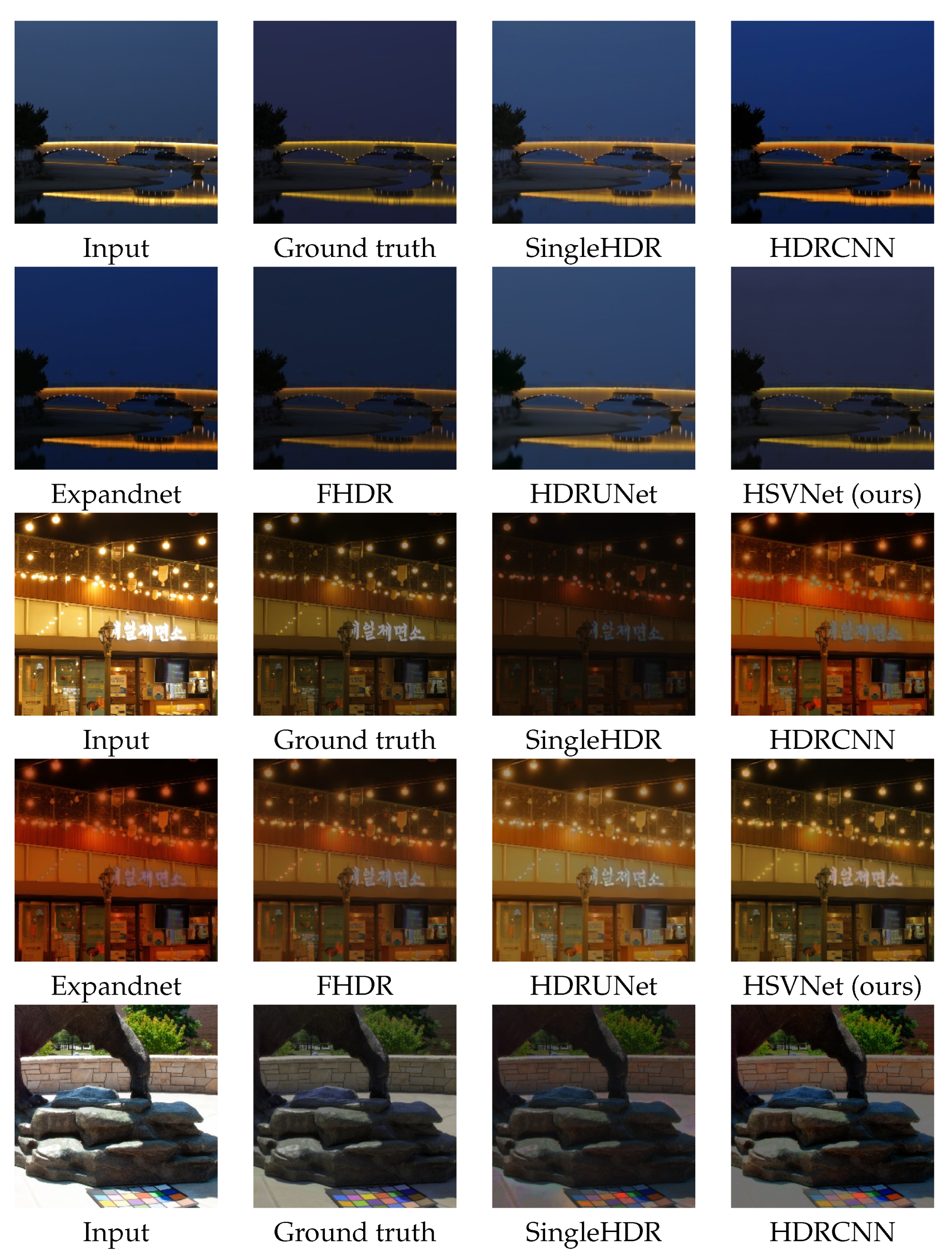
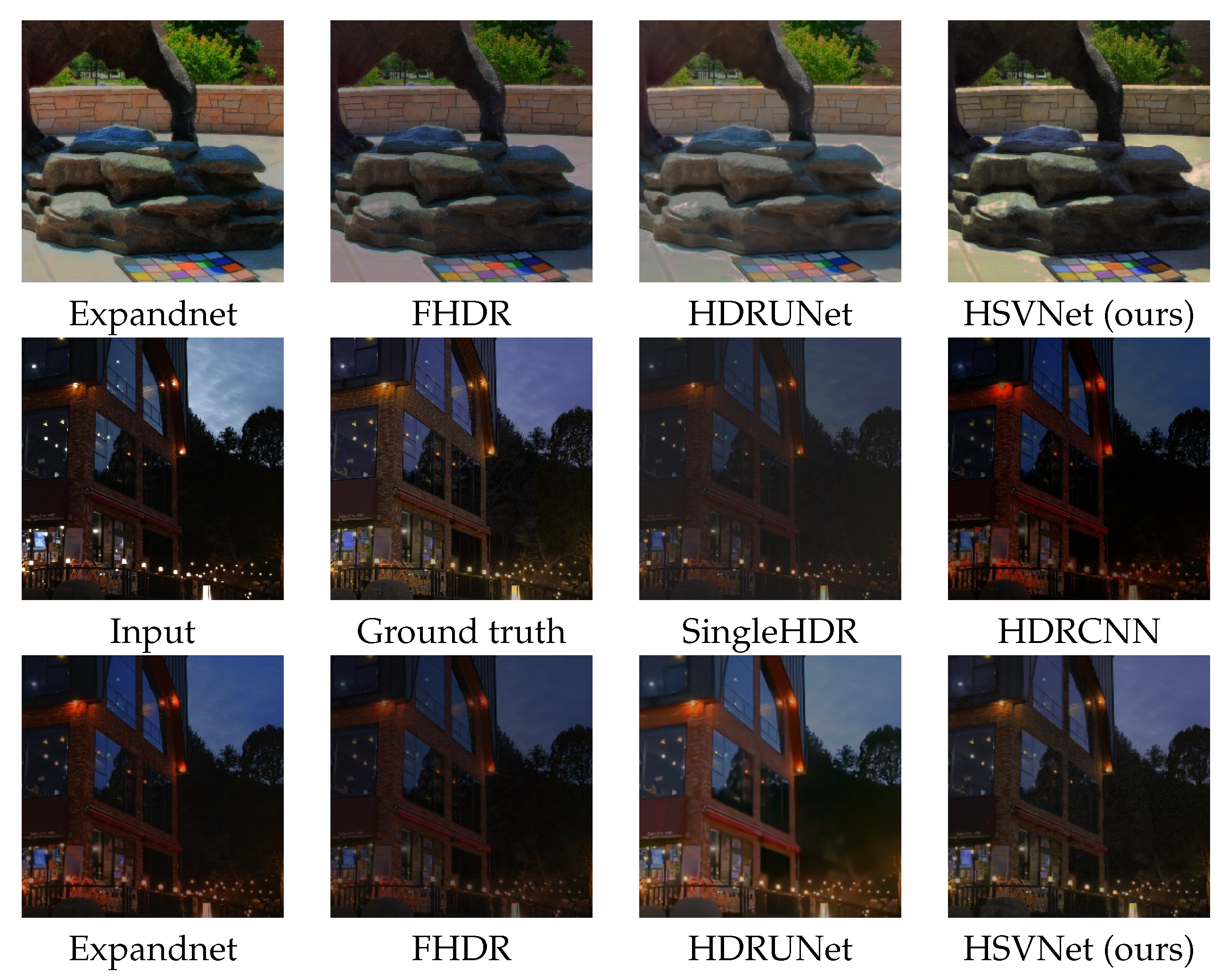
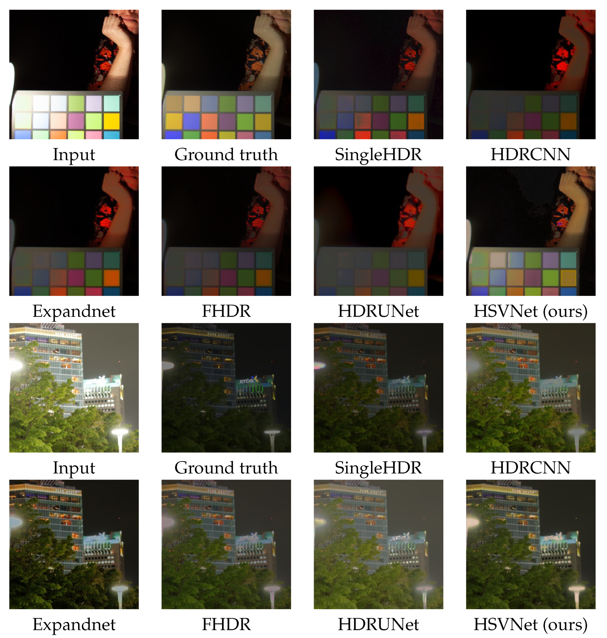
Figure 12 shows the visual comparison of result images between our method, HSVNet, and others. In most cases, HSVNet produces satisfying results which are closest to ground truth images than others. Missing details in both undersaturated and oversaturated areas, as well as the rest areas of input LDR images, are fairly well reconstructed by HSVNet. Especially in the color checkerboard in the fifth and the sixth row, most of colors are restored well even though the checkerboard in the input LDR image is partially undersaturated due to shadows or oversaturated due to sunlight. In addition to the hue of the checker board, saturation and brightness are well recovered by our method.
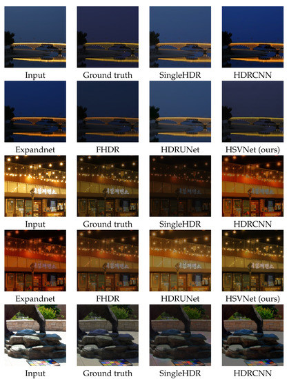

Figure 12.
The result images generated by our method HSVNet and existing methods. The first and the second images are LDR input and the corresponding ground truth HDR images. The next images are the result images from existing methods, SingleHDR, HDRCNN, Expandnet, FHDR, and HDRUNet, respectively. The last image is our HSVNet result image.
Our approach has some limitations, as well. Our method might fail to infer missing detailed information, especially when the majority of the input image is oversaturated. When the input is extremely overexposured (see the first and second row of Figure 13), missing details in input LDR images are not reconstructed well with our method as with all other methods. However, our HSVNet predicts brightness and saturation better than other methods even in extremely oversaturated regions. Additionally, as the input image of the third and the fourth row in Figure 13 is largely overexposed, there is a huge gap between the result images and the ground truth image. There is also a limitation on the resolution of images. Our model is developed not for high resolution, but for relatively low resolution ( pixels). The performance might be debased when the size of the input image is large.

Figure 13.
The result images in which our method did not successfully infer missing details.
7. Conclusions
It is challenging to reconstruct an HDR image from a single random exposure LDR image. To solve this problem, we propose an end-to-end model, HSVNet, which is a U-net-based network. The main difference from previous HDR reconstruction models is using HSV information of images to allow the network to learn the relationships between saturated regions and colors. We develop a customized loss function that is suitable for HSV color space based on characteristics of Hue space to produce satisfying optimal results for human eyes. By applying masks created from S and V information, we restrain the impact of H on saturated regions. The performance quality is proven through comparisons to other existing inverse tone mapping models after experiments.
Author Contributions
Conceptualization, M.J.L., C.-h.R. and C.H.L.; methodology, M.J.L. and C.-h.R.; software, M.J.L.; validation, M.J.L., C.-h.R. and C.H.L.; formal analysis, M.J.L.; investigation, M.J.L.; resources, M.J.L.; writing—original draft preparation, M.J.L.; writing—review and editing, C.H.L.; visualization, M.J.L.; project administration, C.H.L. All authors have read and agreed to the published version of the manuscript.
Funding
This research was partially funded by the National Research Foundation of Korea (NRF) funded by the Ministry of Education grant number NRF-2013R1A1A2060582.
Institutional Review Board Statement
Not applicable.
Informed Consent Statement
Not applicable.
Data Availability Statement
Not applicable.
Conflicts of Interest
The authors declare no conflict of interest.
References
- Yan, Q.; Zhang, L.; Liu, Y.; Zhu, Y.; Sun, J.; Shi, Q.; Zhang, Y. Deep HDR Imaging via A Non-Local Network. IEEE Trans. Image Process. 2020, 29, 4308–4322. [Google Scholar] [CrossRef] [PubMed]
- Jang, H.; Bang, K.; Jang, J.; Hwang, D. Dynamic Range Expansion Using Cumulative Histogram Learning for High Dynamic Range Image Generation. IEEE Access 2020, 8, 38554–38567. [Google Scholar] [CrossRef]
- Banterle, F.; Ledda, P.; Debattista, K.; Chalmers, A. Inverse tone mapping. In Proceedings of the 4th International Conference on Computer Graphics and Interactive Techniques in Australasia and South East Asia, Kuala Lumpur, Malaysia, 29 November–2 December 2006; pp. 349–356. [Google Scholar]
- Rempel, A.G.; Trentacoste, M.; Seetzen, H.; Young, H.D.; Heidrich, W.; Whitehead, L.; Ward, G. Ldr2Hdr: On-the-fly reverse tone mapping of legacy video and photographs. ACM Trans. Graph. 2007, 26, 39-es. [Google Scholar] [CrossRef]
- Kovaleski, R.P.; Oliveira, M.M. High-quality reverse tone mapping for a wide range of exposures. In Proceedings of the 27th SIBGRAPI Conference on Graphics, Patterns and Images, Rio de Janeiro, Brazil, 27–30 August 2014; pp. 49–56. [Google Scholar]
- Wang, L.; Wei, L.-Y.; Zhou, K.; Guo, B.; Shum, H.-Y. High Dynamic Range Image Hallucination. In Proceedings of the Eurographics Symposium on Rendering Techniques, Grenoble, France, 25–27 June 2007; pp. 321–326. [Google Scholar]
- Chen, X.; Liu, Y.; Zhang, Z.; Qiao, Y.; Dong, C. HDRUnet: Single image HDR reconstruction with denoising and dequantization. In Proceedings of the IEEE/CVF Conference on Computer Vision and Pattern Recognition, Nashville, TN, USA, 20–25 June 2021; pp. 354–363. [Google Scholar]
- Eilertsen, G.; Kronander, J.; Denes, G.; Mantiuk, R.K.; Unger, J. HDR image reconstruction from a single exposure using deep CNNs. ACM Trans. Graph. 2017, 36, 1–15. [Google Scholar] [CrossRef]
- Marnerides, D.; Bashford-Rogers, T.; Hatchett, J.; Debattista, K. Expandnet: A deep convolutional neural network for high dynamic range expansion from low dynamic range content. Comput. Graph. Forum 2018, 37, 37–49. [Google Scholar] [CrossRef] [Green Version]
- Liu, Y.-L.; Lai, W.-S.; Chen, Y.-S.; Kao, Y.-L.; Yang, M.-H.; Chuang, Y.-Y.; Huang, J.-B. Single-image HDR reconstruction by learning to reverse the camera pipeline. In Proceedings of the IEEE/CVF Conference on Computer Vision and Pattern Recognition, Seattle, WA, USA, 14–19 June 2020; pp. 1651–1660. [Google Scholar]
- Niu, Y.; Wu, J.; Liu, W.; Guo, W.; Lau, R.W. HDR-GAN: HDR image reconstruction from multi-exposed LDR images with large motions. IEEE Trans. Image Process. 2021, 30, 3885–3896. [Google Scholar] [CrossRef] [PubMed]
- Ye, N.; Huo, Y.; Liu, S.; Li, H. Single exposure high dynamic range image reconstruction based on deep dual-branch network. IEEE Access 2021, 9, 9610–9624. [Google Scholar] [CrossRef]
- Wang, H.; Zhang, T.; Lu, G. Unsupervised HDR Image Reconstruction Based on Over/Under-Exposed LDR Image Pair. In Proceedings of the IEEE International Conference on Multimedia and Expo (ICME), Shenzhen, China, 5–9 July 2021; pp. 1–6. [Google Scholar]
- Fairchild, M.D. The HDR photographic survey. In Proceedings of the Color and Imaging Conference, Albuquerque, NM, USA, 5–9 November 2007; pp. 233–238. [Google Scholar]
- Kim, J.H.; Lee, S.; Jo, S.; Kang, S.-J. End-to-end differentiable learning to HDR image synthesis for multi-exposure images. arXiv 2020, arXiv:2006.15833. [Google Scholar]
- Moriwaki, K.; Yoshihashi, R.; Kawakami, R.; You, S.; Naemura, T. Hybrid loss for learning Single-Image-based HDR reconstruction. arXiv 2018, arXiv:1812.07134. [Google Scholar]
- Debevec, P. A median cut algorithm for light probe sampling. ACM SIGGRAPH Posters 2005, 66, 1–3. [Google Scholar]
- Meylan, L.; Daly, S.; Süsstrunk, S. The reproduction of specular highlights on high dynamic range displays. In Proceedings of the Color and Imaging Conference, Scottsdale, AZ, USA, 6–10 November 2006; Society for Imaging Science and Technology: Springfield, VA, USA, 2006; pp. 333–338. [Google Scholar]
- Masia, B.; Agustin, S.; Fleming, R.W.; Sorkine, O.; Gutierrez, D. Evaluation of Reverse Tone Mapping Through Varying Exposure Conditions. ACM Trans. Graph. 2009, 28, 1–8. [Google Scholar] [CrossRef]
- Masia, B.; Serrano, A.; Gutierrez, D. Dynamic range expansion based on image statistics. Multimed. Tools Appl. 2017, 76, 631–648. [Google Scholar] [CrossRef]
- Huo, Y.; Yang, F.; Dong, L.; Brost, V. Physiological inverse tone mapping based on retina response. Vis. Comput. 2014, 30, 507–517. [Google Scholar] [CrossRef]
- Sen, P.; Kalantari, N.K.; Yaesoubi, M.; Darabi, S.; Goldman, D.B.; Shechtman, E. Robust patch-based HDR reconstruction of dynamic scenes. ACM Trans. Graph. 2012, 31, 1–11. [Google Scholar] [CrossRef]
- Yang, X.; Xu, K.; Song, Y.; Zhang, Q.; Wei, X.; Lau, R.W. Image correction via deep reciprocating HDR transformation. In Proceedings of the IEEE Conference on Computer Vision and Pattern Recognition, Salt Lake City, UT, USA, 18–23 June 2018; pp. 1798–1807. [Google Scholar]
- Khan, Z.; Khanna, M.; Raman, S. FHDR: HDR image reconstruction from a single LDR image using feedback network. In Proceedings of the IEEE Global Conference on Signal and Information Processing (GlobalSIP), Ottawa, ON, Canada, 11 November 2019; pp. 1–5. [Google Scholar]
- Simonyan, K.; Zisserman, A. Very Deep Convolutional Networks for Large-Scale Image Recognition. In Proceedings of the International Conference on Learning Representations (ICLR), San Diego, CA, USA, 7–9 May 2015. [Google Scholar]
- Santos, M.S.; Tsang, I.; Kalantari, N.K. Single image HDR reconstruction using a CNN with masked features and perceptual loss. ACM Trans. Graph. (TOG) 2020, 39, 1–10. [Google Scholar] [CrossRef]
- Li, J.; Fang, P. HDRNET: Single-image-based HDR reconstruction using channel attention CNN. In Proceedings of the 2019 4th International Conference on Multimedia Systems and Signal Processing, Guangzhou, China, 10–12 May 2019; pp. 119–124. [Google Scholar]
- Goodfellow, I.; Pouget-Abadie, J.; Mirza, M.; Xu, B.; Warde-Farley, D.; Ozair, S.; Courville, A.; Bengio, Y. Generative adversarial nets. In Proceedings of the Advances in Neural Information Processing Systems, Montreal, QC, Canada, 8–13 December 2014; pp. 2672–2680. [Google Scholar]
- Kim, S.Y.; Oh, J.; Kim, M. JSI-GAN: GAN-based joint super-resolution and inverse tone-mapping with pixel-wise task-specific filters for UHD HDR video. In Proceedings of the AAAI Conference on Artificial Intelligence, New York, NY, USA, 7–12 February 2020; Volume 34, pp. 11287–11295. [Google Scholar]
- Marnerides, D.; Bashford-Rogers, T.; Debattista, K. Deep HDR Hallucination for Inverse Tone Mapping. Sensors 2021, 12, 4032. [Google Scholar] [CrossRef]
- Goodfellow, I.; Bengio, Y.; Courville, A. Deep Learning; MIT Press: Cambridge, MA, USA, 2020. [Google Scholar]
- Vincent, P.; Larochelle, H.; Bengio, Y.; Manzagol, P.A. Extracting and composing robust features with denoising autoencoders. In Proceedings of the 25th International Conference on Machine Learning, Helsinki, Finland, 5–9 July 2008; pp. 1096–1103. [Google Scholar]
- Ronneberger, O.; Fischer, P.; Brox, T. U-net: Convolutional networks for biomedical image segmentation. In Proceedings of the International Conference on Medical Image Computing and Computer-Assisted Intervention, Munich, Germany, 5–9 October 2015; pp. 234–241. [Google Scholar]
- Dong, L.F.; Gan, Y.Z.; Mao, X.L.; Yang, Y.B.; Shen, C. Learning deep representations using convolutional auto-encoders with symmetric skip connections. In Proceedings of the IEEE International Conference on Acoustics, Speech and Signal Processing (ICASSP), Calgary, AB, Canada, 15–20 April 2018; pp. 3006–3010. [Google Scholar]
- Gonzalez, R.C.; Woods, R.E. Color Image Processing. In Digital Image Processing, 2nd ed.; Prentice Hall: Hoboken, NJ, USA, 2002; pp. 295–297. [Google Scholar]
- Willmott, C.J.; Matsuura, K. Advantages of the mean absolute error (MAE) over the root mean square error (RMSE) in assessing average model performance. Clim. Res. 2005, 30, 79–82. [Google Scholar] [CrossRef]
- Narwaria, M.; Mantiuk, R.; Da Silva, M.P.; Callet, P.L. HDR-VDP-2.2: A calibrated method for objective quality prediction of high-dynamic range and standard images. J. Electron. Imaging 2015, 24, 010501. [Google Scholar] [CrossRef] [Green Version]
- Mantiuk, R.; Azimi, M. PU21: A novel perceptually uniform encoding for adapting existing quality metrics for HDR. In Proceedings of the 2021 Picture Coding Symposium (PCS), Bristol, UK, 29 June–2 July 2021; pp. 1–5. [Google Scholar]
- Hammersley, J. Monte Carlo Methods; Springer Science and Business Media: Berlin/Heidelberg, Germany, 2013. [Google Scholar]


Publisher’s Note: MDPI stays neutral with regard to jurisdictional claims in published maps and institutional affiliations. |
© 2022 by the authors. Licensee MDPI, Basel, Switzerland. This article is an open access article distributed under the terms and conditions of the Creative Commons Attribution (CC BY) license (https://creativecommons.org/licenses/by/4.0/).