Multi-Directional Shape Change Analysis of Biotensegrity Model Mimicking Human Spine Curvature

Featured Application

The advantageous characteristics of the flexibility and versatility of the movement of spine biotensegrity models can be further studied for potential application in the shape change control of deployable structures and flexible arms in the robotic industry.

Abstract

This paper presents a numerical strategy for the shape change analysis of spine biotensegrity models in multi-directional modes. The formulation of incremental equilibrium equations and optimization problem for shape change analysis via the forced elongation of cables to achieve the target coordinates of the monitored nodes of spine biotensegrity models are presented. The distance between the monitored nodes and the target coordinates is chosen as the objective function which is minimized subject to inequality constraints on member axial forces and cable forced elongation. Three spine biotensegrity models were analyzed to validate the effectiveness of the proposed method. The deformation characteristics of the Class-1 four-stage biotensegrity models mimicking the natural curvature of the human spine were investigated. A highly successful rate in achieving the target coordinates was observed in a total of 258 analysis cases, with percentages of 99.9%, 99.9% and 98.9% for shape change analysis involving uni-, bi- and tri-directional modes, respectively. The results show that the spine biotensegrity models have more flexibility in undergoing bending in comparison with axial deformation. With the established shape change strategy, the flexibility and versatility of the movement of spine biotensegrity models can be further studied for potential application in the shape change control of deployable structures together with the use of IoT.

1. Introduction

The principle of biotensegrity is an application of the concept of tensegrity in explaining the anatomy and physiology of biological systems which has been studied since 1980s. Biotensegrity consisting of compressive (i.e., vertebrae) and tensional (i.e., fascial, muscle, tendon) components exhibits stable form, prestressed condition at rest and effective transmission of forces within the system. Extensive research investigations on biotensegrity based biomechanical models, particularly cellular, molecular, organ and tissue, organisms and fascial biotensegrity, as well as the principle of biotensegrity in cellular mechanical signal transduction (mechanotransduction), were reported [1,2]. To date, biotensegrity as a model emulated from the forms and functions of complex biological systems has been suggested for several potential applications such as in medical technology [3], health care practices [4] and engineering applications [5].

Characteristics, such as the ability to self-assemble and perform global deformations upon loadings while at the same time maintaining their stability, have been attracting increasing interest on the shape change of tensegrity. The deformation of tensegrities to achieve shape change is basically generated based on the member length actuation, change in prestress and alteration of the structural stiffness of tensegrities. Most of the previous studies implemented static or quasi-static deployment analysis owing to the complicated mechanical properties of the tensegrities [6]. The shape change of tensegrity was solved as a quasi-static problem during the sufficiently slow deployment process [7,8,9]. The solutions to the quasi-static problems of tensegrities are commonly proposed by employing numerical, analytical and optimization algorithms. Zhang, et al. [10] derived a non-linear finite element formulation for the quasi-static deployment of clustered tensegrities based on a co-rotational approach. Veuve, et al. [11] investigated a control methodology to connect two half bridges through the changes of cable length employing a combination of stochastic search and quasi-static analyses. The deployment of the footbridges was solved based on the distance between a pair of nodal coordinates of two mid-span connectors. Kan et al. [7] carried out both quasi-static and dynamic analyses for a clustered tensegrity beam and a four-stage tensegrity tower incorporating sliding cable elements. Using an energy-based approach for system equilibriums and a nonlinear finite element model, the trajectory and stress distribution of two foldable tensegrity-membrane systems during deployment was investigated [12]. Zhu and Deng [8] applied quasi-static assumptions for determining the member length actuation of a cantilever tensegrity based on the variation in the structural load-carrying stiffness. Yıldız and Lesieutre [13] developed general analysis methods for n-strut cylindrical Class-1 and Class-2 deployable tensegrity booms, with the assumption of quasi-static motion. A shape control method employing a dynamic relaxation-based motion tracking algorithm suitable for both quasi-static and dynamic process was proposed in [9]. Nonetheless, a study on shape change analysis of biotensegrity, especially for deployable structures, has not been found.

Instead, many have studied the shape change of biotensegrity for robotic and automation applications. A class 2 biotensegrity underwater robot was designed and fabricated with stiffness approximating that of the real fish [14]. The flipping of the fish tail was performed by tuning the bending stiffness of the robot body, which was formulated based on the virtual work method. Using the force density method to solve the inverse kinematics, a modular tensegrity robot inspired by the vertebrae morphologies to grasp objects was developed [15]. An investigation on the motion patterns of a flexible biotensegrity manipulator mimicking the shrinking behavior of octopus tentacles was also conducted [16]. Although many studies of biotensegrity robots have been conducted through numerical and experimental works, the static and kinematic problems are hardly solved due to highly constrained coupling systems, particularly when subjected to an external load [17].

Inspired by the flexible and versatile multi-directional movement ability of the human spine, the shape change process of three Class-1 spine biotensegrity models is the focus of this study. The proposed models preserve the slenderness and natural curvature of the human spine in the geometry, particularly emphasizing the stabilizing network of the spinal column and muscle through the biotensegrity principle. The aims of the study are two-fold: (i) evaluation of the effectiveness of the shape change control strategy proposed by the authors [18] when applied on the spine biotensegrity models, and (ii) investigation of the potential deformation characteristics of the spine biotensegrity models in uni-, bi- and tri-directional modes. The outcome of this study can be possibly extended to the shape change control of bio-tensegrity models where sensors and Internet of Things (IoT) technology are made use of to perform automated tasks.

This paper is structured as follows: Section 2 explains the anatomical parameters and topologies of the spine biotensegrity models. Section 3 presents the shape change strategies—particularly the formulation of the incremental equilibrium equation, the optimization method via sequential quadratic programming and the shape change analysis algorithm. Section 4 discusses the effectiveness of the proposed shape change method through numerical examples of spine biotensegrity models. Lastly, conclusions are presented in Section 5.

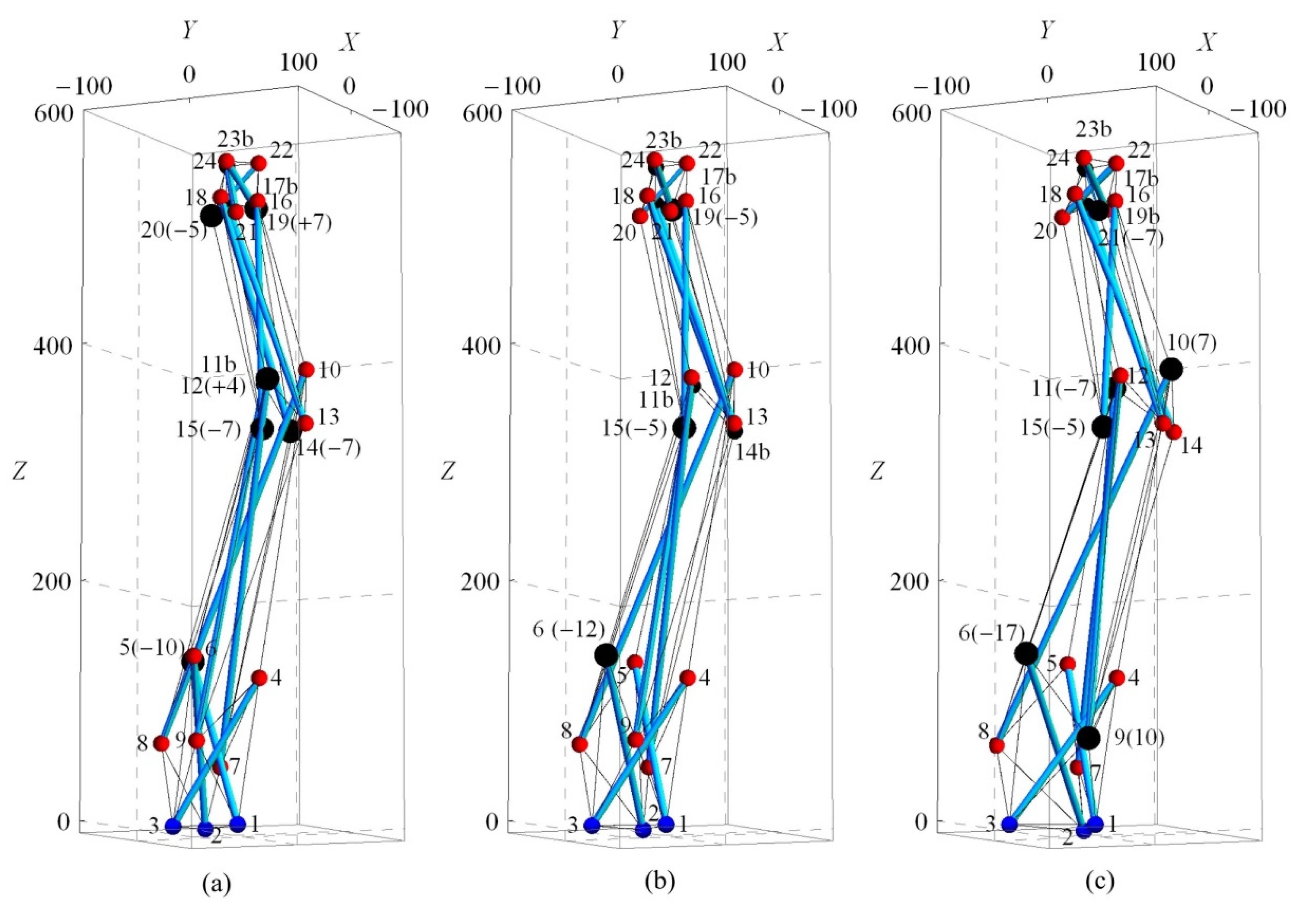
2. Spine Biotensegrity Models

Four-stage spine biotensegrity models, SB1, SB2, and SB3 proposed by Oh, Choong, Nishimura and Kim [5], were used in this study. This section briefly explains the anatomical parameters and topologies of the spine biotensegrity models. In this study, the biotensegrity model was modelled by mimicking the topology of the human spine where the width, height and the natural curvature of actual human spine vertebrae anatomical parameters are taken into consideration. The exact location of the muscles, fascial and ligaments as well as other parts of the body connected to the spine are not considered in the modelling. The Class-1 tensegrity mast is adopted to mimic the human spine represented by vertebrae (i.e., struts) which are gapped and cushioned by intervertebral discs and well surrounded by muscles (i.e., cables). Real human spine anatomical parameters studied by Busscher, et al. [19] were adopted for the geometrical input data of spine biotensegrity models. These anatomical parameters are the vertebral end-plate width, vertebral central body height and intervertebral disc height (see Figure 1). The aggregation of both vertebral central body height and intervertebral disc height characterizes the height of the spine biotensegrity model, whereas the accumulation of intervertebral disc height is modelled using the saddle height which corresponds to the vertical distance between the upper triangular surface of the lower cell and the lower triangular surface of the upper cell in the biotensegrity model. The tapered section properties of a human spine are incorporated into the spine biotensegrity models. A total of twenty-two vertebrae, particularly vertebrae C3–C7, T1–T12 and L1–L5 within the cervical, thoracic and lumbar regions, respectively, were considered in the spine biotensegrity models. The spine biotensegrity models also incorporated the natural curvature of the human spine with cervical lordosis at an apice AP1 of 20.1°, thoracic kyphosis at an apice AP2 of 34.5° and lumbar lordosis at an apice AP3 of 29.2°.

The SB1, SB2 and SB3 models were differentiated in terms of the different sizes of triangular cells, represented by half of their triangular vertex angles (θ) with values of 20°, 30° and 40°, respectively (Figure 2). The triangular cell was chosen for the spine biotensegrity models due to its simple geometry. All of the SB models have the same magnitude of triangle altitude, d, which was characterized by the vertebral end-plate width of the vertebrae. The spine biotensegrity model is made up of four triangular cells which are stacked on each other. Each triangular cell is bounded by triangular surfaces at the lower and upper end, respectively (Figure 2). In total, there are eight triangular surfaces in the spine tensegrity model: one at the base, two at each of the three apices and one at the top. Figure 2 shows the geometry of a triangular cell in the global Cartesian coordinate system O_o-X_oY_oZ_o. The position vector of nodal coordinates is denoted as X. The origins of the local Cartesian system O_i−1-X_i−1Y_i−1Z_i−1 and O_i-X_iY_iZ_i are positioned at the centroid of the lower (X_6i-5 X_6i-4 X_6i-3) and upper triangular surfaces (X_6i−2 X_6i−1 X_6i) of ith (i = 1, 2, …, 4) triangular cell, respectively. Each spine biotensegrity model consists of sixty-nine elements (i.e., twelve struts and fifty-seven cables). Details and the form-finding strategy of the self-equilibrated human spine biotensegrity models can be found in Oh, Choong, Nishimura and Kim [5]. Figure 3 shows the model of spine biotensegrity used for shape change analysis in this study. The topologies, material properties and configurations of these models are shown in

Table A1. Nodal coordinates of SB1, SB2 and SB3 [5].

Nodes	SB1			SB2			SB3
	x	y	z	x	y	z	x	y	z
1	9.33	−1.23	0	9.33	-1.23	0	9.33	−1.23	0
2	−24.01	−48.3	0	−35.34	−45.27	0	−49.24	-41.54	0
3	14.67	−58.67	0	26	−61.7	0	39.91	−65.43	0
4	−8.9	9.49	123.78	−8.9	9.49	123.78	−8.9	9.49	123.78
5	−14.71	−55.48	141.36	−25.95	−48.49	141.36	−39.72	−52.18	141.36
6	23.61	−35.21	141.36	34.85	−44.2	141.36	48.62	−45.51	141.36
7	−33.22	-39	52.83	−33.22	−39	52.83	−33.22	−39	52.83
8	11.48	−71.52	70.41	8.47	−82.75	70.41	4.77	−96.53	70.41
9	21.75	−33.19	70.41	24.76	−21.96	70.41	28.45	1.82	70.41
10	−10.04	52.87	382.82	−10.04	52.87	382.82	−10.04	59.87	382.82
11	−7.19	14.89	372.81	−14.34	11.56	372.81	−23.12	0.46	372.81
12	17.23	30.28	372.81	24.38	29.61	372.81	33.16	33.7	372.81
13	14.15	63.71	332.85	14.15	63.71	332.85	14.15	63.71	332.85
14	−18.11	34.13	332.85	−24.57	45.65	332.85	−32.51	51.21	332.85
15	3.96	18.67	332.85	10.42	16.15	332.85	18.36	10.49	332.85
16	−5.08	10.05	531.04	−5.08	10.05	531.04	−5.08	10.05	531.04
17	−7.84	−21.15	533.31	−13.91	−22.77	533.31	−21.37	−24.77	533.31
18	12.91	−15.59	533.31	18.99	−13.96	533.31	26.44	−11.96	533.31
19	−18.29	2.21	527.57	−18.29	−9.79	527.57	−18.29	−4.79	527.57
20	6.37	−27.52	519.59	4.74	−28.59	519.59	2.74	−36.05	519.59
21	11.93	−1.77	519.59	13.56	4.31	519.59	15.55	4.77	519.59
22	−7.58	9.77	564.29	−7.58	9.77	564.29	−7.58	9.77	564.29
23	−5.12	−18.78	564.29	−10.33	−21.21	564.29	−16.74	−24.21	564.29
24	12.7	−10.47	564.29	17.91	−8.04	564.29	24.33	−5.05	564.29

Note: Unit in mm.

and

Table A2. Material properties.

Elastic Modulus, E (MPa)	Strut and Cable Yield Stress, σs, σc (MPa)	Density, γ (kg/mm3)	Strut Cross Sectional Area, As (mm2)	Cable Cross Sectional Area, Ac (mm2)
20,000	250	7.7 × 10-6	50.30	3.14

.

3. Shape Change Strategies for Spine Biotensegrity Models

The analysis strategy used in the numerical simulation of the shape change of bio-tensegrity is briefly summarized in this section. In order to solve the convex problem, constraints on member axial forces are imposed so that buckling does not occur. Moreover, strictly minimizing the shape control path is not considered in this study. Therefore, we adopted the numerical strategy of the sequential quadratic programming method in which the objective function described in Reference 18 is the distance from the target position. A detailed description of the shape change analysis strategy can be found in the author’s previous work [18].

In the numerical simulation of shape change, the following states are involved: initial state, deformed state, shape change state and target state. The initial state corresponds to the state obtained from the form-finding analysis without any constraints and external forces. At the deformed state, the model undergoes linear elastic deformation with the imposition of constraints and self-weight on the initial state. At the shape change state, the model undergoes shape change by means of forced elongation in cables. The target state corresponds to the state to be achieved where coordinates of a set of nodes are prescribed. The shape change process of the spine biotensegrity model starts from the deformed state and ends when the target state is achieved.

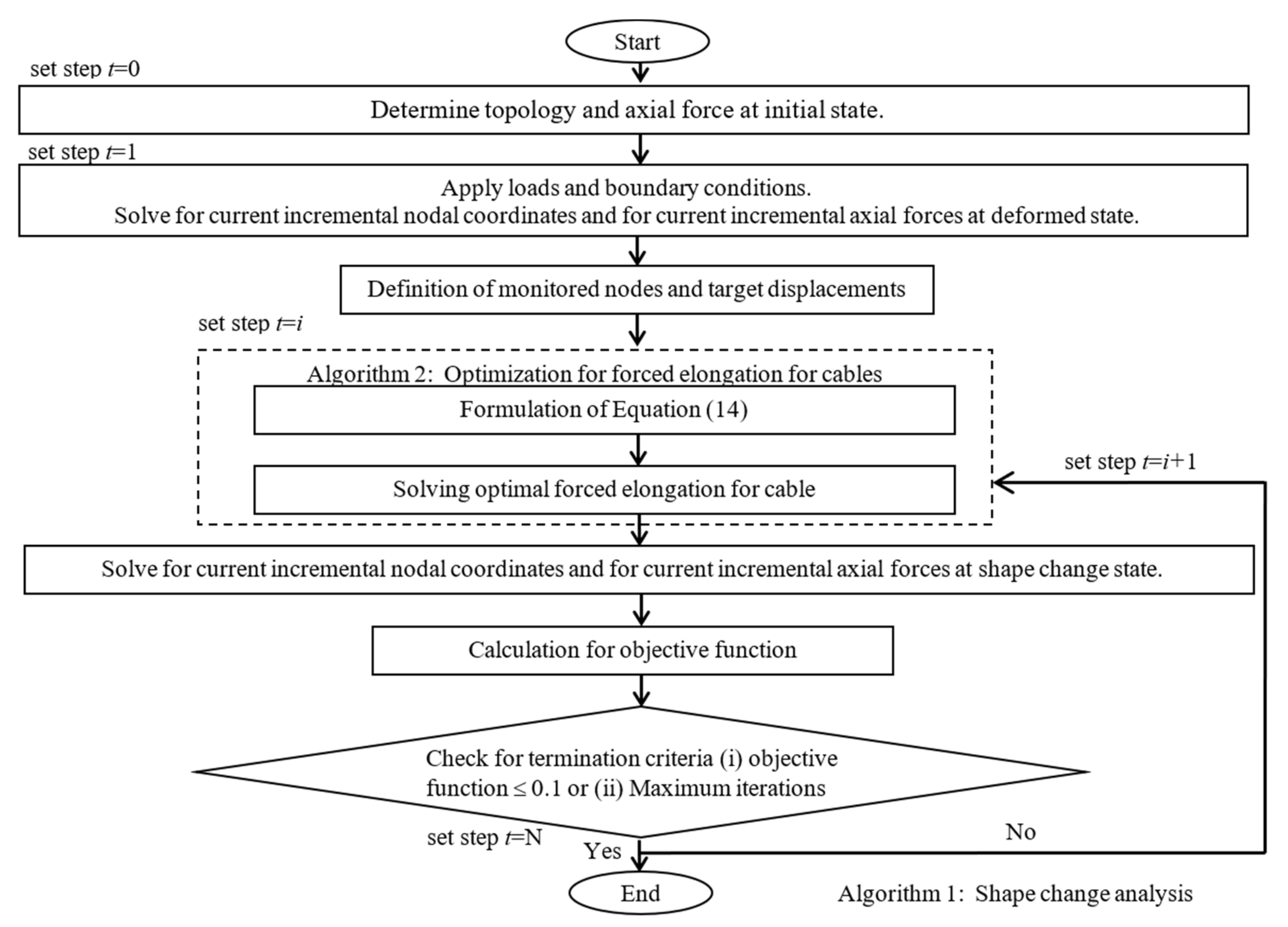
3.1. Formulation of Incremental Equilibrium Equations

This section shows the formulation of incremental equilibrium equations for spine biotensegrity models with m elements, n nodes, n_c constraints and n_u (3n−n_c) unconstrained degree of freedoms. The formulation is generally based on the static equilibrium equation, which could be expressed as follows:

$$\mathbf{F}=\mathbf{B}\mathbf{n}$$

(1)

where B is a n_u × m matrix of directional cosines, F is a vector of nodal forces with size n_u and n is a vector of axial forces with size m. The vector of directional cosine λ for a member of a biotensegrity model at incremental step t could be written as follows:

$${}_{}{}^t\mathit{\lambda }=\frac{\left({}_{}{}^{t-1}\mathit{x}{}_j-{}_{}{}^{t-1}\mathit{x}{}_i\right)}{{}_{}{}^{t-1}l+{}_{}{}^{t-1}u}$$

(2)

where l, u, x_i and x_j are the initial geometrical inputs, particularly the length after forced elongation, elastic elongation, nodal coordinate at nodes i and j, obtained from the previous step t − 1.

The incremental equilibrium equation for the entire structure could be obtained by the differentiation of Equation (1) as follows:

$${}_{}{}^t\dot{\mathbf{F}}={}^t\dot{\mathbf{B}} {}^t\mathbf{n}+{}^t\mathbf{B} {}^t\dot{\mathbf{n}}$$

(3)

Contents of equilibrium equations at the member level which are used in the summation process to obtain Equation (3) are shown as follows:

$$\left\{\begin{array}{c}{{}^t\dot{\mathbf{f}}}_i\\ {{}^t\dot{\mathbf{f}}}_j\end{array}\right\}=\left[\begin{array}{c}{-}^t\dot{\lambda }\\ {}^t\dot{\lambda }\end{array}\right]{}_{}{}^t\mathbf{n}+\left[\begin{array}{c}-{}_{}{}^t\lambda \\ {}_{}{}^t\lambda \end{array}\right]{}^t\dot{\mathbf{n}}$$

(4)

where the f_i, f_j are vectors of nodal force at end i and j of the member.

The first term on the right-hand side of Equation (4) could be expressed as follows:

$$[\begin{array}{c}-{}_{}{}^t\dot{\lambda }\\ {}_{}{}^t\dot{\lambda }\end{array}]{}^t\mathbf{n}={}^t\mathbf{k}{}_g\left\{\begin{array}{c}{}_{}{}^{t}x{}_i\\ {}_{}{}^{t}x{}_j\end{array}\right\}$$

(5)

where ^tk_g is the 6 × 6 geometrical stiffness matrix of which the contents are given as follows:

$${}_{}{}^t\mathbf{k}{}_g=\frac{{}_{}{}^{t-1}n}{{}_{}{}^{t-1}l+{}_{}{}^{t-1}u}\left[\begin{array}{cc}\left[{\mathbf{I}}_3-{}_{}{}^t\mathbf{\lambda }{}_{}{}^t\mathbf{\lambda }{}^{\mathrm{T}}\right]& -\left[{\mathbf{I}}_3-{}_{}{}^t\mathbf{\lambda }{}_{}{}^t\mathbf{\lambda }{}^{\mathrm{T}}\right]\\ -\left[{\mathbf{I}}_3-{}_{}{}^t\mathbf{\lambda }{}_{}{}^t\mathbf{\lambda }{}^{\mathrm{T}}\right]& \left[{\mathbf{I}}_3-{}_{}{}^t\mathbf{\lambda }{}_{}{}^t\mathbf{\lambda }{}^{\mathrm{T}}\right]\end{array}\right]$$

(6)

where I₃ is a 3 × 3 identity matrix.

The second term on the right-hand side of Equation (4) could be expressed as

$$\left\{\begin{array}{c}-{}_{}{}^t\lambda \\ {}_{}{}^t\lambda \end{array}\right\}{}^t\dot{\mathbf{n}}={}_{}{}^t\mathbf{k}{}_e\left\{\begin{array}{c}{}_{}{}^{t}x{}_i\\ {}_{}{}^{t}x{}_j\end{array}\right\}-\left\{\begin{array}{c}-{}_{}{}^t\lambda \\ {}_{}{}^t\lambda \end{array}\right\}\frac{EA}{{}_{}{}^{t-1}l}\left(1+\frac{{}_{}{}^{t-1}u}{{}_{}{}^{t-1}l}\right){}_{}{}^t\dot{l}$$

(7)

where ^tk_e is the 6 × 6 linear stiffness matrix which is given by the following expression:

$${}_{}{}^t\mathbf{k}{}_e=\frac{EA}{{}_{}{}^{t-1}l{}^{}}\left[\begin{array}{cc}{}_{}{}^t\mathbf{\lambda }{}_{}{}^t\mathbf{\lambda }{}^{\mathrm{T}}& -{}_{}{}^t\mathbf{\lambda }{}_{}{}^t\mathbf{\lambda }{}^{\mathrm{T}}\\ -{}_{}{}^t\mathbf{\lambda }{}_{}{}^t\mathbf{\lambda }{}^{\mathrm{T}}& {}_{}{}^t\mathbf{\lambda }{}_{}{}^t\mathbf{\lambda }{}^{\mathrm{T}}\end{array}\right]$$

(8)

Superimposing Equation (4), rewritten Equation (3) gives the incremental equation for the entire structure as follows:

$$\begin{array}{c}{}_{}{}^t\dot{\mathbf{F}}={}_{}{}^t\mathbf{K}{}_{}{}^t\dot{\mathit{x}}-{}_{}{}^t\mathbf{B}{}_{}{}^t\mathbf{C}{}_L{}_{}{}^t\dot{\mathbf{l}}\\ {}_{}{}^t\mathbf{K}={\displaystyle {\displaystyle \sum }_{\mathrm{member}}}\left({}_{}{}^t\mathbf{k}{}_e+{}_{}{}^t\mathbf{k}{}_g\right)\end{array}$$

(9)

where ${}_{}{}^t\mathbf{K}$ is the structure tangent stiffness matrix and ${}_{}{}^t\dot{\mathbf{l}}$ is the vector of the incremental force elongation of cables. ^tC_L is a m × m matrix which could be further expressed as follows:

$${}_{}{}^t\mathit{C}{}_L=\left[\begin{array}{cccc}\frac{E_1{A}_1}{{}_{}{}^{t-1}{l}_1{}^{}}& & & \\ & \frac{E_1{A}_1}{{}_{}{}^{t-1}{l}_1{}^{}}& & \\ & & \ddots & \\ & & & \frac{E_{\mathrm{m}}{A}_{\mathrm{m}}}{{}_{}{}^{t-1}{l}_{\mathrm{m}}{}^{}}\end{array}\right]+\left[\begin{array}{cccc}\frac{E_1{A}_1}{{}_{}{}^{t-1}{l}_1{}^{}}\left(\frac{{}_{}{}^{t-1}{u}_1}{{}_{}{}^{t-1}{l}_1{}^{}}\right)& & & \\ & \frac{E_2{A}_2}{{}_{}{}^{t-1}{l}_2{}^{}}\left(\frac{{}_{}{}^{t-1}{u}_2}{{}_{}{}^{t-1}{l}_2{}^{}}\right)& & \\ & & \ddots & \\ & & & \frac{E_{\mathrm{m}}{A}_{\mathrm{m}}}{{}_{}{}^{t-1}{l}_{\mathrm{m}}{}^{}}\left(\frac{{}_{}{}^{t-1}{u}_{\mathrm{m}}}{{}_{}{}^{t-1}{l}_{\mathrm{m}}{}^{}}\right)\end{array}\right]$$

(10)

Since a tensegrity under feasible prestress is a stable structure, the inverse of ${}_{}{}^t\mathbf{K}$ exists. The vector of incremental coordinates for the entire structure ${{}_{}{}^t\dot{\mathbf{x}}}_G$ could be obtained by solving Equation (9) with ${}_{}{}^t\dot{\mathbf{F}}=0$:

$${{}_{}{}^t\dot{\mathbf{x}}}_G={}_{}{}^t\mathbf{K}{}^{-1}{}_{}{}^t\mathbf{B}{}_{}{}^t\mathbf{C}{}_L{}_{}{}^t\dot{\mathbf{l}}$$

(11)

The vector of incremental axial force could be expressed as follows:

$$\begin{array}{c}{}_{}{}^t\dot{\mathbf{n}}={}_{}{}^t\mathbf{D}{}_2{}_{}{}^t\dot{\mathbf{l}}\\ {}_{}{}^t\mathbf{D}{}_2=\left({}_{}{}^t\mathbf{C}{}_1{}_{}{}^t\mathbf{B}{}^T{}_{}{}^t\mathbf{K}{}^{-1}{}_{}{}^t\mathbf{B}-{\mathbf{I}}_m\right){}_{}{}^t\mathbf{C}{}_L\end{array}$$

(12)

3.2. Optimization by Sequential Quadratic Programming

The shape change of the spine biotensegrity model is achieved via the changeable length of cables which is enforced in numerical analysis with the forced elongation of cables. The shape change strategy is planned for a set of identified monitored nodes to advance from their initial position to target positions. This advancement to target position represented by a set of prescribed coordinates of the monitored nodes is achieved by minimizing the following objective function:

$$\min f\left(\mathit{x}\right)=|{{}_{}{}^t\mathit{x}}^{\prime }-\overline{\mathit{x}}|$$

(13)

where $\overline{\mathit{x}}$ is the prescribed target coordinates and ${{}^t\mathit{x}}^{\prime }={{}^{t-1}\mathit{x}}^{\prime }+{{}^t\dot{\mathit{x}}}^{\prime }$ is the current coordinates for all of the specified monitored nodes at current step t during the shape change analysis.

The Sequential Quadratic Programming (SQP) method is used to solve the nonlinear optimization problem as shown in Equation (13). The quadratic programming sub-problem can be written as follows:

$$\begin{array}{c}\underset{xϵR^n}{\min }f\left(\mathit{x}\right)={\mathbf{g}}^T{}_{}{}^t\dot{\mathbf{l}}+\frac{1}{2}{}_{}{}^t\dot{\mathbf{l}}{}_{}{}^{\mathrm{T}}\mathbf{H}{}_{}{}^t\dot{\mathbf{l}}\\ \mathrm{subject}\mathrm{to}{\mathbf{A}}_2{}_{}{}^t\dot{\mathbf{l}}\ge {\mathbf{b}}_2\\ \mathrm{where}\\ \mathbf{g}={\mathbf{B}}_2{}^{\mathrm{T}}\left({{}_{}{}^{t-1}\mathit{x}}^{\prime }-\overline{\mathit{x}}\right)\\ \mathbf{H}={\mathbf{B}}_2{}^{\mathbf{T}}{\mathbf{B}}_2\end{array}$$

(14)

${}_{}{}^t\dot{\mathbf{l}}$ is a m_cf × 1 vector of incremental forced elongation which corresponds to the optimization variable, and H is a positive-definite approximation of the Hessian matrix of the Lagrangian function. m_cf is the number of cables excluding the undeformed cables. Matrix A₂ and vector b₂ are the inequality constraints corresponding to the limitation in allowable axial forces and forced elongation, respectively, as follows:

$${\mathbf{A}}_2=\left\{\begin{array}{c}{\mathit{D}}_2\\ \dots \\ -{\mathit{D}}_2\\ \dots \\ {\mathit{I}}_{mcf}\\ \dots \\ -{\mathit{I}}_{mcf}\end{array}\right\};{\mathbf{b}}_2=\left\{\begin{array}{c}{\mathit{n}}_L-{}_{}{}^{t-1}\mathit{n}\\ \dots \\ -\left({\mathit{n}}_U-{}_{}{}^{t-1}\mathit{n}\right)\\ \dots \\ -d_{cl}\\ \dots \\ -d_{cl}\end{array}\right\}$$

(15)

where A₂ is a (2m + 2m_cf) × m_cf matrix and b₂ is a (2m + 2m_cf) × 1 vector. ${\mathit{n}}_L,{}^{t-1}\mathit{n},{\mathit{n}}_U$ are vectors of the lower limit of axial force, axial force at step (t − 1) and upper limit of axial force, respectively. d_cl (with d_cl > 0) is the limit for length imposed on the magnitude of forced elongation ${}_{}{}^t\dot{\mathbf{l}}$.

For elastic material properties, the lower and upper axial force limits for cables and struts are defined as:

$$0\le n_c\le {\mathsf{\sigma }}_c{A}_c$$

(16)

$$\max \left\{-\frac{{\pi }^2{E}_s{I}_s}{l_s{}^2},-{\mathsf{\sigma }}_s{A}_s\right\}\le n_s\le {\mathsf{\sigma }}_s{A}_s$$

(17)

where n_c, σ_c and A_c are axial forces, the yield stress and the cross-sectional area for cable elements, respectively; n_s, E_s, I_s, L_s, σ_s and A_s are axial forces, Young modulus, the moment of inertia, the element current length, the yield stress and the cross sectional area for strut elements, respectively. In this study, all strut elements have a circular cross-section.

The obtained converged ${}_{}{}^t\dot{\mathbf{l}}$ is then used in each incremental step of shape change analysis to determine the updated incremental nodal coordinates in Equation (11) and the incremental axial forces in Equation (12). Figure 4 shows the proposed algorithm for the shape change analysis of tensegrity.

4. Numerical Examples

The proposed algorithm is applied to three spine biotensegrity models (i.e., SB1, SB2 and SB3) with cases of target displacement in uni-, bi- and tri- directional modes. In the uni-directional mode case, a single degree of freedom (x, y or z) of the monitored nodes is prescribed (Figure 5a), with the series denoted as Xn, Xp, Yn, Yp, Zn and Zp. In the bi-directional mode case, both the coordinates of the x and y directions of the monitor nodes are prescribed (Figure 5b), with analysis cases generally represented as XY and specifically denoted as XpYp, XnYp, XnYn and XpYn. For the tri-directional mode case, the shape change analysis cases are denoted as XY, or, specifically, XpYp, XnYp, XnYn and XpYn and then followed by Z, Zn or Zp. In the notation of analysis cases, the capital letters denote the corresponding degree of freedom where the displacement is prescribed (i.e., in x, y and z directions), and the lowercase n and p denote the negative and positive directions of the prescribed displacement, respectively. The number of analysis cases in uni-, bi- and tri- directional modes for SB1, SB2 and SB3 models are 54, 36 and 168 cases, respectively.

Table 1. Target displacements in some of the shape change analysis cases.

Uni-Directional Mode
Case	Target Displacement (mm)			Case	Target Displacement (mm)			Case	Target Displacement (mm)
	x	y	z		x	y	z		x	y	z
Xn200	−200	-	-	Xp200	200	-	-	Zp200	-	-	200
Xn400	−400	-	-	Xp400	400	-	-	Zp400	-	-	400
Xn600	−600	-	-	Xp600	600	-	-	Zp600	-	-	600
Bi-directional mode
XpYp200	200	200	-	XnYn200	−200	−200	-	XpYn200	200	−200	-
XpYp400	400	400	-	XnYn400	−400	−400	-	XpYn400	400	−400	-
XpYp600	600	600	-	XnYn600	−600	−600	-	XpYn600	600	−600	-
Tri-directional mode
XpYp200Z	200	200	-	XpYn200Z	200	−200	-	XnYn200Z	−200	−200	-
XpYp200 Zp200	200	200	200	XpYn200 Zn400	200	−200	−400	XnYn200 Zp600	−200	−200	600
XpYp400 Zp200	400	400	200	XpYn400 Zn200	400	−400	−200	XnYn400 Zn200	−400	−400	−200
XpYp400 Zn200	400	400	−200	XpYn400 Zp400	400	−400	400	XnYn400 Zn600	−400	−400	−600

shows some examples for target displacements in the shape change analysis at uni-, bi- and tri-directional modes.

4.1. Total Computational Step

Figure 6 shows the total computational step for all cases with target displacements in the uni-directional mode. The total computational step increases with increase of target displacement (i.e., 200 mm, 400 mm and then 600 mm). The highest total computational step is found in series Zp for all of the spine biotensegrity models, SB1, SB2 and SB3. In most cases, the lower total computational step is observed in SB1 followed by SB2 and, lastly, in SB3, except series Yn and Zp, involving target displacement of 400 mm and 600 mm, where no specific trends are observed.

Figure 7 shows the total computational step for all cases with target displacements in the bi-directional mode. Similarly to the uni-directional mode, the increasing trend in the total computational step is found to be dependent on the magnitude of target displacement. In addition, the trend where SB1 has lower total computational step, followed by SB2 and later SB3 is observed in most of the analysis cases of XY200 and XY400. The total computational steps are comparable for all series (i.e., XpYp, XnYn, XpYn and XnYp) at target displacement of 200 mm and 400 mm, whereas there is no specific trend for target displacement of 600 mm. It can be seen that the analysis cases with target displacement of 600 mm show obvious increment in the total computational step. There is an exceptionally high total computational step in the analysis case XnYn600 for SB1 compared to other models in series XY600.

Since all SB1, SB2 and SB3 models show similar patterns for the total computational step in the tri-directional mode, only SB2 is chosen for discussion. As can be seen in Figure 8, the total computational step in series XY400 is noticeably greater than series XY200 in both series Z and Zp (i.e., Zp200, ZP400 and Zp600). When the z target displacement increases in series Zp, the total computational step increases. However, the total computational step does not depend on the x,y,z- target displacement magnitude in series Zn. The total computational step for series Zn is significantly lower compared to series Zp, and they are comparable between series XY200 and XY400. An exceptional high total computational step in XnYp200Zp400 (958) compared to other series XY is also demonstrated in SB1 (736) and SB3 (737).

A direct relationship between the number of total computational steps and the target displacement magnitudes is observed. A strict limit specified for the forced elongation through the specification of d_cl (see Equation (15)) in the algorithm results in larger total computational steps in cases with larger target displacement magnitudes. This also explains the reason for the larger number of computational steps in SB models that demonstrate pure axial deformation (i.e., series Zp) than the bending deformation (i.e., series Zn), since most cables required substantial positive forced elongations for the extension. A higher value of d_cl may be applied in order to reduce the total computational steps. Meanwhile, attention should be paid to the accuracy of the solution.

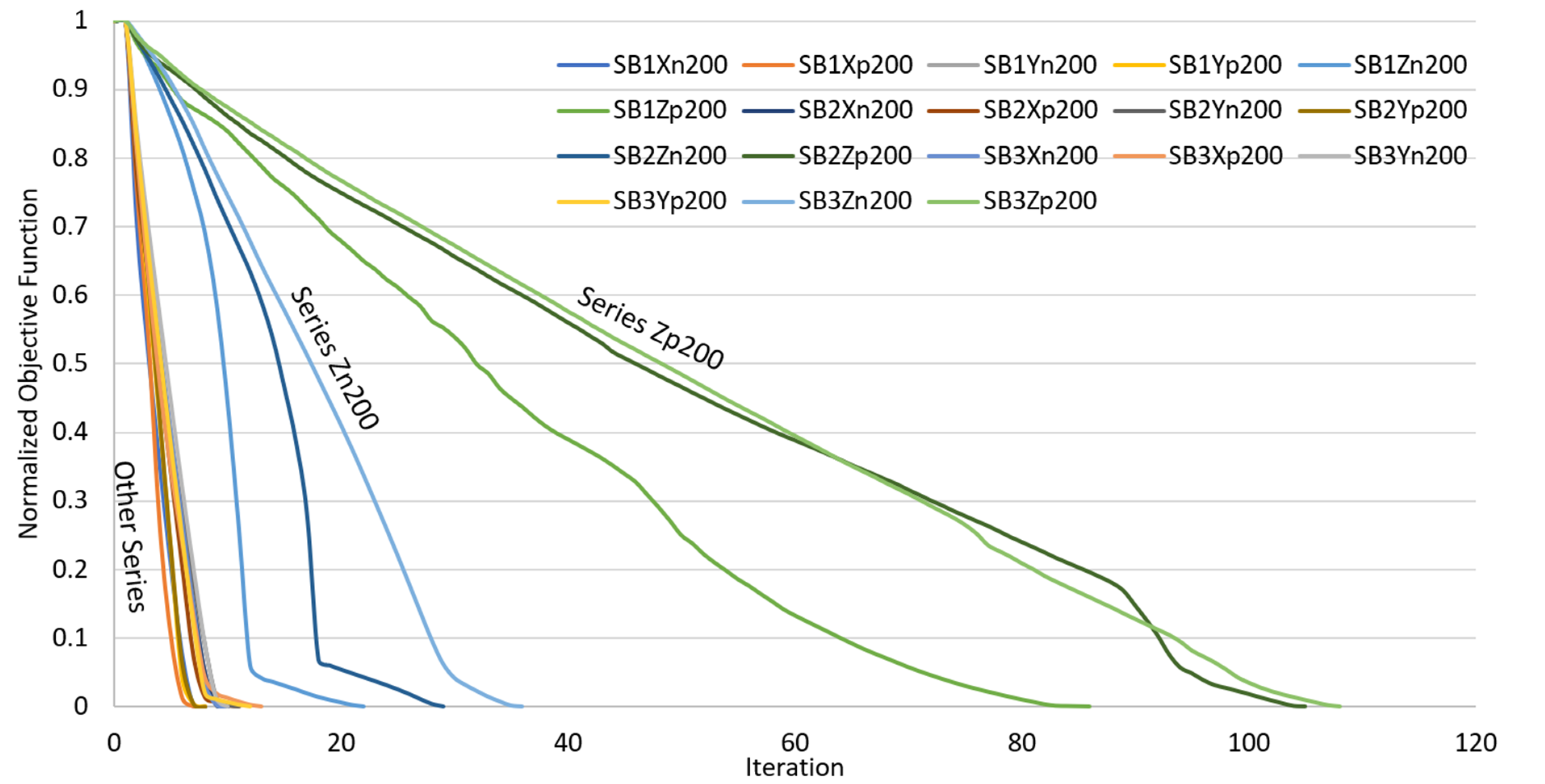
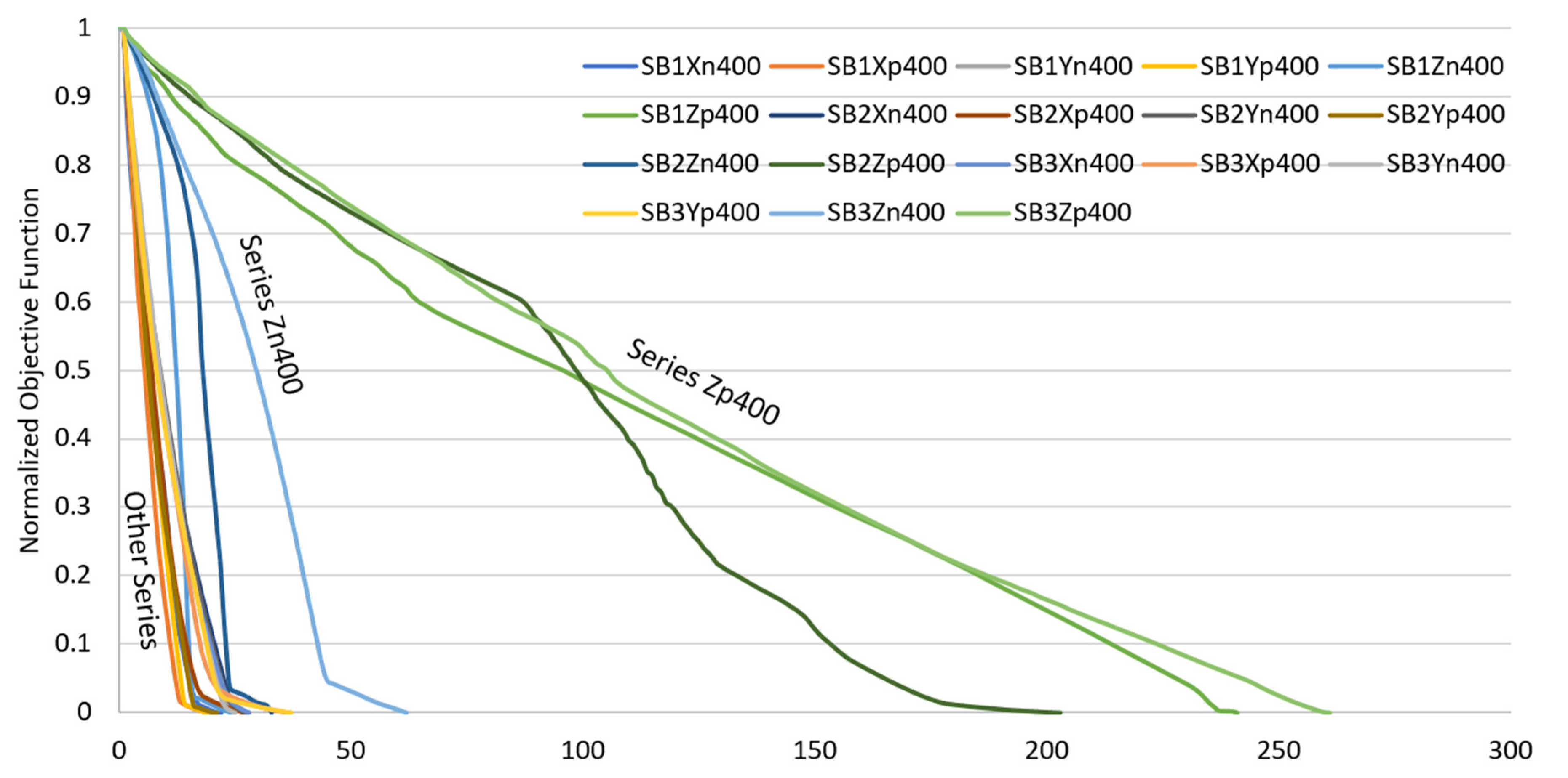
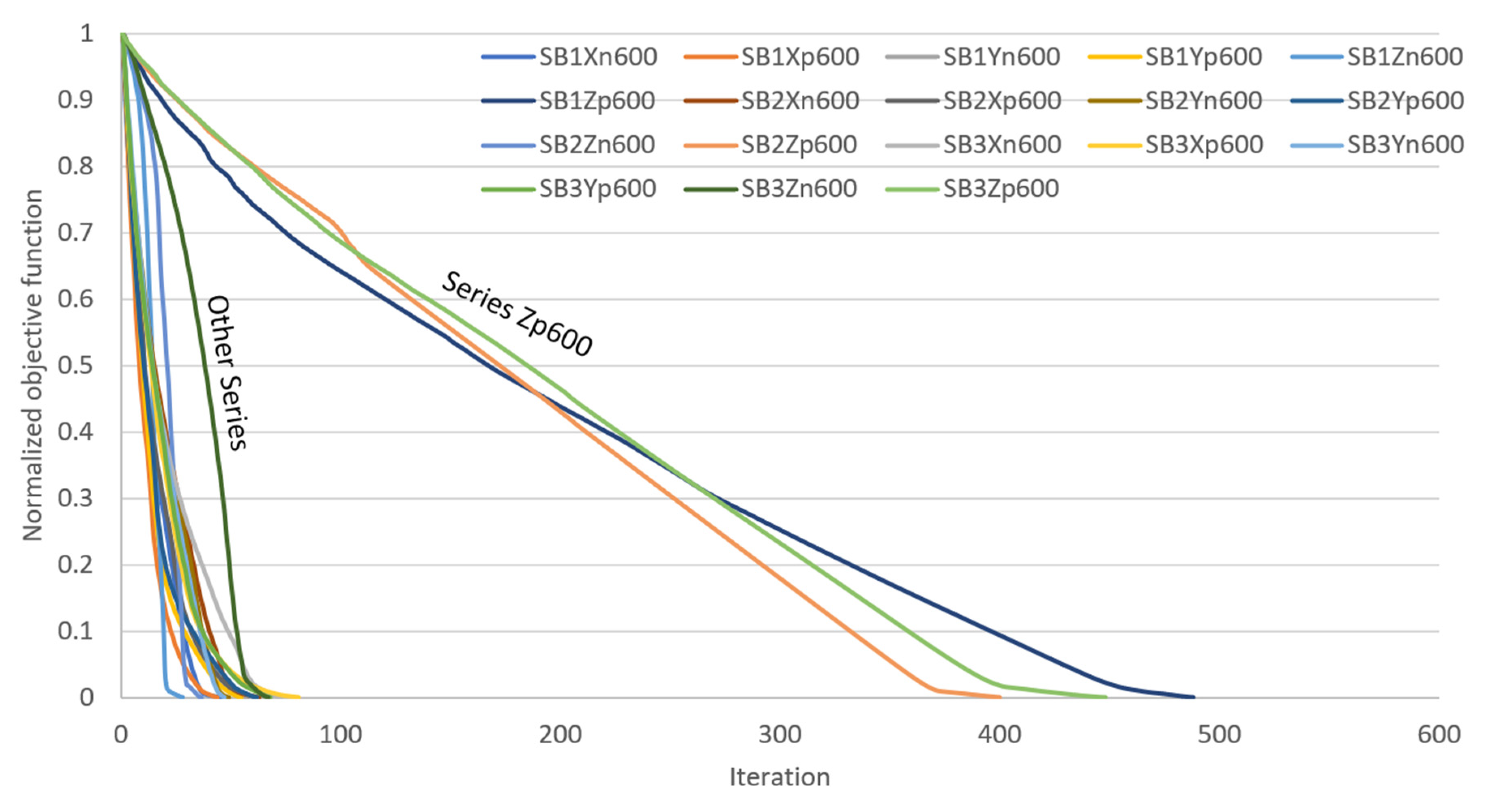
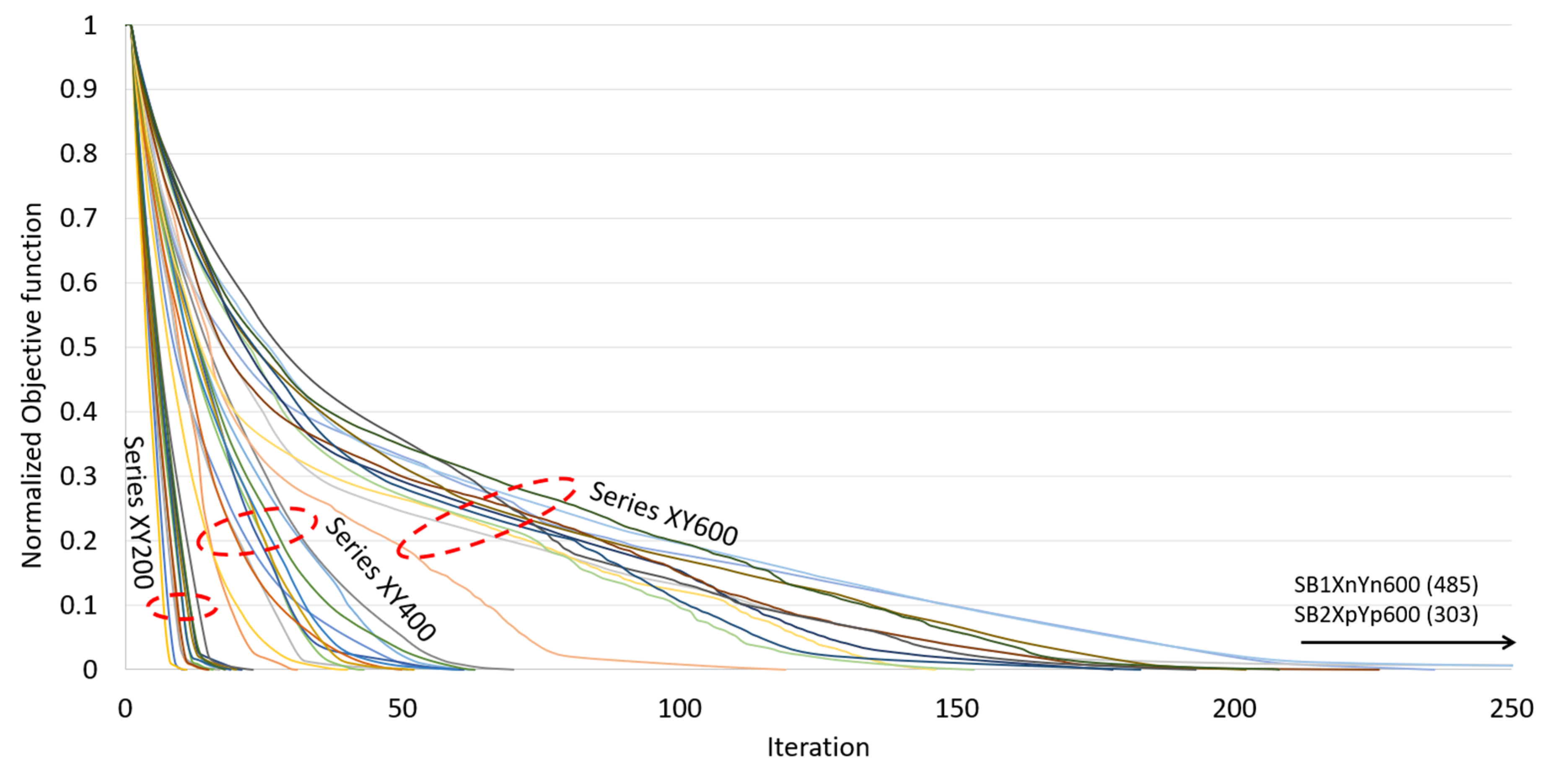
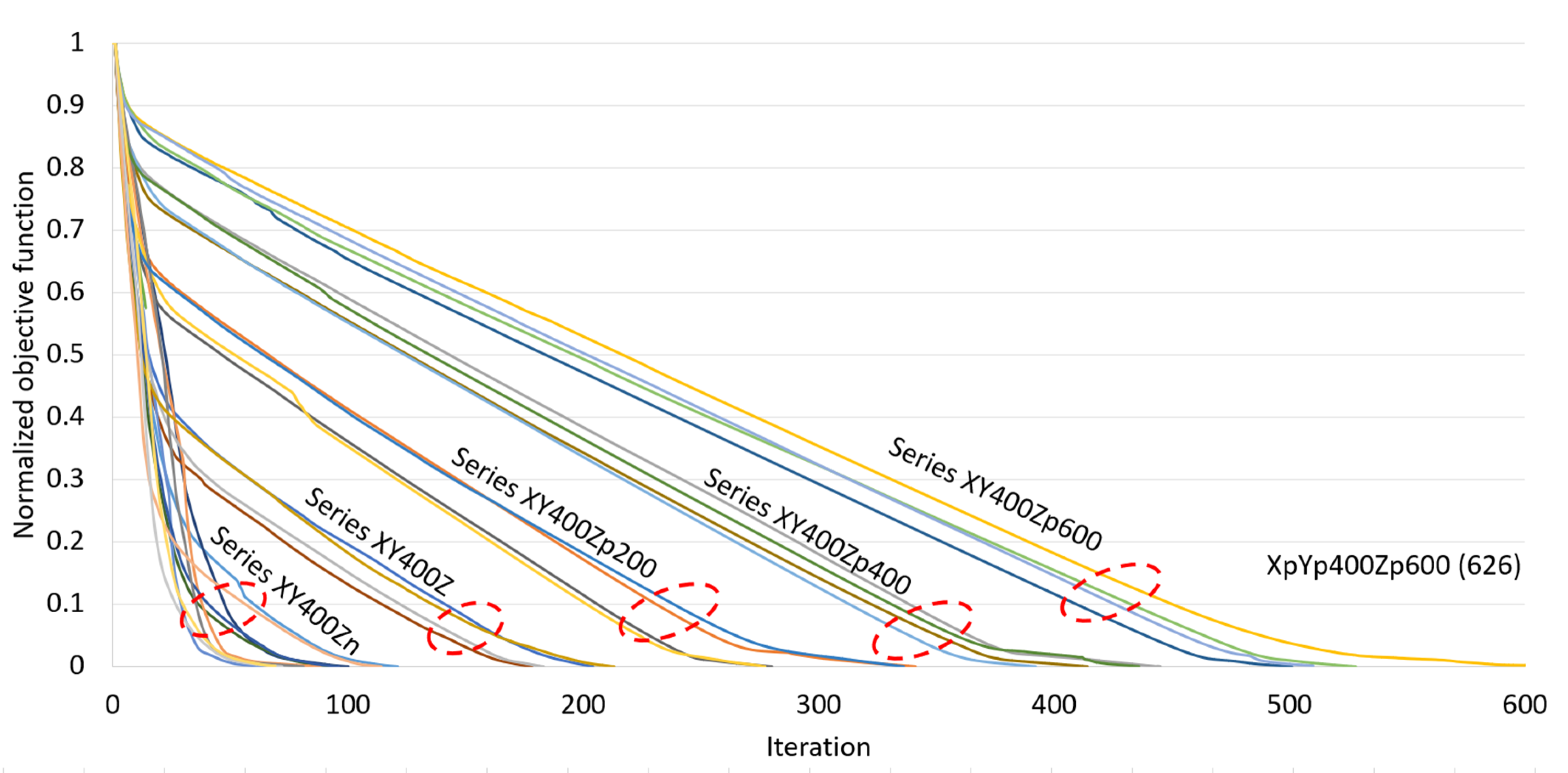
4.2. Convergence History

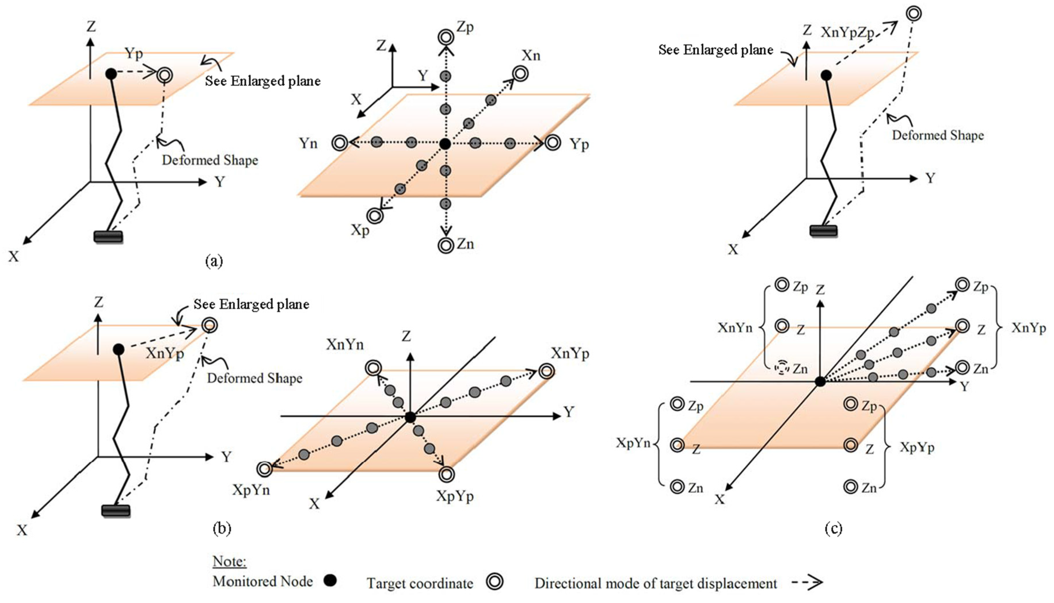
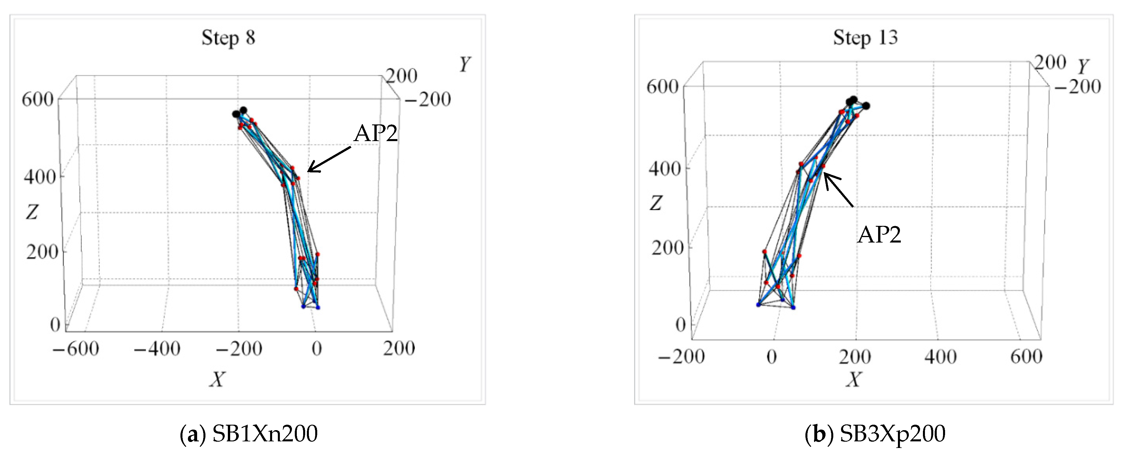
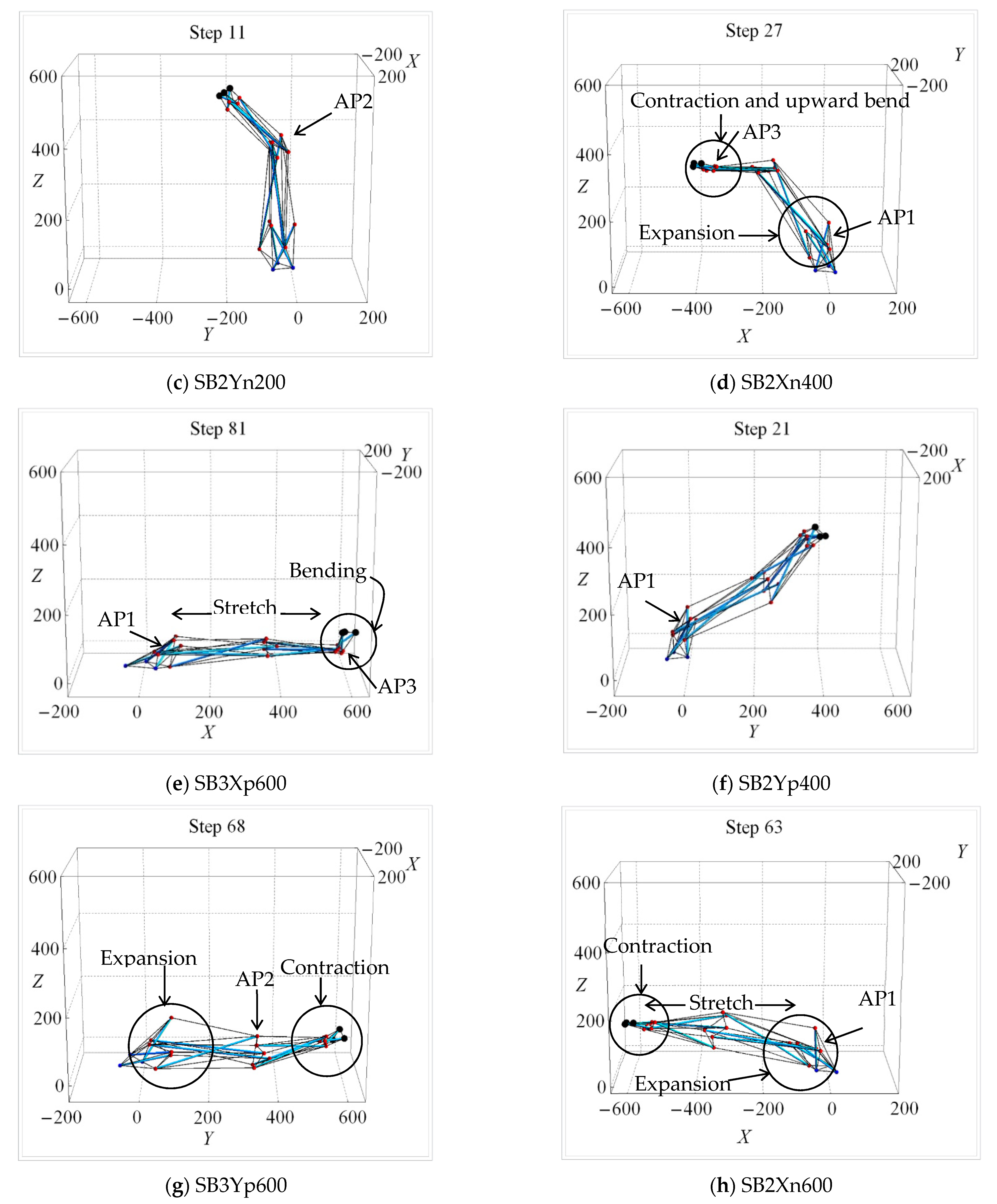
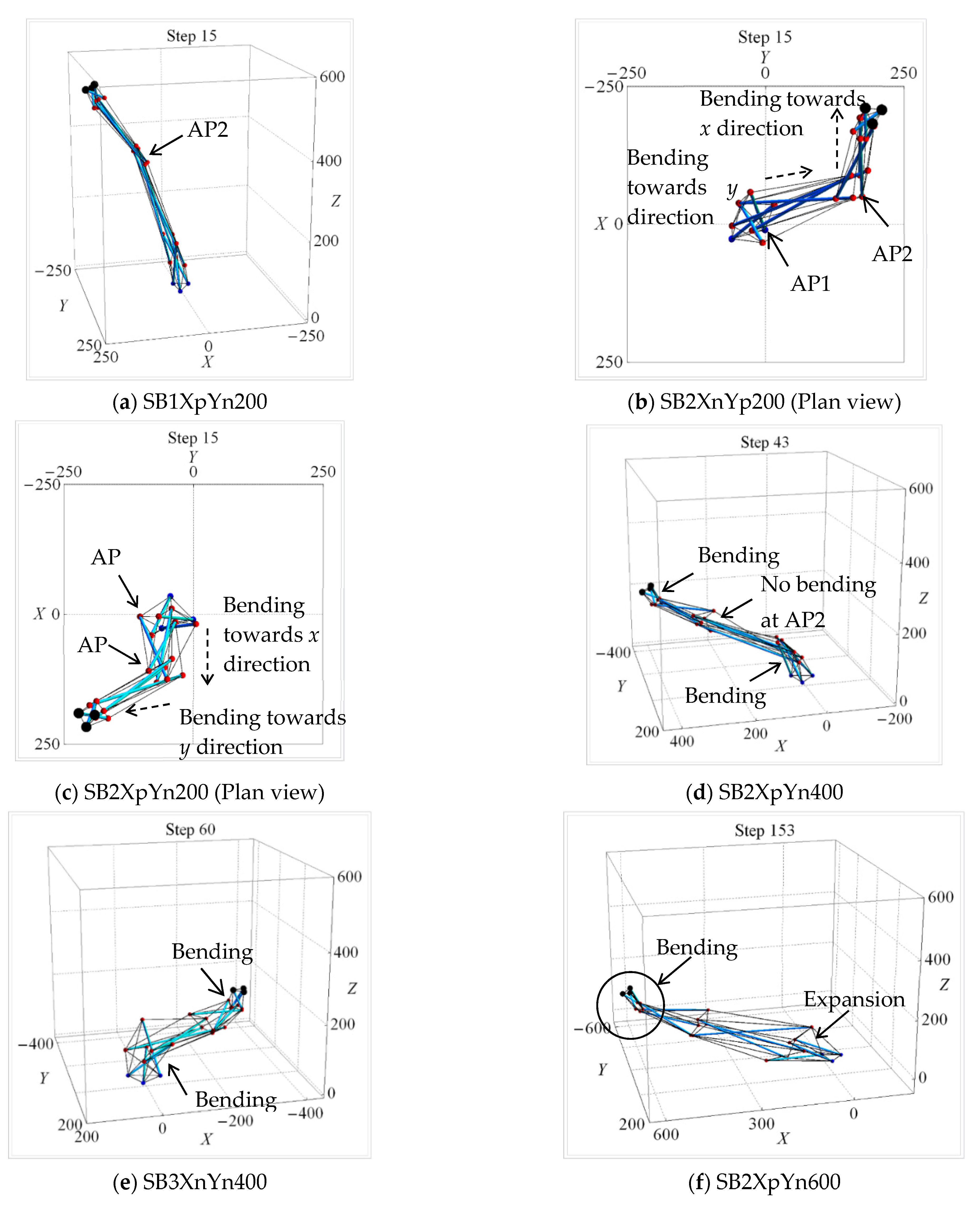
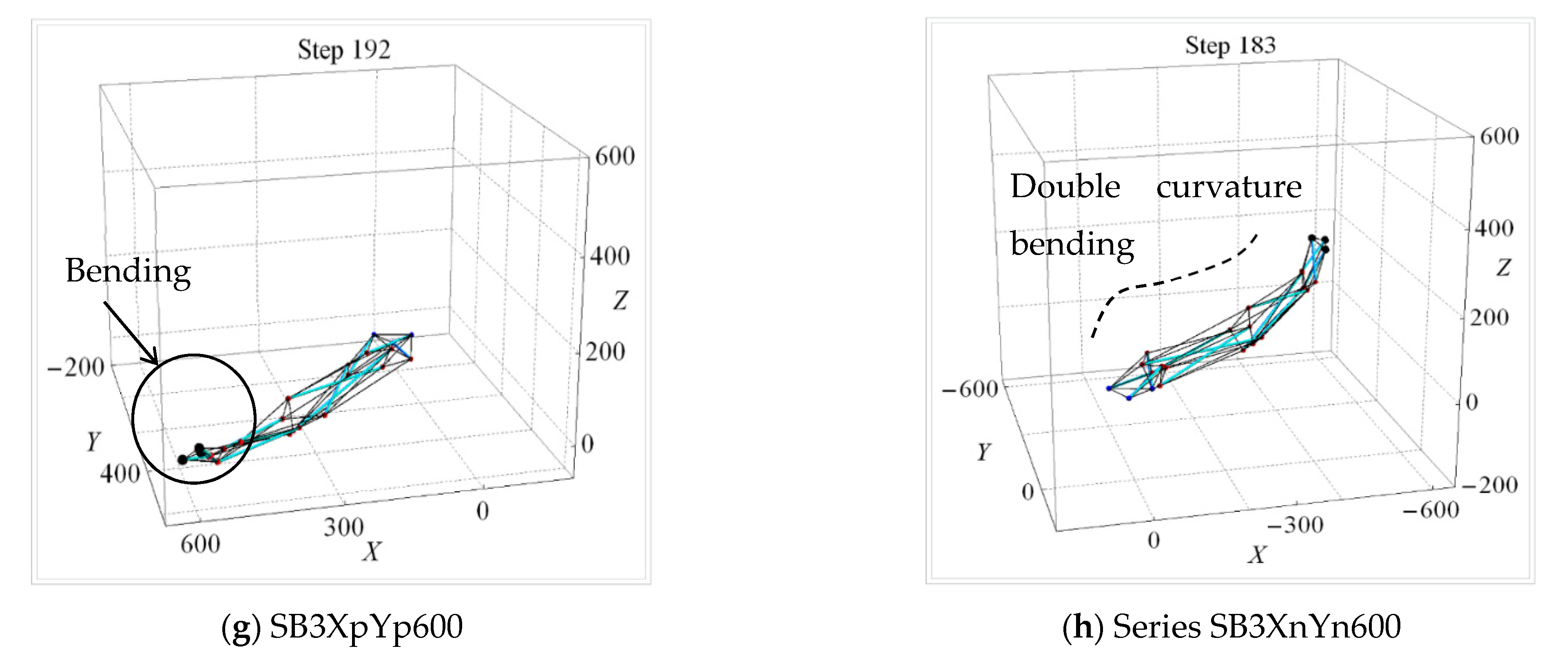
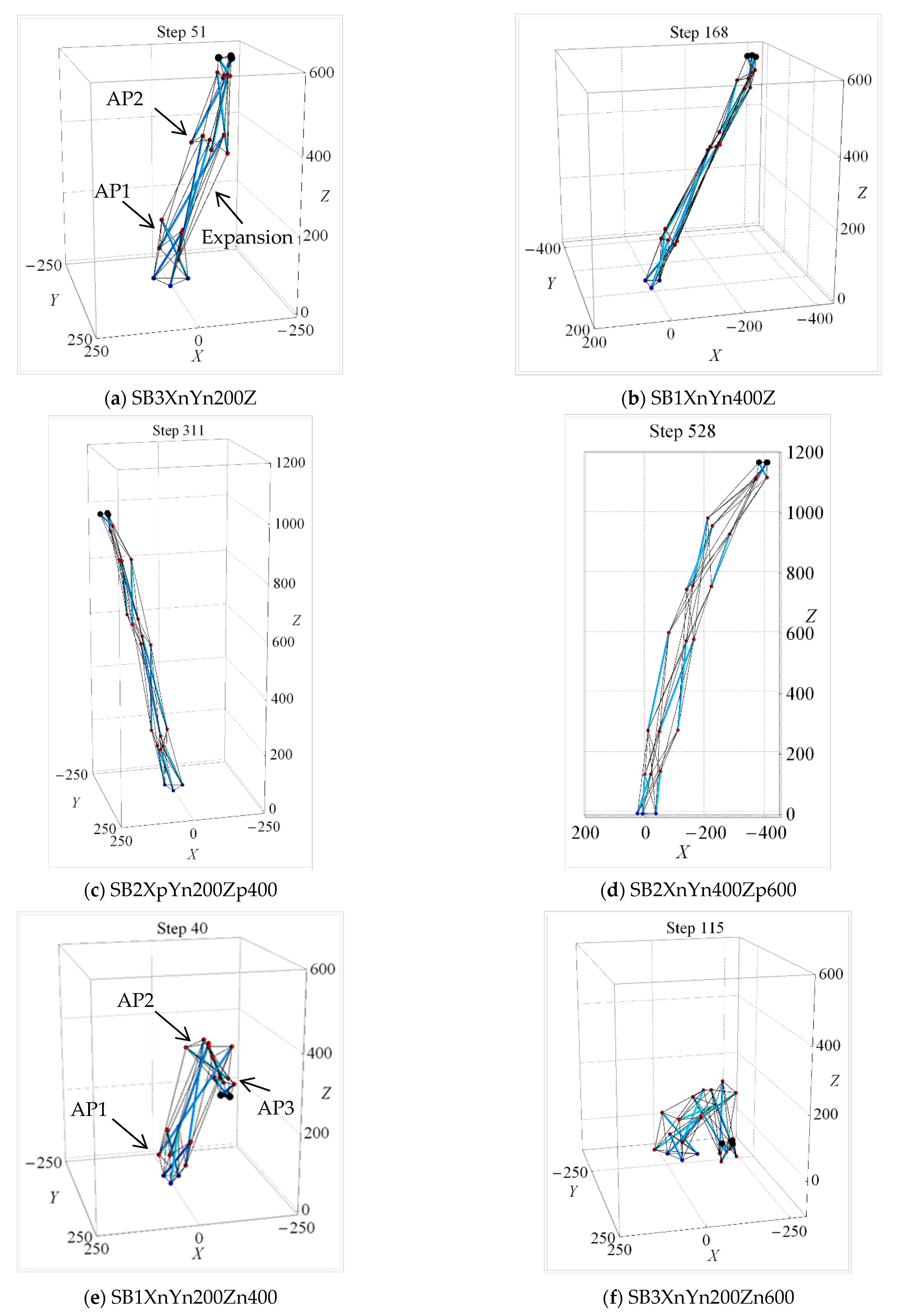
Figure 9, Figure 10 and Figure 11 show the plots of the normalized objective function (NOF) versus the iteration for 54 cases of shape change analysis with different target displacements in the uni-directional mode for SB1, SB2 and SB3 models. The NOF plots for all of the series show either linear or nonlinear patterns until reaching a plateau towards the end of the optimization process. Obvious differences in trends were noticed between the NOF plots for series Zp, Zn and the remaining series, particularly for cases with target displacements at 200 mm and 400 mm. For cases with target displacements of 600 mm, the pattern of plots for series Zp remains different from the others, while series Zn exhibits a similar NOF plot pattern to series Xn, Yp, Yn and Yp. Series Zp shows the highest iterations which are followed by series Zn and other series in most of the cases.

The slope of curves starts to change at an NOF lower than 0.05 in almost all of the cases. It is also clearly seen at an NOF lower than 0.05 that NOF plots of few analysis cases reach a plateau extending greater than a quarter of the total iteration (i.e., cases Xp400 and Yp400). Many applications such as inspections and maintenance works do not require high accuracy of the shape change results. Therefore, the efficiency of the proposed algorithm is rechecked by allowing a 2% error (where the value of 2% is based on the recorded successful rate of the overall analysis). It is found that, with this allowance, reduction of up to 40% total iteration in cases of target displacements in the uni-directional mode can be achieved.

Figure 12 shows the plots of the NOF versus iteration for 36 analysis cases with different target displacements in the bi-directional mode. The convergence of NOF in a nonlinear manner was observed in all of the cases with target displacements of 200 mm (series XY200), 400 mm (series XY400) and 600 mm (series XY600). A slower rate of convergence was generally observed at the end of the optimization process. Particularly, an unusual long plateau was observed in the analysis case SB1XnYn600 (up to 485 iterations), where the NOF of this case remained at the value of 0.01 for almost 60% of the total computational step. An allowance for a 2% error in the proposed algorithm can reduce up to 66% of the total computational step in analysis case SB1XnYn600 and up to 40% for the remaining cases of target displacements with the bi-directional mode.

Figure 13 and Figure 14 show the plots of the NOF versus iteration for 56 analysis cases with different target displacements in the tri-directional mode of SB2. Only the results of the analysis of model SB2 are shown, as similar trends of results are observed in the SB1 and SB3 models. The convergence of NOF in a nonlinear manner is observed in all of the cases in the tri-directional mode. There are also significant changes in slope observed in these NOF plots. For instance, series XY200Z and XY400Z show a significant change in slope at NOF of ranges of 0.1–0.3 and 0.3–0.5, respectively. The NOF in series Zp begins with a short and significant drop, which is then followed by a long curve with a linear decreasing pattern. Series XY200Zp and XY400Zp show a significant change in slope at NOF of ranges of 0.7–0.95 and 0.6–0.9, respectively. Generally, a more gradual slope in NOF is observed in series Zp compared to both series Z and Zn for all of the target displacement magnitudes of 200 mm, 400 mm and 600 mm. Series Zn only shows a change in slope at an NOF of less than 0.1 for all target displacements of 200, 400 and 600 mm.

Meanwhile, plateaus extending longer than half of the total computational steps (specifically at an NOF of less than 0.05) are clearly seen in 26 (13 for SB1, 9 for SB2 and 4 for SB3) out of 168 analysis cases with different target displacements in the tri-directional mode. Mainly, 13, 9 and 4 cases are identified for SB1, SB2 and SB3, respectively. The plateau in NOF plots for a few analysis cases even extends up to 80% of the total computational steps such as SB1XnYn200Zp600, SB1XnYp200Zp600 and SB2XpYn200Zp400 (see Figure 12). An allowance of a 2% error in the proposed algorithm eliminates the plateau in these two series and reduces up to 25% of the total computational steps, on average, for the remaining cases of target displacements under the tri-directional mode.

4.3. Deformed Modes

Figure 15 shows the deformed configurations at the final state for the selected cases in the uni-directional mode (series Xn, Xp, Yn and Yp). There are three apices in the spine biotensegrity models, namely, AP1, AP2 and AP3, which play a vital role as joints that permit bending. Generally, all of the spine biotensegrity models approach the target coordinates either by bending or by a combination of axial and bending deformations in cases of the uni-directional mode (i.e., series Xn, Xp, Yn and Yp). In these series, bending deformation primarily around AP2 was observed for a displacement of 200 mm (Figure 15a–c) and around all Aps (AP1 to AP3) for displacements of 400 mm and 600 mm (Figure 15d,e). However, due to the natural curvature in the YZ plane view, AP1 allows for greater bending compared to AP2 in most cases of series Yp (Figure 15f,g). Axial deformation accompanied by bending deformation was observed in most of the cases with a displacement of 600 mm, where the models bend about AP1 and AP3 while the segment between the two apices stretches (Figure 15g,h). Additionally, the deformation of spine biotensegrity models through expansion and contraction were observed (Figure 15d). The shape change analysis case Xp400 of SB2 can be found in Video S1: Shape Change of Biotensegrity Model Mimicking Human Spine in the Supplementary Materials section.

Figure 16 shows the final state for series Zn and Zp in cases of the uni-directional mode. Spine biotensegrity models in series Zn achieved the targets by means of bending or axial deformation or a combination of both. Conversely, spine biotensegrity models in series Zp exhibit solely axial deformation. In series Zn, SB1 and SB2 demonstrate bending deformation with obvious bending about AP2 (Figure 16a,b). The bending deformation is mainly towards the positive y-axis, with the thoracic kyphosis (refer to the initial configuration in Figure 3 and the deformed configuration at the final state in Figure 15b) falling on the opposite side. On the other hand, SB3 demonstrates bending deformation about two axes. Specifically, the segments between AP1 and AP2 demonstrate bending deformation about the y-axis, whereas bending about the x-axis was observed in the upper segments (Figure 16c,d). In series Zp, all of the spine biotensegrity models approach the target through the lengthening of cables resulting in axial deformation. It is noted that the spine biotensegrity models were stacked up with upper cell sunk into the lower cell, forming sag depth at all of the apices (Figure 3). At the initial state, the lower triangular surface of the upper cell (denoted as l.t. in Figure 16e–g) is located below the upper triangular surface (denoted as u.t. in Figure 16e–g). The height of l.t increased and gradually exceeded the height of u.t during the shape change analysis. Such height increment was demonstrated firstly at AP3 (Figure 16e), which is then followed by AP2 and later AP1 (Figure 16f,g), with the increase in target displacement magnitudes. Deformations in terms of contraction and expansion were also observed in both series Zn and Zp.

Figure 17 shows the final state for cases of the bi-directional mode. In cases with target displacement magnitude of 200 mm, all spine biotensegrity models approach the target coordinates by means of bending deformation, either about one axis (Figure 17a) or two axes (Figure 17b,c). For cases with target displacement magnitude of 400 mm, the spine biotensegrity models generally demonstrate bending deformation with slight axial deformation (Figure 17d,e). Displacements of AP1 and AP3, which resulted in bending deformations with double curvature, were observed. However, no significant bending was observed at the segments between AP1 and AP3. The deformation characteristics of all of the spine biotensegrity models except series XnYn were governed primarily by axial deformations at target displacement magnitude of 600 mm, accompanied by expansion and contraction. Along with the axial deformation, most of the spine biotensegrity models allow for slight bending around AP3 (Figure 17f,g). In a way different from the other series, series XnYn demonstrates double curvature bending deformation (Figure 17h). Despite the fact that monitored nodes are only prescribed at the top, the deformation of nodes at AP1 was clearly observed during the shape change process. Similar to the human spine, the struts (i.e., vertebrae) and cables (i.e., muscle) of the spine biotensegrity model act in an interrelated manner. The far-away members can act immediately when the signal was given even to local points to advance to a set of targets.

Figure 18 shows the final state for cases of shape change analysis involving the tri-directional mode. SB models in series XY200Z reach their target coordinates mainly by means of bending deformation about AP1 and AP2 (Figure 18a). On the contrary, almost all SB models in series XY400Z reach the target coordinates by means of axial deformation (Figure 18b). In series Zp, all SB models in series XY200Zp and XY400Zp reach the target coordinates by means of axial deformation (Figure 18c,d). The vertical clearance between the two groups of nodes (the upper and lower nodes) becomes significant when both x and y or z target displacement magnitudes increase.

On the other hand, all SB models in series XY200Zn reach the target coordinates primarily by means of bending deformation. In cases with z target displacement magnitude of 200 mm, all SB models in series XpYn and XnYn generally bend around AP2 whereas series XpYp and XnYp demonstrate noticeable bending around both AP1 and AP2. When the z target displacement magnitude increases, bending deformation around all apices, AP1, AP2 and AP3, is observed (Figure 18e). Bi-axial bending is also observed in most of the cases (Figure 18f), except series XnYn, which shows only uni-axial bending. Generally, the majority of all SB models in series XY400Zn show axial deformation with slight bending around AP3 in most of the cases with z-displacement magnitude of 200 mm, while, for cases of magnitudes of target displacement equal to 400 mm and 600 mm, bending around AP1 and AP2 is generally seen. It is noted that all SB models demonstrate expansion and contraction in the final configuration. The proposed spine model incorporates the freedom of movement inherent in humans but does not necessarily exhibit the same movements experienced by humans. Depending on the settings of the analysis model, it may show cases of shape change that exceed the limits of human spine movement, as shown in Figure 15, Figure 16, Figure 17 and Figure 18. Nevertheless, the findings derived from the use of the simplified spine biotensegrity model considered in this study provide useful insight into the influence of the incorporation of human spine topology on the deformation characteristics of the model.

5. Conclusions

This paper presented a shape change analysis of three variations of biotensegrity models inspired by the form of the human spine, SB1-3 in the cases of uni-, bi- and tri-directional modes. The formulation of incremental equilibrium equations and the exploitation of the optimization tool, particularly the sequential quadratic programming method, were presented. The proposed shape change algorithm is capable of simulating the shape change of spine biotensegrity models via four states, the initial state, the deformed state, the shape change state and the target state, which allows for the advancement of the monitored nodes to approach to the target coordinates. The algorithm successfully solves the nonlinear programming problem, searches for the optimized forced elongation for cables and ensures non-slackened cables during the shape change analysis under specific constraints. A highly successful rate (99.62%) in achieving the objective function was observed in a total of 54, 35 and 168 analysis cases dealing with uni- (99.96%), bi- (99.98%) and tri-directional modes (98.92%), respectively. The convergence results can be further enhanced after the allowance of relaxing tolerance of 2% in the algorithm.

Generally, no significant variation in the results of the total computational steps, NOF and displacement of the monitored nodes corresponding to the type of SB models was observed. The capability of the spine biotensegrity models to undergo bending and axial deformation and combinations of these deformations was proven in the study. The results of deformed configurations suggest that the spine biotensegrity models (SB1, SB2 and SB3) have more flexibility to undergo bending deformation in comparison with axial deformation. Apices (i.e., AP1, AP2 and AP3) in the spine biotensegrity models act as joints to permit the bending, extension, contraction and rotation in the shape change process. The contribution of the apices in shape change depends on the target displacement magnitude and the distance of the apice from the monitored nodes. Understanding the potential deformations of the spine biotensegrity models during the shape change process is essential for further extension to the simulation of shape change control. Towards the above mentioned direction, member and external obstacle collision avoidance, as well as the application of multiple series of monitored nodes, should be explored in future studies. Furthermore, the extension of the modeling of the human spine to incorporate parts connected to the spine, as well as more constraints on the movement of the human spine in the formulation of shape change analysis strategy, should also be considered.

References

1. Swanson, R.L. Biotensegrity: A Unifying Theory of Biological Architecture with Applications to Osteopathic Practice, Education, and Research—A Review and Analysis. J. Osteopat. Med. 2013, 113, 34–52. [Google Scholar] [CrossRef] [Green Version]
2. Bordoni, B.; Myers, T. A Review of the Theoretical Fascial Models: Biotensegrity, Fascintegrity, and Myofascial Chains. Cureus 2020, 12, e7092. [Google Scholar] [CrossRef] [PubMed] [Green Version]
3. Crowle, A.; Harley, C. Development of a biotensegrity focused therapy for the treatment of pelvic organ prolapse: A retrospective case series. J. Bodyw. Mov. Ther. 2020, 24, 115–125. [Google Scholar] [CrossRef] [PubMed]
4. Sharkey, J. Biotensegrity-Anatomy for the 21st Century Informing Yoga and Physiotherapy Concerning New Findings in Fascia Research. J. Yoga Physiother. 2018, 6, 1–4. [Google Scholar] [CrossRef]
5. Oh, C.L.; Choong, K.K.; Nishimura, T.; Kim, J.-Y. Form-finding of spine inspired biotensegrity model. Appl. Sci. 2020, 10, 6344. [Google Scholar] [CrossRef]
6. Kan, Z.; Peng, H.; Chen, B.; Zhong, W. Nonlinear dynamic and deployment analysis of clustered tensegrity structures using a positional formulation FEM. Compos. Struct. 2018, 187, 241–258. [Google Scholar] [CrossRef]
7. Kan, Z.; Peng, H.; Chen, B.; Zhong, W. A sliding cable element of multibody dynamics with application to nonlinear dynamic deployment analysis of clustered tensegrity. Int. J. Solids Struct. 2018, 130–131, 61–79. [Google Scholar] [CrossRef]
8. Zhu, D.; Deng, H. Deployment of tensegrities subjected to load-carrying stiffness constraints. Int. J. Solids Struct. 2020, 206, 224–235. [Google Scholar] [CrossRef]
9. Cai, H.; Wang, M.; Xu, X.; Luo, Y. A General Model for Both Shape Control and Locomotion Control of Tensegrity Systems. Front. Built Environ. 2020, 6, 98. [Google Scholar] [CrossRef]
10. Zhang, L.; Gao, Q.; Liu, Y.; Zhang, H. An efficient finite element formulation for nonlinear analysis of clustered tensegrity. Eng. Comput. 2016, 33, 252–273. [Google Scholar] [CrossRef]
11. Veuve, N.; Safaei, S.D.; Smith, I.F. Active control for mid-span connection of a deployable tensegrity footbridge. Eng. Struct. 2016, 112, 245–255. [Google Scholar] [CrossRef] [Green Version]
12. Yang, S.; Sultan, C. Deployment of foldable tensegrity-membrane systems via transition between tensegrity configurations and tensegrity-membrane configurations. Int. J. Solids Struct. 2019, 160, 103–119. [Google Scholar] [CrossRef]
13. Yıldız, K.; Lesieutre, G.A. Deployment of n-Strut Cylindrical Tensegrity Booms. J. Struct. Eng. 2020, 146, 04020247. [Google Scholar] [CrossRef]
14. Shintake, J.; Zappetti, D.; Peter, T.; Ikemoto, Y.; Floreano, D. Bio-inspired Tensegrity Fish Robot. In Proceedings of the 2020 IEEE International Conference on Robotics and Automation (ICRA), Paris, France, 31 May–31 August 2020; pp. 2887–2892. [Google Scholar]
15. Ramadoss, V.; Sagar, K.; Ikbal, M.S.; Calles, J.H.L.; Zoppi, M. HEDRA: A Bio-Inspired Modular Tensegrity Soft Robot with Polyhedral Parallel Modules. arXiv 2011, arXiv:142402020. [Google Scholar]
16. Wei, D.; Gao, T.; Mo, X.; Xi, R.; Zhou, C. Flexible Bio-tensegrity Manipulator with Multi-degree of Freedom and Variable Structure. Chin. J. Mech. Eng. 2020, 33, 3. [Google Scholar] [CrossRef] [Green Version]
17. Liu, S.; Li, Q.; Wang, P.; Guo, F. Kinematic and static analysis of a novel tensegrity robot. Mech. Mach. Theory 2020, 149, 103788. [Google Scholar] [CrossRef]
18. Oh, C.L.; Choong, K.K.; Nishimura, T.; Kim, J.-Y.; Hassanshahi, O. Shape change analysis of tensegrity models. Lat. Am. J. Solids Struct. 2019, 16, 1–19. [Google Scholar] [CrossRef] [Green Version]
19. Busscher, I.; Ploegmakers, J.J.W.; Verkerke, G.J.; Veldhuizen, A.G. Comparative anatomical dimensions of the complete human and porcine spine. Eur. Spine J. 2010, 19, 1104–1114. [Google Scholar] [CrossRef] [PubMed] [Green Version]
Figure 1. (a) Human spine anatomy (lateral view), and (b) typical vertebrae (superior and lateral views).
Applsci 12 02377 g001
Figure 2. Different sizes of typical triangular cells for spine biotensegrity models.
Applsci 12 02377 g002
Figure 3. Self-equilibrated configuration for spine biotensegrity models (a) SB1, (b) SB2 and (c) SB3 [5].
Applsci 12 02377 g003
Figure 4. Algorithm for shape change analysis.
Applsci 12 02377 g004
Figure 5. Cases of target displacements: (a) uni-directional; (b) bi-directional; and (c) tri-directional modes.
Applsci 12 02377 g005
Figure 6. Computational steps in series dealing under the uni-directional mode.
Applsci 12 02377 g006
Figure 7. Computational steps in series under bi-directional mode.
Applsci 12 02377 g007
Figure 8. Computational steps in series under tri-directional mode for SB2 model (left) series XY200 and (right) series XY400.
Applsci 12 02377 g008
Figure 9. Convergence history for 18 shape change analysis cases in the uni-directional mode with target displacement of 200 mm.
Applsci 12 02377 g009
Figure 10. Convergence history for 18 shape change analysis cases in the uni-directional mode with target displacement of 400 mm.
Applsci 12 02377 g010
Figure 11. Convergence history for 18 cases with the uni-directional mode with target displacement of 600 mm.
Applsci 12 02377 g011
Figure 12. Convergence history for 36 shape change analysis cases in the bi-directional mode for series XY200, XY400 and XY600.
Applsci 12 02377 g012
Figure 13. Convergence history for 28 shape change analysis cases in the tri-directional mode for series XY200 for SB2.
Applsci 12 02377 g013
Figure 14. Convergence history for 28 shape change analysis cases in the tri-directional mode for series XY400 for SB2.
Applsci 12 02377 g014
Figure 15. Deformed configuration (ah) at the final step for cases with the uni-directional mode, series Xn, Xp, Yn and Yp.
Applsci 12 02377 g015aApplsci 12 02377 g015b
Figure 16. Deformed configuration (ag) at the final step for cases with the uni-directional mode, series Zn and Zp.
Applsci 12 02377 g016aApplsci 12 02377 g016b
Figure 17. Deformed configuration (ah) at the final step for cases with the bi-directional mode.
Applsci 12 02377 g017aApplsci 12 02377 g017b
Figure 18. Deformed configuration (af) at the final step for cases with the tri-directional mode.
Applsci 12 02377 g018