An Adaptive Operational Modal Analysis under Non-White Noise Excitation Using Hybrid Neural Networks

Abstract

To adaptively identify the modal parameters for time-invariant structures excited by non-white noise, this paper proposes a new operational modal analysis (OMA) method using hybrid neural networks. In this work, taking the acceleration response directly as the input data of the networks not only simplifies the data processing, but also retains all the characteristics of the data. The data processed by the output function is the output data of the network, and its peak corresponds to the modal frequency. The proposed output function greatly reduces the computational cost. In addition, a small sample dataset ensures that the hybrid neural networks identify the modal parameters with the highest accuracy in the shortest possible time. Interestingly, the hybrid neural networks combine the advantages of the convolutional neural network (CNN) and gate recurrent unit (GRU). To illustrate the advantages of the proposed method, the cantilever beam and the rudder surface excited by white and non-white noise are taken as examples for experimental verification. The results reveal that the proposed method has a strong anti-noise ability and high recognition accuracy, and is not limited by ambient excitation type.

1. Introduction

OMA is a process of identifying structural modal parameters only according to the response, including time-domain or frequency-domain techniques. It is well known that modal characteristics can be used in various structural health monitoring applications [1,2,3]. As such, modal analysis plays a key role in many engineering applications [4,5,6].

Recently, various methods for identifying modal parameters of time-invariant structures were proposed [7,8,9,10]. Additionally, the simplest and most typical one is the peak picking (PP) method [11]. In addition, the frequency-domain decomposition technique that has been widely studied by researchers [12,13,14,15] is constantly being improved; for instance, the enhanced frequency-domain decomposition (EFDD) algorithm can predict not only the natural frequencies, but also estimate modal damping ratios [16]. Further, the frequency and spatial domain decomposition (FSDD) technique was one of the most successful modifications of the classical frequency-domain decomposition, it was a more sensitive modal damping estimation method [17]. Compared with the frequency-domain method, the time-domain method can obtain the system parameters directly from the response signal. Thus stochastic subspace identification (SSI), autoregressive moving average time series analysis methods, and their improved methods have been widely used in engineering practice [18,19,20]. The methods based on random decrement technology, the Ibrahim time-domain method, natural excitation technology, eigensystem realization algorithm, and other technologies are also powerful modal analysis tools for time-invariant structures [21,22,23,24]. In addition, the least-squares complex exponential method, Hilbert–Huang transform, and their improved methods appear one after another [25,26,27]. Given the abundant literature for OMA, it is noticeable that most of the traditional OMA methods only identify the time-invariant structures excited by white noise [28]. However, in reality, many ambient excitations are not compliant with the white noise assumption [29]. Researchers began to study the OMA method excited by non-white noise. For instance, an OMA method based on the response correlation function for rotating structures is proposed [30]. In addition to the approaches above, the modal parameters of structures can be identified in another way by a neural network. The neural network algorithm can approach any function in theory, has a strong nonlinear mapping ability, and the adaptability of the network is strong [31].

As the profound research of neural networks, the method of neural network was successfully used in many fields, for instance, optimization, signal processing, health monitoring, and fault diagnosis [32,33,34]. In Ref. [35], a random CNN was proposed to extract signals automatically through convolution operation to monitor the working conditions of the diesel engine. Moreover, Yu et al. proposed a residual neural network based on the characteristic of vibration signal [36]. In Ref. [37], the improved fault diagnosis method based on CNN is proposed, which used a light neural network to process the original signal. The above methods and their application in practical engineering owing to the ability of the neural networks extract signal characteristics. Due to the unique advantages of neural networks in data mining and feature extraction [38,39], the OMA method based on the network came into being. For instance, the three support vector regression method using observed vibration data was proposed [40]. In Ref. [41], the OMA method based on the back propagation network was also proposed. With the development of deep learning, a method based on an uncertainty diagram and CNN was proposed [42]. The research of the OMA method using neural networks is valuable and has a bright future. The universal approximation theorem proposed by Cybenko [43] shows that a simple neural network can approach the expected function infinitely, given appropriate parameters. However, the training optimization algorithm is not necessarily able to learn the function. In many cases, using a deeper model can reduce the number of units required and reduce the generalization error. Nevertheless, the large amount of sample data increases the characteristic parameters of the model, resulting in a long training time, with an unstable model training effect.

To handle these concerns, a hybrid neural network based on CNN and GRU is proposed. Taking advantage of CNNs and GRU, the hybrid neural network can extract features from a long sequence with small sample data to reduce the computational cost. In hybrid neural networks, firstly, the CNN with strong feature extraction ability is used to preliminarily extract features, and then the preliminarily extracted feature information is fed into GRU for deeper learning. It can reduce the network characteristic parameters and network layers, to achieve the purpose of short training time and fast convergence speed. The rest of this work is structured as follows. First, the background is detailed in Section 2. Second, the method and simulation verification is provided in Section 3. Then, the experimental verification is provided in Section 4. Finally, conclusions are described in Section 5.

2. Background

2.1. Operational Modal Analysis

In a linear N degree of freedom system, the relationship between the response and excitation of the power spectral density (PSD) matrices can be expressed as

$${\mathit{S}}_{yy}(j\omega )={\mathit{H}}^{*}(j\omega ){\mathit{S}}_{xx}(j\omega ){\mathit{H}}^{\mathrm{T}}(j\omega ),$$

(1)

where S_yy and S_xx are the response and excitation PSD matrices, respectively. ‘*’ is the conjugacy of the matrix, and ‘T’ denotes the transposition operation. Additionally, H(jω) is the frequency response function (FRF) matrix:

$$\mathit{H}(j\omega )={\displaystyle \sum _{r=1}^N\left[\frac{{\mathit{R}}_r}{j\omega -s_r}+\frac{{\mathit{R}}_r^{*}}{j\omega -s_r^{*}}\right]},$$

(2)

$${\mathit{R}}_r={\mathit{\varphi }}_r{\mathit{\gamma }}_r^{\mathrm{T}},$$

(3)

where s_r = −p_r + j q_r is the rth pole, p_r q_r is the damping factor, and q_r is the damped modal frequency. Additionally, R_r is the residue, ϕ_r is the modal shape, and γ_r is the modal participation vector. According to Equations (1) and (2):

$${\mathit{S}}_{yy}(j\omega )={\displaystyle \sum _{r=1}^N\left[\frac{{\mathit{A}}_r}{j\omega -s_r}+\frac{{\mathit{A}}_r^{\mathrm{H}}}{-j\omega -s_r^{*}}+\frac{{\mathit{A}}_r^{*}}{j\omega -s_r^{*}}+\frac{{\mathit{A}}_r^{\mathrm{T}}}{-j\omega -s_r}\right]},$$

(4)

$${\mathit{A}}_r={\displaystyle \sum _{b=1}^N\left[\frac{{\mathit{R}}_b^{*}{\mathit{S}}_{xx}{\mathit{R}}_r^{\mathrm{T}}}{-s_b^{*}-s_r}+\frac{{\mathit{R}}_b{\mathit{S}}_{xx}{\mathit{R}}_r^{\mathrm{T}}}{-s_b-s_r}\right]}.$$

(5)

In general, the damping of structure is small. Suppose that s_r = −p_r + j q_r is satisfied with p_r « q_r, A_r ≈ d_rφ_r^*φ_r^T, and d_r is a real number.

$${\mathit{S}}_{yy}(j\omega )\approx {\displaystyle \sum _{r=1}^N\left[\frac{d_r{\mathit{\varphi }}_r^{*}{\mathit{\varphi }}_r^{\mathrm{T}}}{j\omega -s_r}+\frac{d_r{\mathit{\varphi }}_r^{*}{\mathit{\varphi }}_r^{\mathrm{T}}}{-j\omega -s_r^{*}}\right]}={\mathit{\psi }}^{*}\mathrm{diag}[2\mathrm{Re}(\frac{d_r}{j\omega -s_r})]{\mathit{\psi }}^{\mathrm{T}},\hspace{1em}\omega \to {\omega }_r,$$

(6)

$${\mathit{S}}_{yy}^{\mathrm{T}}(j\omega )\approx \mathit{\psi }\mathrm{diag}[2\mathrm{Re}(\frac{d_r}{j\omega -s_r})]{\mathit{\psi }}^{\mathrm{H}},\hspace{1em}\omega \to {\omega }_r,$$

(7)

The response PSD matrix can be decomposed by singular value decomposition (SVD) as

$${\mathit{S}}_{yy}^{\mathrm{T}}(j\omega )=\mathit{U}\mathit{\Lambda }{\mathit{U}}^{\mathrm{H}},$$

(8)

$$\mathit{\Lambda }=\mathrm{diag}({\lambda }_1,{\lambda }_2,\cdots ,{\lambda }_N),$$

(9)

where the superscript ‘H’ denotes the conjugate transposition operation, U ∈ C^Q×N is a unitary matrix, which contains singular vectors, and it corresponds to Ψ in Equation (7). Λ ∈ R^N×N is the diagonal matrix, which is composed of real singular values. Only the dominant modes are analyzed, and the rth mode of enhanced PSD can be expressed as

$${\mathit{P}}_{sd}(j\omega )={\mathit{U}}_r^{\mathrm{H}}{\mathit{S}}_{yy}^{\mathrm{T}}(j\omega ){\mathit{U}}_r.$$

(10)

On the near spectral line, the enhanced PSD function is made of the singular value of the response spectrum matrix corresponding to U_r.

$$P_{sd}(j\omega )\approx 2\mathrm{R}\mathrm{e}(\frac{d_r}{\mathrm{j}\omega -s_r})$$

(11)

Substitute s_r into Equation (11), so the enhanced PSD function can be written as:

$$\mathit{B}\left[\begin{array}{c}{\mathit{P}}_{sd}\\ \omega {\mathit{P}}_{sd}\\ 1\end{array}\right]=-{\omega }^2{\mathit{P}}_{sd},$$

(12)

$$\mathit{B}=\left[\begin{array}{ccc}{p}_r^2+q_r^2& -2q_r& -2d_r{p}_r\end{array}\right],$$

(13)

Understandably, the response signal contains all the required modal information. Then, the least-squares solution of row vector B is obtained by giving ω_i in the range of interest, and then the corresponding modal frequencies and damping are obtained.

$$f_r=\sqrt{p_r^2+q_r^2},$$

(14)

$${\zeta }_r=\frac{p_r}{\sqrt{p_r^2+q_r^2}}=\frac{p_r}{f_r}.$$

(15)

The derivation of the above equations are the assumption that the input is a flat spectrum (white noise excitation). However, in many actual cases, the ambient excitation is non-white noise [29,30]. For this reason, a general output function is proposed, which is no longer limited to the assumption of white noise excitation, and its peak point corresponds to each order of modal frequency.

$$\mathit{O}\left(f_f\right)={\displaystyle \sum _{h=1}^{N_r}\exp [-{\left(f_f-F_h\right)}^2]},$$

(16)

where F_h denotes the frequency of the hth peak of the singular value curve, N_r takes order in this paper. For the output function, the find peaks function is used to identify the frequency of each order.

$$f^p={\mathrm{F}}_{\mathrm{P}}(\mathit{O}(f_f)),$$

(17)

where F_P(x) means looking for the peak of data, so we can directly read the modal frequencies of each order. Additionally, the output function is only related to the peak point of the singular value curve, which greatly reduces the computational cost, and is suitable for mixed noise excitation. The modal shape Ψ in Equation (7) corresponds to the singular value vector U in Equation (8), so the modal shape can be obtained according to the corresponding left singular value vector. Based on f^p, damping can be obtained according to Equations (11)–(15). The rth damping can be written as:

$${\stackrel{⌢}{\zeta }}_r=\frac{p_r}{f_r^p}.$$

(18)

2.2. CNN

Deep neural networks, such as CNN, have shown outstanding data modeling capabilities in various applications [44].

In the simplest case of the convolution layer,

$${\mathbf{Y}}_{\mathrm{C}}(N_i,C_{\mathrm{o}\mathrm{u}\mathrm{t} j})=b(C_{\mathrm{o}\mathrm{u}\mathrm{t} j})+{\displaystyle \sum _{k=0}^{C_{in}-1}w(C_{\mathrm{o}\mathrm{u}\mathrm{t} j},k)}*{\mathbf{X}}_C(N_i,k),$$

(19)

where the superscript ‘*’ denotes valid cross-correlation operations, N represents the batch size, and C denotes channel. C_in and C_out are the input and output channels in the convolution layer, respectively. X_C and Y_C are the input and output data in the convolution layer, respectively. b is the bias and w is the weight.

The addition of the pooling layer to the convolution layer can decrease the dimension of the feature map to decrease the parameters that are finally transported to the fully connected layer, thereby speeding up the operation speed and avoiding overfitting.

In the sampling layer,

$${\mathrm{Y}}_P(N_i,C_j,k)=\underset{0,\cdots ,m-1}{\mathrm{m}\mathrm{a}\mathrm{x}}{\mathrm{X}}_P(N_i,C_j,s\times k+m),$$

(20)

where X_P and Y_P are the input and output data in the sampling layer, respectively. m and s express the kernel size and the stride, respectively.

2.3. GRU

Unlike the long short-term memory network (LSTM) [45], GRU only has an update gate and reset gate. Therefore, it has few parameters and good convergence. The forward propagation of GRU is as follows,

$$r_t^G=\sigma (W_{ir}{x}_t^G+b_{ir}+W_{hr}{h}_{t-1}^G+b_{hr}),$$

(21)

$$z_t^G=\sigma (W_{iz}{x}_t^G+b_{iz}+W_{hz}{h}_{t-1}^G+b_{hz}),$$

(22)

$$n_t^G=\mathrm{t}\mathrm{a}\mathrm{n}\mathrm{h}(W_{in}{x}_t^G+b_{in}+W_{hn}{h}_{t-1}^G+b_{hn}),$$

(23)

$$h_t^G=(1-z_t^G)\odot n_t^G+z_t^G\odot h_{t-1}^G,$$

(24)

$$y_t^G=\sigma (W_o\times h_t^G+b_o),$$

(25)

where $h_t^G$ represents the hidden state at time t, X_G = [$x_1^G$, $x_2^G$, …, $x_t^G$,…] and Y_G = [ $y_1^G$, $y_2^G$, …, $y_t^G$,…] are the input and output data, respectively. $r_t^G$, $z_t^G$, $n_t^G$ express the reset gate, update gate, and new gate, respectively. σ denotes the sigmoid function, and ‘⊙’ denotes the Hadamard product operation.

In the process of network transmission, the loss of a single sample is as follows:

$$E_t=\frac{1}{2}{(y_t^G-{\widehat{y}}_t^G)}^2,$$

(26)

$$E={\displaystyle {\sum }_{t=1}^T{E}_t}.$$

(27)

The input–output relationship of the back propagation algorithm [46] network is essentially a highly nonlinear mapping relationship. The back propagation process of the GRU are shown in Equations (28)–(34).

$$\frac{\partial E}{\partial W_o}={\delta }_{y,t}{h}_t^G,$$

(28)

$$\frac{\partial E}{\partial W_{iz}}={\delta }_{z,t}{x}_t^G,$$

(29)

$$\frac{\partial E}{\partial W_{hz}}={\delta }_{z,t}{h}_{t-1}^G,$$

(30)

$$\frac{\partial E}{\partial W_{in}}={\delta }_t{x}_t^G,$$

(31)

$$\frac{\partial E}{\partial W_{ih}}={\delta }_t(r_t^G\times h_{t-1}^G),$$

(32)

$$\frac{\partial E}{\partial W_{ir}}={\delta }_{r,t}{x}_t^G,$$

(33)

$$\frac{\partial E}{\partial W_{hr}}={\delta }_{r,t}{h}_{t-1}^G,$$

(34)

where

$${\delta }_{y,t}=(y_t^G-{\widehat{y}}_t^G)\times {\sigma }^{\prime },$$

(35)

$${\delta }_{h,t}={\delta }_{y,t}{W}_o+{\delta }_{z,t+1}{\mathrm{W}}_{\mathrm{h}\mathrm{z}}+{\mathrm{\delta }}_{\mathrm{t}+1}{W}_{hn}\times r_{t+1}^G+{\delta }_{h,t+1}{W}_{hr}+{\delta }_{h,t+1}\times (1-z_{t+1}^G),$$

(36)

$${\delta }_{z,t}={\delta }_{t,h}\times (n_t^G-h_{t-1}^G)\times {\sigma }^{\prime },$$

(37)

$${\delta }_t={\delta }_{h,t}\times z_t\times {\varphi }^{\prime },$$

(38)

$${\delta }_{r,t}=h_{t-1}^G\times [({\delta }_{h,t}\times z_t^G\times {\varphi }^{\prime })W_{hn}]\times {\sigma }^{\prime },$$

(39)

Update the parameters and iterate successively until the loss converges.

3. The Proposed Method and Simulation Verification

3.1. Dataset Process

The cantilever beam is used as the structural model to simulate the slender aerospace structure [29], and the ambient excitation of the structure is simulated by base excitation. The beam is shown in Figure 1, which is divided into 10 elements. Generally, the damping ratio of the actual aluminum beam is 0.01–0.03, so the damping ratio of the beam is 0.01 in the simulation. In practical engineering, the system is not constant, such as a rocket launch. With the consumption of fuel, the mass of the system decreases continuously [47]. Therefore, 11 beams with different masses are constructed for the simulation. Take the first beam as a reference; the mass change of the other 10 beams are (0.001; 0.002; 0.003; 0.004; 0.005; 0.006; 0.007; 0.008; 0.009; and 0.01) kg. Therefore, the mass change of the first beam and the 11th beam is 0.01 kg. The mass change is located on the 10th node of the 10th unit of the beam, and the others are the same. The length is 0.8 m, the section height is 0.012 m, and the width is 0.06 m. The elastic modulus is 7.1 × 10¹⁰ Pa, and the mass density is 2770 kg/m³. In addition, the spectral lines is 1600 and the analysis frequency band is 1000 Hz.

The construction process of the dataset is as follows. Taking the response directly as the input data of the network not only simplifies the data processing process, but also retains all the characteristics of the data. The noise with different signal-to-noise ratios (SNRs) [48] is added to the acceleration response. Additionally, the acceleration response signal is then processed according to the O (f_f) (Section 2.1) to obtain the output data of the network (Figure 2). More specifically, each beam has 500 samples for model training. Therefore, the dataset is composed of 500 × 11 samples, and each sample represents a two-dimensional matrix.

3.2. The Proposed Method

Initially, the features of the acceleration response are extracted by the CNN, as shown in Section 2.2. Additionally, the Mish function [49] is used in the convolution layer because of its remarkable accuracy and generalization ability.

$$\mathrm{t}\mathrm{a}\mathrm{n}\mathrm{h}(x_x)=\frac{e^{x_x}-e^{-x_x}}{e^{x_x}+e^{-x_x}},$$

(40)

$$\mathrm{M}(x_x)=x_x\times \mathrm{t}\mathrm{a}\mathrm{n}\mathrm{h}[\mathrm{l}\mathrm{n}(1+e^{x_x})],$$

(41)

$${\mathbf{Y}}_{P(i,j,k)}=\mathrm{m}\mathrm{a}\mathrm{x}(\mathrm{M}(b_j+{\displaystyle \sum _{k=0}^{C_{in}-1}{w}_{jk}}*{\mathrm{R}}_{ik})).$$

(42)

Here, the loss function of the whole network structure is the mean square error (MSE).

$$\mathrm{M}\mathrm{S}\mathrm{E}=\frac{1}{n}{\displaystyle \sum _{i=1}^n{(y_i-{\widehat{y}}_i)}^2},$$

(43)

where n denotes the total number, y_i and ŷ_i are the actual and the predicted output value, respectively.

In the second step, GRU is used to learn the features extracted by CNN.

$${\mathit{Y}}_G=\mathrm{G}({\mathit{Y}}_P),$$

(44)

where G (·) denotes the GRU networks calculation, and it is detailed in Section 2.3. Y_P is both the output of CNN and the input of GRU networks, and Y_G is the output of GRU networks.

Finally, the learned features are infinitely approximated to the final output of the network through the activation function.

$$y_i=\mathrm{P}\mathrm{R}\mathrm{e}\mathrm{L}\mathrm{U}(x_i{w}_i+b_i),$$

(45)

The PReLU [50] function has the characteristics of fast convergence and simple gradient calculation, and it is the activation function of the fully connected layer.

$$\mathrm{P}\mathrm{R}\mathrm{e}\mathrm{L}\mathrm{U}(x_x)=\{\begin{array}{cc}{x}_x& x_x\ge 0\\ a{x}_x& \mathrm{o}\mathrm{t}\mathrm{h}\mathrm{e}\mathrm{r}\mathrm{s}\end{array}.$$

(46)

In brief, the hybrid neural network consists of the convolutional layer, the max-pooling layer, the GRU layer, and the fully connected layer (Figure 3 and

Table 1. Parameters of the hybrid neural network.

Layer	Parameters	Activation Function
Conv1 (C1)	kernel size = 64; stride = 1; padding = 2; input channels = 1; output channels = 16	Mish
Max pooling1 (P1)	data kernel size = 2; stride = 2	-
GRU (G2)	hidden size = 256; layers = 2	tanh
Fully connected layer3 (FC3)	Inputdim = Size(YG); Outputdim = Size (Output)	PReLU

). For convenience, the capitalized initials of each layer are used to represent the corresponding network layer. The model first uses the convolutional layer C1 to learn features and then uses the Mish function to map the feature nonlinearly, where A1 is obtained. Next, the pooling layer P1 is applied to down-sample the features in A1. Then, the features in P1 are flattened into a vector and it is inputted into layer G2 for deep learning through GRU. Finally, the output is calculated through the full connection layer FC3.

Understandably, the more training set data, the better the parameters of the fitting curve can be determined, which is more conducive to the final optimization and determination of the model. On the contrary, the more test set data, the more accurate the generalization error estimation of the model. Therefore, trade-offs need to be made when dividing the dataset. The dataset is divided based on the hold-out method. Generally, about 2/3~4/5 samples are used for training. The most common training set and test set proportions are 6:4, 7:3, or 8:2. As mentioned earlier, the data sets with different proportions of training sets (50%, 60%, 70%, 80%, and 90%) are trained and tested many times, and the average value is taken for comparison. It is found that the more training set data, the longer the training time, and the training time is 203 s~292 s. The tested root mean square errors (RMSEs) were 1.89%, 0.96%, 0.64%, 0.21%, and 0.26%, respectively. When the training set data accounts for 80% and 90%, the test RMSE is better, but the training time of 90% data is 292 s more than that of 80% data, which is 246 s. As mentioned earlier, we investigated the selection of the percentage of the training samples and finally determined that the training sample percentage is 80%. Additionally, we investigated the impact of batch size on the comprehensive ability of the model, and finally determined that the batch size is 64.

To prove the advantages of the hybrid neural network, when different network structures train the same dataset, the advantage of the proposed method is self-evident, as in Figure 4. More specifically, when the proposed method reaches the fifth iteration, the value of the loss function is close to the optimal, and the curve is smoother than other network structures, indicating that this structure has the best training effect and the fastest convergence speed. As expected, the training times of CNN and LSTM are the longest and shortest, respectively. The training time of the proposed method and GRU is similar to that of LSTM. Interestingly, the training time of the proposed method is far less than the sum of the training times of CNN and GRU, indicating that the proposed method perfectly inherits the advantages of CNN and GRU. In addition, according to Equations (47)–(49), the test MRE and MARE of the proposed method is the smallest, indicating that the performance of this structure is the strongest. The comprehensive evaluation shows that the proposed method is the best.

$$\mathrm{R}\mathrm{E}=y_i-{\widehat{y}}_i$$

(47)

$$\mathrm{M}\mathrm{R}\mathrm{E}=\max (\mathrm{R}\mathrm{E})=\underset{i\in (1,n)}{\max }(y_i-{\widehat{y}}_i)$$

(48)

$$\mathrm{M}\mathrm{A}\mathrm{R}\mathrm{E}=\frac{1}{n}{\displaystyle \sum _{i=1}^n(\mathrm{R}\mathrm{E})}=\frac{1}{n}{\displaystyle \sum _{i=1}^n(y_i-{\widehat{y}}_i)}$$

(49)

3.3. Modal Training and Results

The response data with different SNRs are trained to test the proposed method’s anti-noise ability. The response data without SNR accounts for 40%, and others are 20%, respectively. The proposed method first trains the dataset and then tests the first beam. As shown in Figure 5a, 11 beams with different SNRs are trained. When iterating to step 5, four loss function curves are close to the optimal and reach the optimal in step 10, and these loss function curves are smooth, indicating that the model training effect is good. Then, the first beam with different SNRs is tested. As shown in Figure 5b, the test results have peaks at the same position, and the first five modal frequencies (15 Hz; 95.63 Hz; 268.8 Hz; 526.9 Hz; and 871.3 Hz) are obtained according to Equation (17). The convergence rate during training is the same, and the test results are the same, indicating that the noise cannot affect the network training and test results, so the proposed method’s anti-noise ability is strong. Furthermore, by comparing the analytical solution, the finite element solution, and the test results of the first beam (Figure 5b), it is found that the test results are consistent with other solutions, which verifies the effectiveness of the proposed method (Figure 6). The modal shapes conform to reality (Figure 7).

4. Experimental Verification

To verify the proposed method, a slender aluminum beam and an aluminum rudder surface structure were selected as the experimental specimens.

4.1. Dataset

Along the Y direction marked in Figure 8, the shaker table presents a base excitation. The experimental parameters are shown in

Table 2. Experimental parameters.

Physical Parameters		Experimental Parameters
Elastic Modulus (Pa)	Mass Density (kg/m3)	Spectral Lines	Analysis Frequency Band (Hz)	Sampling Frequency (Hz)	Sampling Length (s)	Test Time (s)
7.1 × 1010	2770	800	1000	2560	0.8	400

. The Agilent VXI Plus&Play system is acceleration signal acquisition equipment. The sensitivity of the acceleration sensor is 100.4 mv/g, and the type is PCB 333B32. In the experimental system of the slender aluminum beam, the first five acceleration sensors measure the acceleration response signals, including white noise and non-white noise excitations, and the last sensor measures the excitation signals (Figure 8). In the experimental system of the aluminum rudder space structure, the first acceleration sensor measures the white noise and non-white noise excitation signals, and the second and third sensors measure the acceleration response signals (Figure 9).

In general, the white noise excitation spectrum refers to the excitation spectrum of PSD uniformly distributed throughout the frequency domain, and its PSD function is a straight line. The non-uniform excitation spectrum refers to the excitation spectrum of the PSD function is not a straight line, it is also called the non-white noise excitation spectrum. Within a given frequency range, blue noise, pink noise, purple noise, and brown noise (four typical non-white noises) refer to the increase and decrease in PSD by 3 dB and 6 dB per octave with the increase in frequency. The beam and rudder surface are widely used in the aerospace field and can be used to study the flight state of the aircraft, and the actual situation is non-white noise excitation [51]. In addition, the measurement of boundary layer pressure fluctuation in hypersonic wind tunnels shows that the boundary pressure fluctuation has a non-flat spectrum and should be regarded as non-white noise [52]. Therefore, three excitation spectra, including white and non-white noise excitations, are applied to simulate the ambient excitation in this paper. Where the excitation spectrum 1 is white noise excitation, the excitation spectrum 2 is a mixed spectrum composed of blue, narrow-band white, and pink noises. Similarly, excitation spectrum 3 is a mixed spectrum composed of purple, narrow-band white, and brown noises (Figure 10).

As mentioned earlier, according to the dataset construction process (Figure 2), the response signals measured under the above three spectrum excitations (Figure 10) are processed, and the dataset is constructed. The dataset obtained by processing the acceleration response signals of the beam (Figure 8b) excited by excitation spectrum 1 are regarded as dataset 1, and the dataset obtained by processing the acceleration response signals of the beam excited by excitation spectrum2 and excitation spectrum 3 are regarded as dataset 2. Similarly, the dataset obtained by processing the acceleration response signals of the rudder surface (Figure 9b) excited by excitation spectrum 1 are regarded as dataset 3, and the dataset obtained by processing the acceleration response signals of the rudder surface excited by excitation spectrum2 and excitation spectrum 3 are regarded as dataset 4. The training set and test set proportion are 8:2.

4.2. Conventional OMA Methods

The conventional OMA methods, such as EFDD, FSDD, data-driven SSI (SSI-DATA), and covariance-driven SSI (SSI-COV), are used to identify the modal parameters of the beam (Figure 8b) under white noise (Figure 11) and non-white noise excitations (Figure 12 and Figure 13). However, as shown in Figure 12c, the SSI-COV method has first-order modal leakage in identifying the natural frequency of the beam excited by excitation spectrum 2. As shown in Figure 12d and Figure 13d, the SSI-DATA method also has first-order modal leakage in identifying the natural frequencies of the beam excited by excitation spectra 2 and 3. Additionally, according to Figure 13a–c, the EFDD, FSDD, and SSI-COV methods have mode leakages at the first natural frequency and false modes at the second natural frequency when identifying the modal frequency of the beam excited by excitation spectrum 3. Normally, the result of modal parameter identification excited by excitation spectrum 1 is considered to be accurate [21]. The analysis of Figure 11a,b and Figure 12a,b, shows that the EFDD and FSDD methods have no modal leakages and false modes when identifying the natural frequencies of the beam excited by excitation spectrum 2, but they are inconsistent with the identification results excited by excitation spectrum 1. More specifically, the first five natural frequencies of the beam under white (excitation spectrum 1) and non-white noise excitation (excitation spectrum 2) identified by EFDD are (16.83, 96.17, 306.41, 622.40, 997.5) Hz and (16.26, 97.42, 308.91, 619.90, 987.51) Hz, respectively, and the first five natural frequencies of the beam under white (excitation spectrum 1) and non-white noise excitation (excitation spectrum 2) identified by FSDD are (16.83, 97.46, 316.25, 617.75, 996.3) Hz and (16.83, 97.8, 311.0, 618.4, 1011.5) Hz, respectively. Briefly, different methods have different identification results for the same beam under a different excitation, the same method has different identification results for the same beam under a different excitation, and different methods have different identification results for the same beam under the same excitation.

4.3. Model Training and Results

Firstly, the dataset is substituted into the proposed model for training with the iteration steps is 50, and the learning rate is 0.001. The training process and test results are represented in Figure 14 below. The optimal value is reached in the first 10 steps, and the iterative curve is smooth, which shows that the model has a strong convergence ability (Figure 14a,b). Secondly, the network output is consistent with the target output and the proposed method has no modal leakage, showing that the network has high recognition accuracy. Finally, the test results of a different dataset of the beam are the same, and the training time is the same, indicating that the proposed method is not limited by the type of excitation signal (Figure 14c,d).

Experimental modal analysis is a method of parameter identification based on the measured excitation and response signals of the structure under laboratory conditions. Additionally, the results obtained by the experimental modal analysis are reliable, which is called analysis results.

The first five modal frequencies, (16.25 97.5 307.5 617.5 996.3) Hz, of the beam are obtained according to Equation (17). Based on the analysis results (Figure 15a), the relative error of identifying the modal frequency of the beam under non-white noise excitation by different methods is obtained, which is shown in

Table 3. The error of different methods for identifying the beam.

Methods		The Proposed Method	PP	EFDD	FSDD	SSI-COV	SSI-DATA
Excitation spectrum 1 (%)	1st	0	7.63	3.56	3.56	8.73	3.56
	2nd	0	−1.84	−1.36	−0.41	−1.26	4.41
	3rd	0	−0.06	−0.35	2.8	1.7	0.68
	4th	−0.21	0.18	0.58	−0.17	0.23	0.50
	5th	0	0.31	0.12	0	0.08	−1.27
Excitation spectrum 2 (%)	1st	0	−1.05	0.06	3.56	-	-
	2nd	0	0.82	−0.08	0.31	0.69	7.11
	3rd	0	0.94	0.46	1.14	0.62	1.09
	4th	−0.21	0.21	0.18	−0.065	0.036	0
	5th	0	0.37	−0.88	1.53	−0.14	−0.52
Excitation spectrum 3 (%)	1st	0	-	-	-	-	-
	2nd	0	1.39	−0.08	0.21	−2.84	10.2
	3rd	0	1.72	0.87	1.69	1.06	1.51
	4th	−0.21	1.26	0.18	0.15	0.23	0.21
	5th	0	0.37	1.01	2.02	−0.05	−0.37

. The recognition accuracy of the results of the proposed method is the highest, and the results under white and non-white noises excitation are consistent. Therefore, the proposed method can be used for non-white noise excitation, and it has strong anti-noise ability and strong applicability. According to Equation (47), error = (results obtained—analysis results)/analysis results × 100%.

Similarly, the proposed method is used to train and test the rudder surface. The optimal value is reached in the first 15 steps, which shows that the model has a strong convergence ability (Figure 16a,b). The test results of a different dataset of the rudder surface are the same, and the training time is the same, indicating that the proposed method is also applicable to other structures and has research value (Figure 16c,d). Frequency is an important characterization parameter for damage identification, health monitoring, and finite element analysis [1,5]. Therefore, accurate identification frequency has a high application value.

Based on the analysis results (Figure 15b), the relative errors of the proposed method under white and non-white noises excitation are analyzed, as in

Table 4. The relative error of the proposed method for identifying the rudder surface.

Excitations	The Proposed Method
	1st	2nd	3rd	4th
Excitation spectrum 1 (%)	0.19	0.04	0.049	−0.049
Excitation spectra 2 and 3 (%)	0.19	0.04	0.049	−0.049

. The results of the proposed method for identifying the rudder surface under different noise excitation are consistent, which shows that the anti-noise interference ability of the method is strong, and it is not limited to the excitation type. Compared with the analysis results, the identification errors of the first four frequencies are all less than 0.2%, so the proposed method has high identification accuracy.

5. Conclusions

An adaptive OMA method using a hybrid neural network is proposed and applied to extract modes from the acceleration response signals under non-white excitation. In this work, the proposed method has fewer layers and greatly fewer characteristic parameters, which simplifies the model and reduces the time cost of training and testing. The small sample dataset makes it possible to achieve the highest accuracy in the shortest possible time. The output function proposed in this paper is only related to the peak point of the singular value curve, which greatly reduces the computational cost, and can be used for non-white noise excitation.

(1)

According to the comparison of the training and test results of the same dataset with different network structures, it shows that the hybrid neural network is optimal.

(2)

A total of 11 beams with different qualities are numerically simulated. The training time and convergence speed of the response data with different SNRs are the same, and the test results of the first beam are the same, showing that the anti-noise ability of the proposed method is strong. In addition, the effectiveness of the method is proved by comparing with the finite element solution, analytical solution, and the test results of the first beam.

(3)

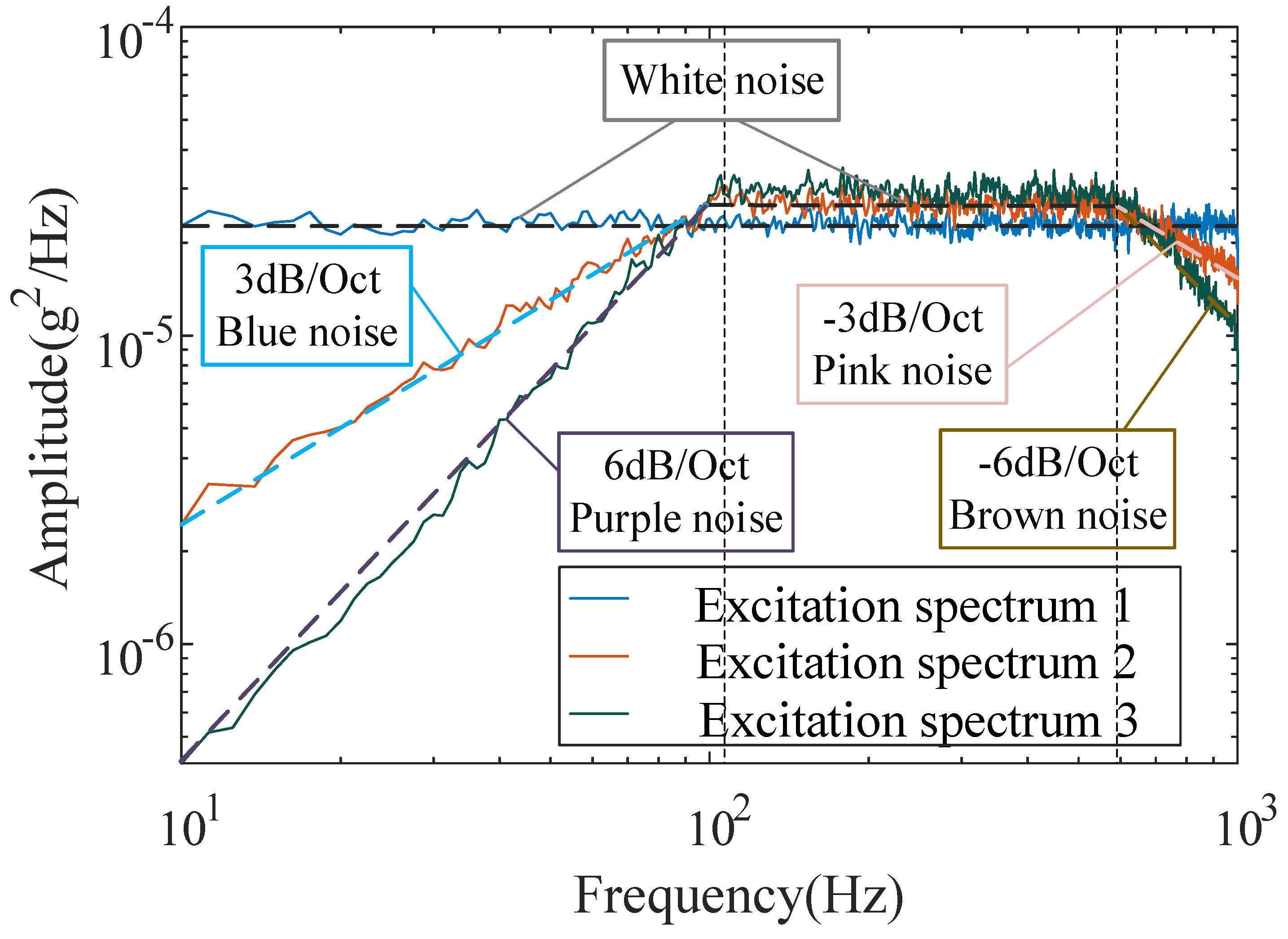
The conventional OMA methods are used to identify the modal parameters of the beam. There are false modes and mode leakage when identifying the modal parameters of the response under non-white noise excitation (excitation spectrum 2 and excitation spectrum 3). Taking the analysis results as a reference, the results of different methods for identifying the response under non-white noise excitation are compared. It is found that the proposed method has no modal leakage and the highest identification accuracy. Therefore, the proposed method is not limited by the excitation type and is more suitable for the actual ambient excitation.

(4)

The results of the proposed method for identifying the rudder surface under different noise excitations are consistent, which shows that the anti-noise ability of the method is strong. Compared with the analysis results, the identification errors of the first four modal frequencies are all less than 0.2%, so the identification accuracy of the proposed method is high.

References

1. Dong, X.; Man, J.; Wang, H. Structural vibration monitoring and operational modal analysis of offshore wind turbine structure. Ocean Eng. 2018, 150, 280–297. [Google Scholar] [CrossRef]
2. Ni, Y.C.; Alamdari, M.M.; Ye, X.W. Fast operational modal analysis of a single-tower cable-stayed bridge by a Bayesian method. Measurement 2021, 174, 109048. [Google Scholar] [CrossRef]
3. Pioldi, F.; Rizzi, E. Earthquake-induced structural response output-only identification by two different operational modal analysis techniques. Earthq. Eng. Struct. Dyn. 2018, 47, 257–264. [Google Scholar] [CrossRef]
4. Sun, Q.; Yan, W.J.; Ren, W.X. Application of transmissibility measurements to operational modal analysis of railway, highway, and pedestrian cable-stayed bridges. Measurement 2019, 148, 106880. [Google Scholar] [CrossRef]
5. Ebrahimi, R.; Mirdamadi, H.R.; Ziaei, R.S. Operational modal analysis and fatigue life estimation of a chisel plow arm under soil-induced random excitations. Measurement 2018, 116, 451–457. [Google Scholar] [CrossRef]
6. Xu, Y.F.; Chen, D.M.; Zhu, W.D. Operational modal analysis using lifted continuously scanning laser doppler vibrometer measurements and its application to baseline-free structural damage identification. J. Vib. Control 2019, 25, 1341–1364. [Google Scholar] [CrossRef]
7. Yanez-Borjas, J.J.; Amezquita-Sanchez, J.P.; Valtierra-Rodriguez, M.; Camarena-Martinez, D. Nonlinear mode decomposition-based methodology for modal parameters identification of civil structures using ambient vibrations. Meas. Sci. Technol. 2019, 31, 015007. [Google Scholar] [CrossRef]
8. Eitner, M.; Sirohi, J.; Tinney, C.E. Modal parameter estimation of a reduced-scale rocket nozzle using blind source separation. Meas. Sci. Technol. 2019, 30, 095401. [Google Scholar] [CrossRef]
9. Brincker, R.; Zhang, L.; Andersen, P. Modal identification from ambient responses using frequency domain decomposition. In Proceedings of the IMAC 18: Proceedings of the International Modal Analysis Conference (IMAC), San Antonio, TX, USA, 7–10 February 2000; pp. 625–630. [Google Scholar]
10. Auweraer, H.; Guillaume, P.; Verboven, P. Application of a fast-stabilizing frequency domain parameter estimation method. J. Dyn. Syst. 2001, 123, 651–658. [Google Scholar] [CrossRef]
11. Tomaszewska, A.; Drozdowska, M.; Szafrański, M. Material Parameters Identification of Historic Lighthouse Based on Operational Modal Analysis. Materials 2020, 13, 3814. [Google Scholar] [CrossRef]
12. Zimmerman, A.T.; Lynch, J.P. Market-based frequency domain decomposition for automated mode shape estimation in wireless sensor network. Struct. Control Health Monit. 2010, 17, 808–824. [Google Scholar] [CrossRef] [Green Version]
13. Ozer, E.; Purasinghe, R.; Feng, M.Q. Multi-output modal identification of landmark suspension bridges with distributed smartphone data: Golden Gate Bridge. Struct. Control Health Monit. 2020, 27, e2576. [Google Scholar] [CrossRef]
14. Amador, S.; Brincker, R. Robust Multi-dataset Identification with Frequency Domain Decomposition. J. Sound Vib. 2021, 508, 116207. [Google Scholar] [CrossRef]
15. Nita, G.M.; Mahgoub, M.A.; Sharyatpanahi, S.G.; Cretu, N.C.; El-Fouly, T.M. Higher order statistical frequency domain decomposition for operational modal analysis. Mech. Syst. Signal Process. 2017, 84, 100–112. [Google Scholar] [CrossRef]
16. Brincker, R.; Ventura, C.E.; Andersen, P. Damping estimation by frequency domain decomposition. In Proceedings of the International Modal Analysis Conference 19: A Conference on Structural Dynamics, Kissimmee, FL, USA, 5–8 February 2001; Volume 1, pp. 698–703. [Google Scholar]
17. Zhang, L.M.; Wang, T.; Tamura, Y. A frequency-spatial domain decomposition (FSDD) method for operational modal analysis. Mech. Syst. Signal Process. 2010, 24, 1227–1239. [Google Scholar] [CrossRef]
18. Zhou, Y.; Jiang, X.; Zhang, M. Modal parameters identification of bridge by improved stochastic subspace identification method with Grubbs criterion. Meas. Control 2021, 54, 002029402199383. [Google Scholar] [CrossRef]
19. Vu, V.H.; Thomas, M.; Lakis, A.A. Operational modal analysis by updating autoregressive model. Mech. Syst. Signal Process. 2011, 25, 1028–1044. [Google Scholar] [CrossRef]
20. Bonekemper, L.; Wiemann, M.; Kraemer, P. Automated set-up parameter estimation and result evaluation for SSI-Cov-OMA. Vibroeng. Procedia 2020, 34, 43–49. [Google Scholar] [CrossRef]
21. Wen, Q.; Hua, X.G.; Chen, Z.Q. AMD-Based Random Decrement Technique for Modal Identification of Structures with Close Modes. J. Aerosp. Eng. 2018, 31, 04018057. [Google Scholar] [CrossRef]
22. Hao, W.; Yang, Q.S. Applicability of random decrement technique in extracting aerodynamic damping of crosswind-excited tall buildings. J. Build. Eng. 2021, 38, 102248. [Google Scholar] [CrossRef]
23. Seppanen, J.M.; Turunen, J.; Koivisto, M. Modal Analysis of Power Systems through Natural Excitation Technique. IEEE Trans. Power Syst. 2014, 29, 1642–1652. [Google Scholar] [CrossRef]
24. Cui, D.Y.; Xin, K.G.; Spencer, B. Decentralized NExT/ERA and RDT/ERA system identification in wireless smart sensor net-works. Appl. Mech. Mater. 2012, 204, 4946–4951. [Google Scholar] [CrossRef]
25. Alonge, F.; Ippolito, F.; Raimondi, F.M. System identification via optimised wavelet-based neural networks. IEEE Proc.-Control Theory Appl. 2003, 150, 147–154. [Google Scholar] [CrossRef]
26. Pai, P.F.; Palazotto, A.N. HHT-based nonlinear signal processing method for parametric and non-parametric identification of dynamical systems. Int. J. Mech. Sci. 2008, 50, 1619–1635. [Google Scholar]
27. Ong, K.; Wang, Z.; Maalej, M. Adaptive magnitude spectrum algorithm for Hilbert–Huang transform based frequency identi-fication. Eng. Struct. 2008, 30, 33–41. [Google Scholar] [CrossRef]
28. Reynders, E. System identification methods for (operational) modal analysis: Review and comparison. Arch. Comput. Methods Eng. 2012, 19, 51–124. [Google Scholar] [CrossRef]
29. Zheng, R.; Chen, H.; Vandepitte, D.; Luo, A.Z. Multi-exciter stationary non-Gaussian random vibration test with time domain randomization. Mech. Syst. Signal Process. 2019, 122, 103–116. [Google Scholar] [CrossRef]
30. Wei, C.; Mja, B.; Yc, C.; Hs, B. A method to distinguish harmonic frequencies and remove the harmonic effect in operational modal analysis of rotating structures. Mech. Syst. Signal Process. 2021, 161, 107928. [Google Scholar]
31. Lin, W.-H.; Wang, P.; Chao, K.-M.; Etlin, H.-C.; Yang, Z.-Y.; Lai, Y.-H. Wind Power Forecasting with Deep Learning Networks: Time-Series Forecasting. Appl. Sci. 2021, 11, 10335. [Google Scholar] [CrossRef]
32. Guo, L.; Lei, Y.G.; Li, N.P.; Yan, T.; Li, N. Machinery health indicator construction based on convolutional neural networks considering trend burr. Neurocomputing 2018, 292, 142–150. [Google Scholar] [CrossRef]
33. Jia, F.; Lei, Y.G.; Lu, N.; Xing, S. Deep normalized convolutional neural network for imbalanced fault classification of machinery and its understanding via visualization. Mech. Syst. Signal Process. 2018, 110, 349–367. [Google Scholar] [CrossRef]
34. Ruoyu, Y.; Shubhendu, K.S.; Mostafa, T.; Nikta, A.; Yang, Y.; Amin, M.; Rai, R. CNN-LSTM deep learning architecture for computer vision-based modal frequency detection. Mech. Syst. Signal Process. 2020, 144, 106885. [Google Scholar]
35. Wang, R.H.; Chen, H.; Guan, C. Random convolutional neural network structure: An intelligent health monitoring scheme for diesel engines. Measurement 2021, 171, 108786. [Google Scholar] [CrossRef]
36. Yu, W.; Pi, D.C.; Xie, L.Q.; Luo, Y. Multiscale attentional residual neural network framework for remaining useful life prediction of bearings. Measurement 2021, 177, 109310. [Google Scholar] [CrossRef]
37. Jin, T.T.; Yan, C.L.; Chen, C.H.; Yang, Z.J.; Tian, H.L.; Wang, S.Y. Light neural network with fewer parameters based on CNN for fault diagnosis of rotating machinery. Measurement 2021, 181, 109639. [Google Scholar] [CrossRef]
38. Dong, Y.L.; Wang, H.M. Robust output feedback stabilization for uncertain discrete-time stochastic neural networks with time-varying delay. Neural Process. Lett. 2020, 51, 83–103. [Google Scholar] [CrossRef]
39. Merainani, B.; Boualem, C.; Rahmoune, D.; Ould-Bouamama, B. A novel gearbox fault feature extraction and classification using Hilbert empirical wavelet transform, singular value decomposition, and SOM neural network. J. Vib. Control 2017, 24, 2512–2531. [Google Scholar] [CrossRef]
40. Zhang, J.; Sato, T.; Iai, S.; Hutchinson, T. A pattern recognition technique for structural identification using observed vibration signals: Linear case studies. Eng. Struct. 2008, 30, 1439–1446. [Google Scholar] [CrossRef]
41. Facchini, L.; Betti, M.; Biagini, P. Neural network based modal identification of structural systems through output-only measurement. Comput. Struct. 2014, 138, 183–194. [Google Scholar] [CrossRef]
42. Su, L.; Huang, X.; Song, M.L.; LaFave, J.M. Automatic identification of modal parameters for structures based on an uncertainty diagram and a convolutional neural network. Structures 2020, 28, 369–379. [Google Scholar] [CrossRef]
43. Hornik, K.; Stinchcombe, M.; White, H. Multilayer feedforward networks are universal approximators. Neural Netw. 1989, 2, 359–366. [Google Scholar] [CrossRef]
44. Krizhevsky, A.; Sutskever, I.; Hinto, G.E. ImageNet classification with deep convolutional neural networks. Adv. Neural Inf. Process. Syst. 2012, 2, 1097–1105. [Google Scholar] [CrossRef]
45. Gers, F.A.; Schmidhuber, J.; Cummins, F.A. Learning to Forget: Continual Prediction with LSTM. Neural Comput. 2000, 12, 2451–2471. [Google Scholar] [CrossRef]
46. Lecun, Y.; Bottou, L. Gradient-based learning applied to document recognition. Proc. IEEE 1998, 86, 2278–2324. [Google Scholar] [CrossRef] [Green Version]
47. Jiang, C.; Han, T.; Gao, Z.; Lee, C.H. A review of impinging jets during rocket launching. Prog. Aerosp. Sci. 2019, 109, 100547. [Google Scholar] [CrossRef]
48. Obuchowski, J.; Wylomanska, A.; Zimroz, R. Two-Stage Data Driven Filtering for Local Damage Detection in Presence of Time Varying Signal to Noise Ratio. Vib. Eng. Technol. Mach. 2015, 23, 401–410. [Google Scholar]
49. Zhang, Z.H.; Yang, Z.; Sun, Y.; Wu, Y.-F.; Xing, Y.-D. Lenet-5 convolution neural network with mish activation function and fixed memory step gradient descent method. In Proceedings of the 2019 16th International Computer Conference on Wavelet Active Media Technology and Information Processing, Chengdu, China, 13–15 December 2019. [Google Scholar]
50. Chen, L.Y.; Li, S.B.; Bai, Q.; Yang, J.; Jiang, S.; Miao, Y. Review of Image Classification Algorithms Based on Convolutional Neural Networks. Appl. Sci. 2021, 13, 4712. [Google Scholar] [CrossRef]
51. Plotkin, K.J.; Robertson, J.E. Prediction of space shuttle fluctuating pressure environments, including rocket plume effects. J. Acoust. Soc. Am. 1973, 19730021153. [Google Scholar]
52. Casper, K.M.; Beresh, S.J.; Henfling, J.F.; Spillers, R.W.; Pruett, B.; Schneider, S.P. Hypersonic wind-tunnel measurements of boundary-layer transition on a slender cone. AIAA J. 2016, 54, 1250–1263. [Google Scholar] [CrossRef]
Figure 1. The structural diagram of the simulation example.
Applsci 12 02471 g001
Figure 2. The process of dataset construction.
Applsci 12 02471 g002
Figure 3. Flowchart of the proposed method.
Applsci 12 02471 g003
Figure 4. Training process with different network structures: (a) loss functions; (b) training time and test evaluation.
Applsci 12 02471 g004
Figure 5. Training loss functions and test results with different SNRs: (a) training process; (b) test results of the first beam.
Applsci 12 02471 g005
Figure 6. Modal frequency of the first beam.
Applsci 12 02471 g006
Figure 7. Modal shapes of the first beam.
Applsci 12 02471 g007
Figure 8. Experimental system of the slender aluminum beam: (a) structural diagram; (b) experimental diagram.
Applsci 12 02471 g008
Figure 9. Experimental system of the aluminum rudder surface: (a) structural diagram; (b) experimental diagram.
Applsci 12 02471 g009
Figure 10. Excitation spectrums.
Applsci 12 02471 g010
Figure 11. Different methods to identify the modal parameters of the beam excited by excitation spectrum 1: (a) EFDD method; (b) FSDD method; (c) SSI-COV method; and (d) SSI-DATA method.
Applsci 12 02471 g011
Figure 12. Different methods to identify the modal parameters of the beam excited by excitation spectrum 2: (a) EFDD; (b) FSDD; (c) SSI-COV; and (d) SSI-DATA.
Applsci 12 02471 g012
Figure 13. Different methods to identify the modal parameters of the beam excited by excitation spectrum 3: (a) EFDD; (b) FSDD; (c) SSI-COV; and (d) SSI-DATA.
Applsci 12 02471 g013
Figure 14. Training and test results of the beam: (a) training loss curve of dataset 1; (b) training loss curve of dataset 2; (c) test results of dataset 1; and (d) test results of dataset 2.
Applsci 12 02471 g014
Figure 15. Analysis results of experimental structure: (a) analysis results of the beam; (b) analysis results of the rudder surface.
Applsci 12 02471 g015
Figure 16. Training and test results of the rudder surface: (a) training loss curve of dataset 3; (b) training loss curve of dataset 4; (c) test results of dataset 3; and (d) test results of dataset 4.
Applsci 12 02471 g016aApplsci 12 02471 g016b