
Electrical Aircraft Ship Integrated Secure and Traverse System Design and Key Characteristics Analysis


Abstract
:Featured Application
Abstract
1. Introduction
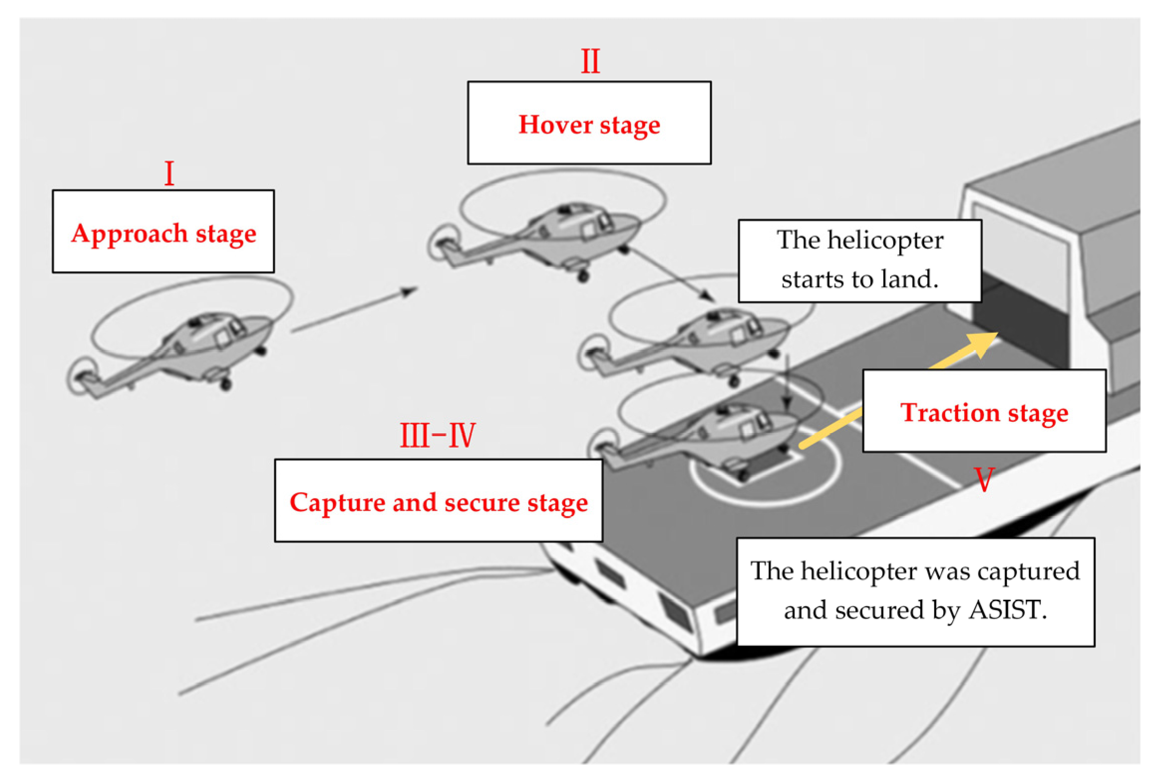
- Approach stage: The shipborne helicopter approaches the ship from a distance.
- Hover stage: The shipborne helicopter hovers above the deck.
- Capture stage: The shipborne helicopter is captured by ASIST.
- Secure stage: The shipborne helicopter is secured to the deck by ASIST.
- Traction stage: The shipborne helicopter is towed to the designated position by ASIST.
2. Working Conditions Analysis of ASIST
2.1. Introduction to Working Principle
- Approach stage
- 2.
- Hover stage
- 3.
- Capture stage
- 4.
- Secure stage
- 5.
- Traction stage
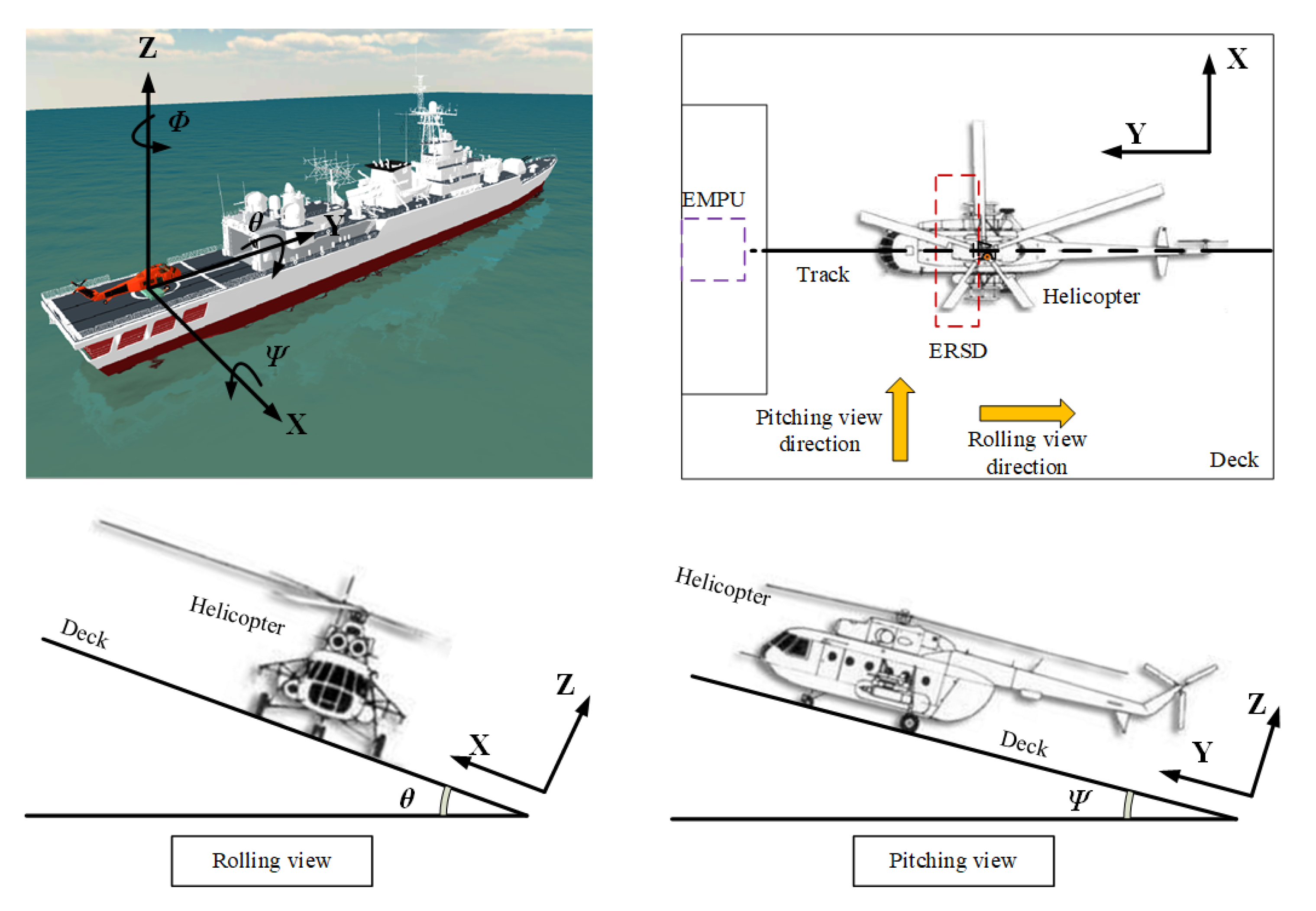
2.2. Working Conditions Analysis
- Capture stage
- 2.
- Traction stage
- In the capture stage
- In the traction stage
3. Design of the EASIST Transmission System
3.1. The Actuators
3.1.1. EMPU
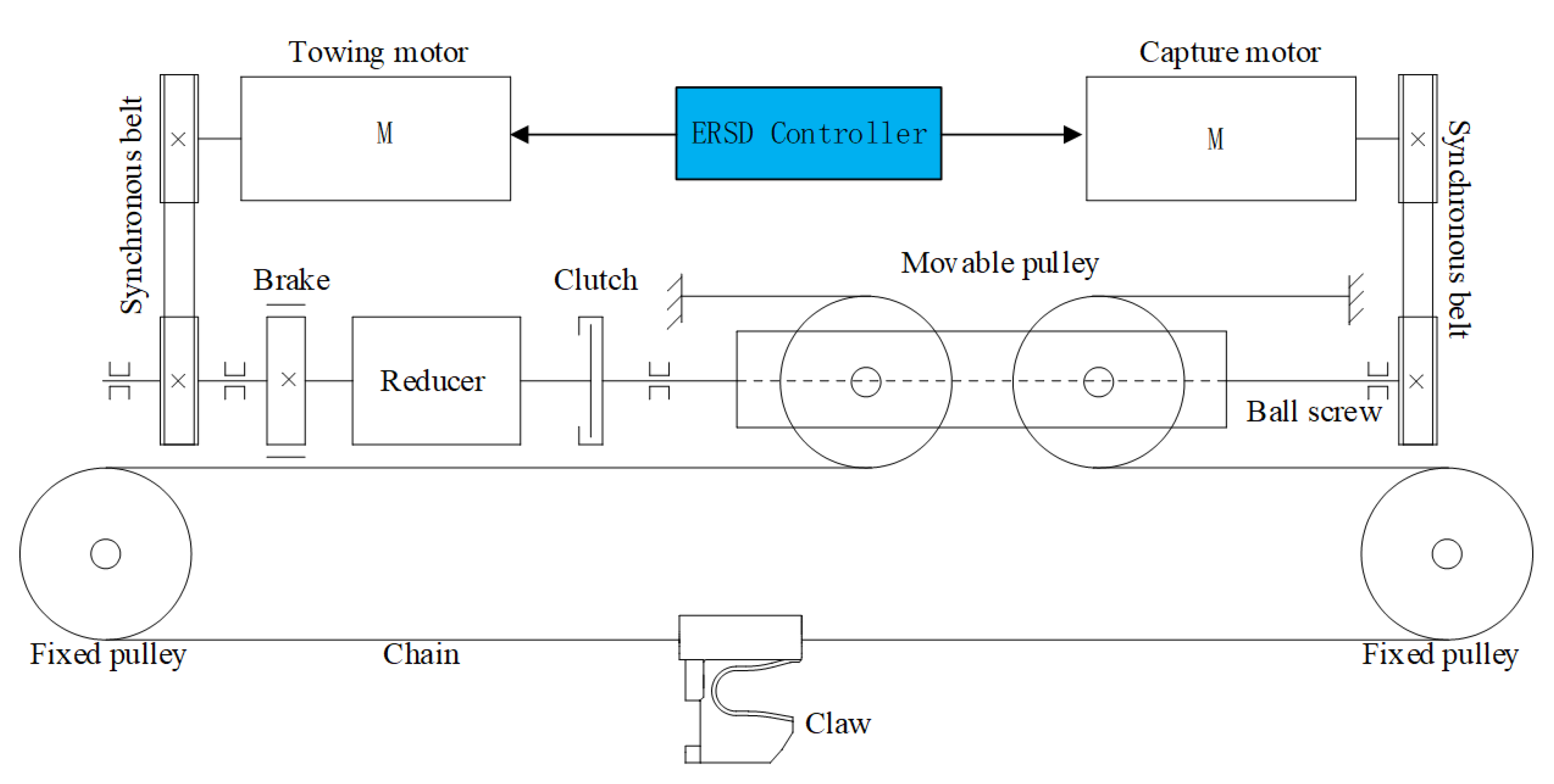
3.1.2. ERSD
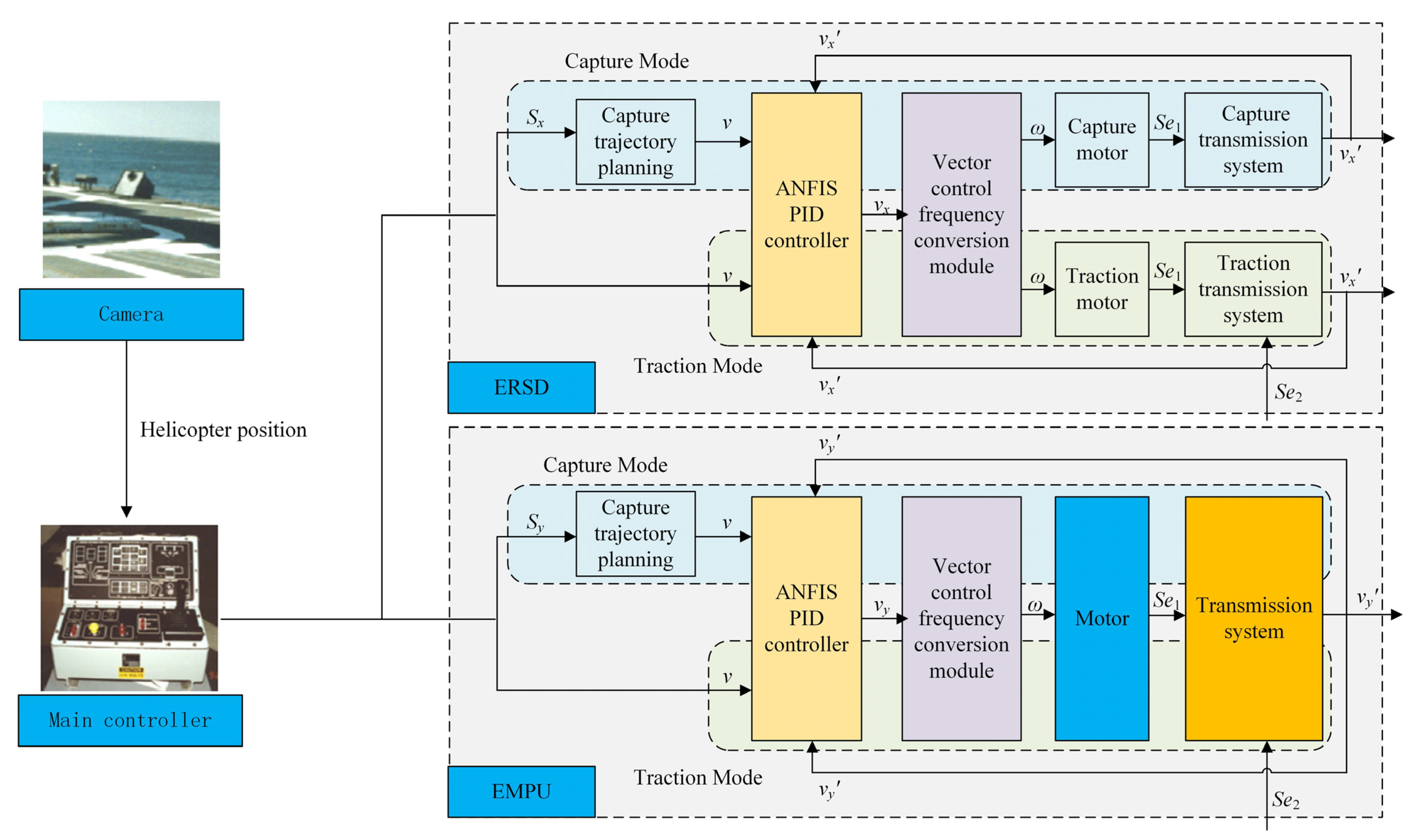
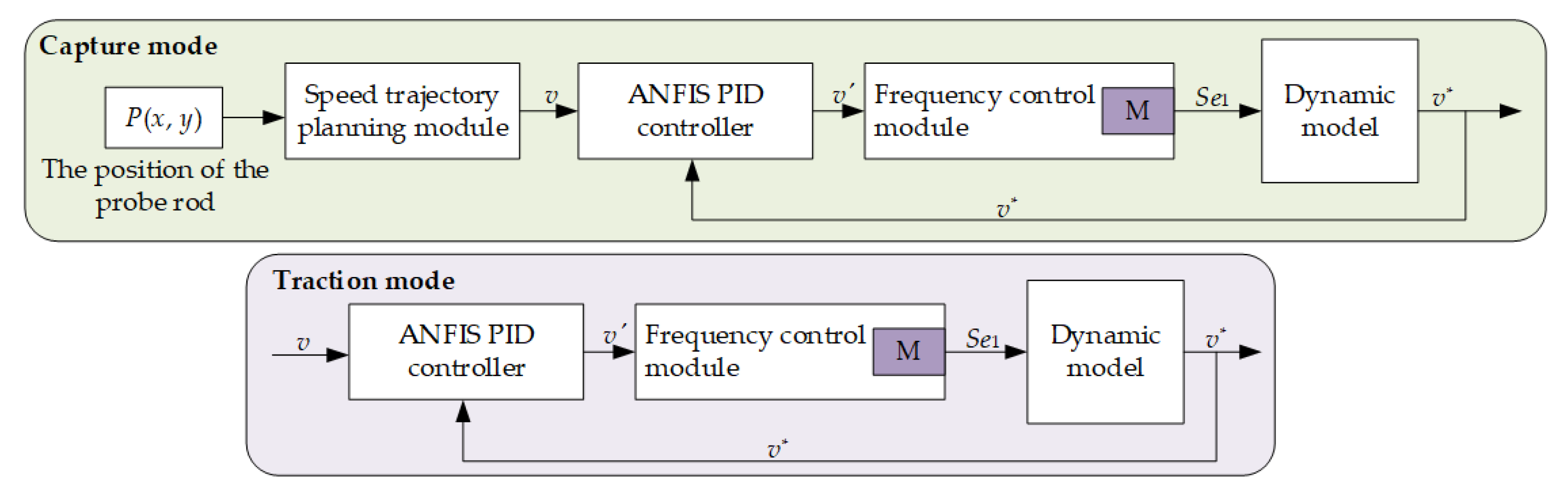
3.2. The Controller
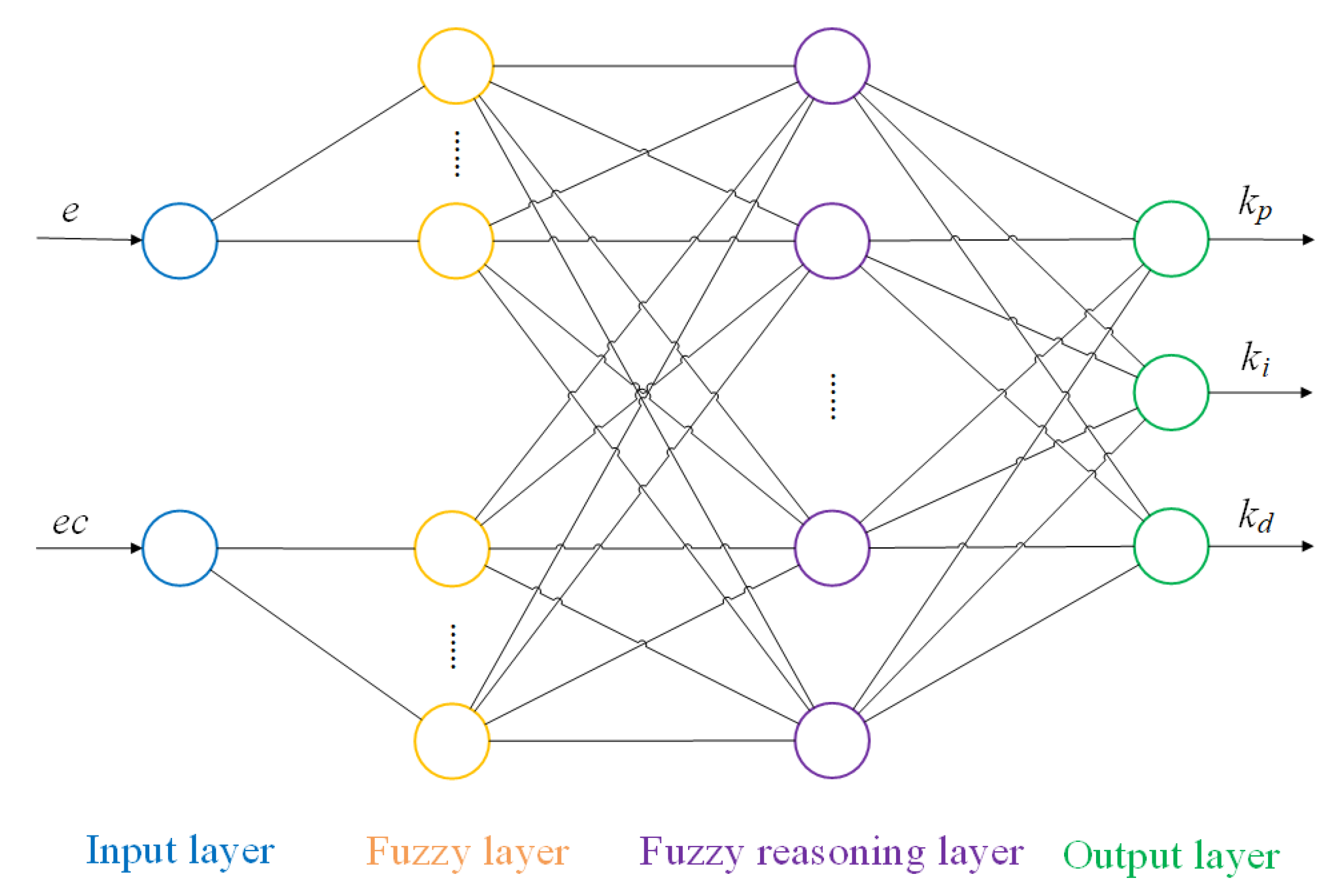
3.2.1. ANFIS PID Controller
- The first layer: the input layer.
- The second layer: the fuzzy layer.
- The third layer: the fuzzy reasoning layer.
- The fourth layer: the output layer.
- Learning algorithm.
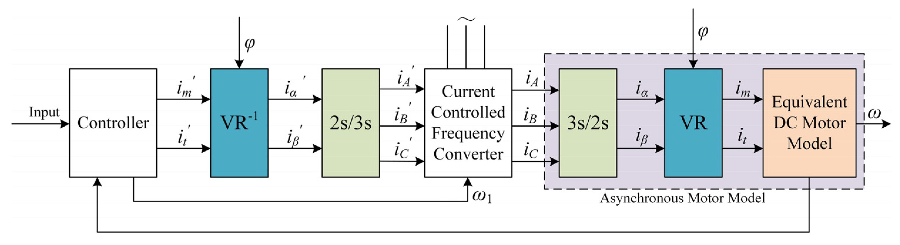
3.2.2. Vector-Controlled Converter
- -
- Ψr is rotor flux;
- -
- ism, ist are stator current;
- -
- Lr, Lm are rotor inductance and stator/rotor mutual inductance;
- -
- Rr is rotor resistance, Lr is rotor inductance, ;
- -
- p is the differential operator;
- -
- ωs is the angular velocity of the coordinate axis d-q relative to the rotor;
- -
- ω1 is the angular velocity of the coordinate axis d-q relative to the stator;
- -
- ω is the rotor angular velocity of the asynchronous motor;
- -
- np is the polar logarithm;
- -
- Te is the motor torque [42].
4. Key Characteristics Analysis
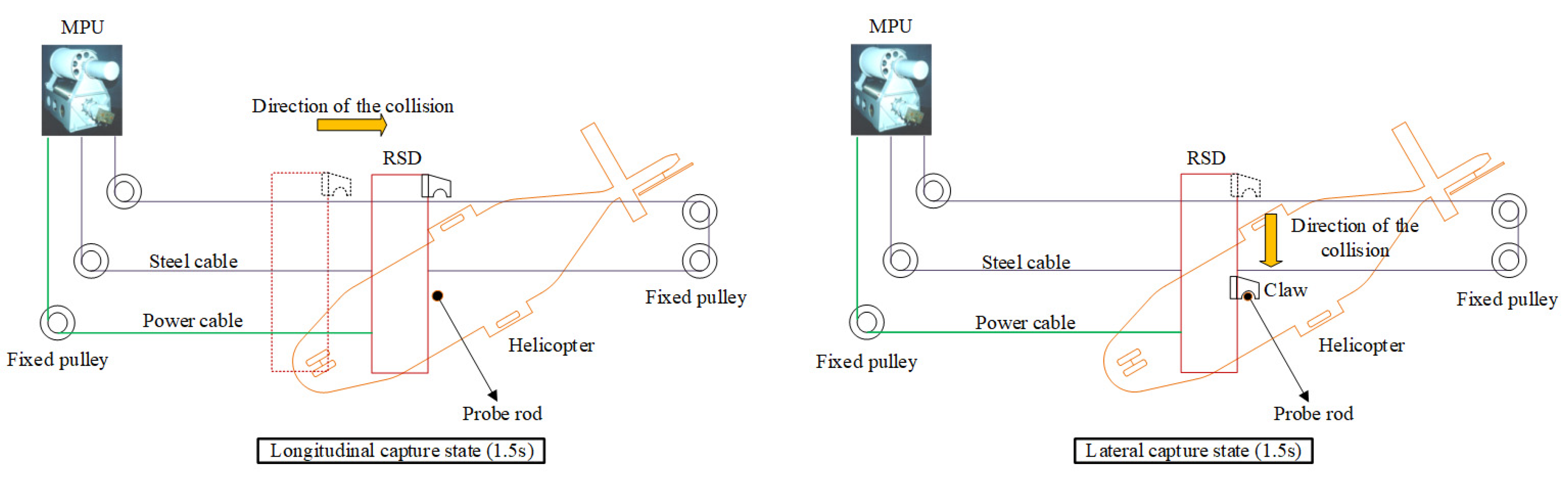
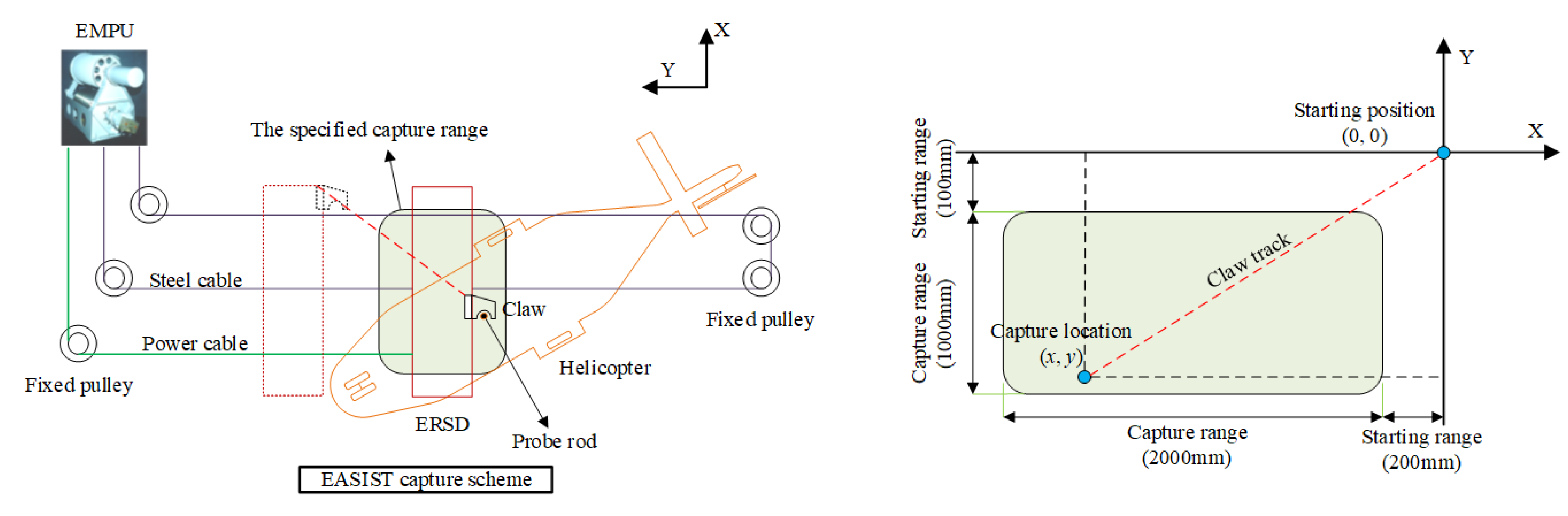
4.1. Capture Characteristic
- The claw displacement is determined.
- The claw accelerates from rest.
- The claw impacts the probe rod at a low speed.
- -
- , ;
- -
- tma is the required time of acceleration;
- -
- tmd is the required time of deceleration;
- -
- tc is the time of constant velocity.
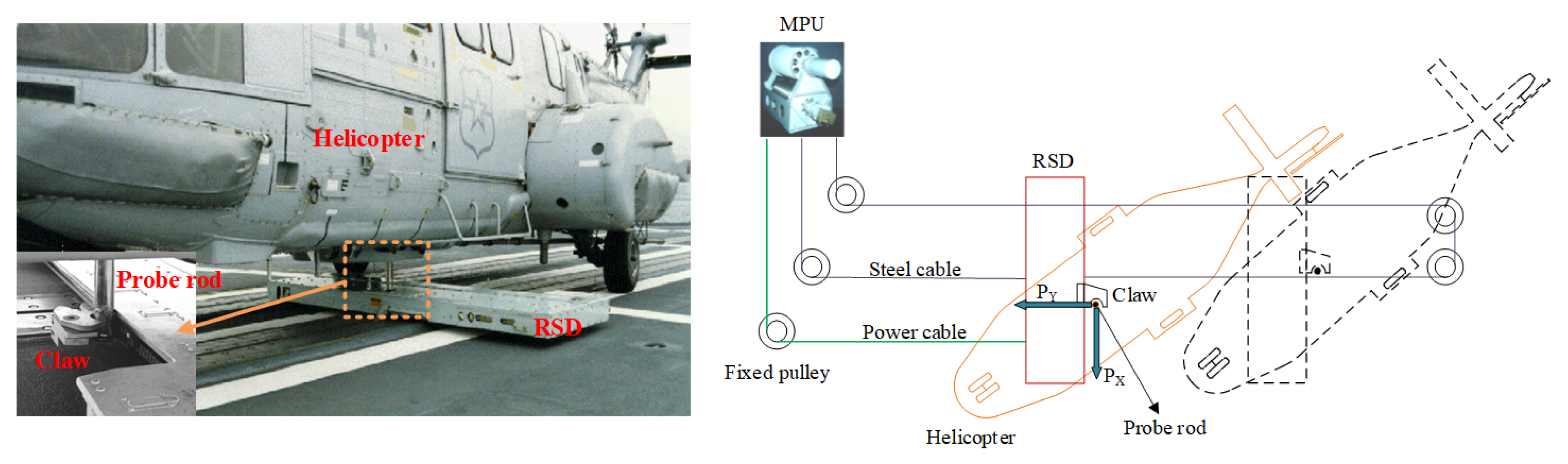
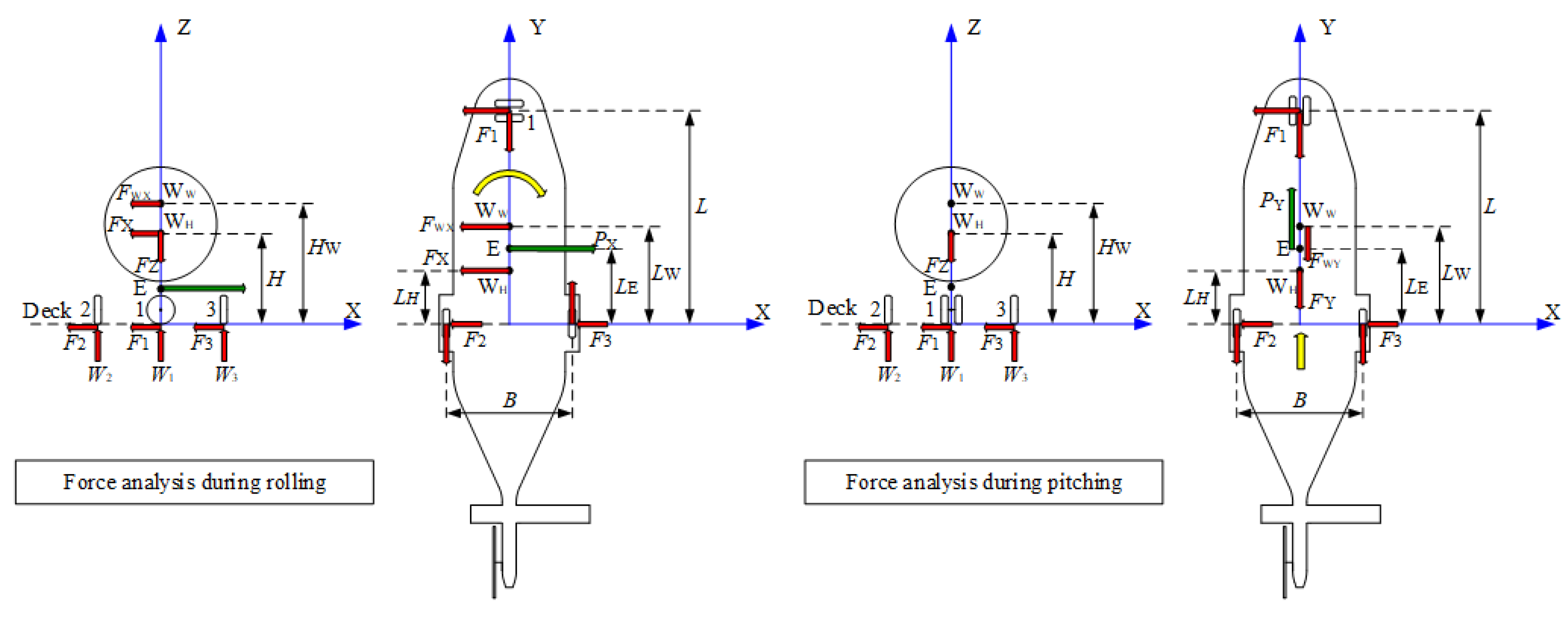
4.2. Traction Characteristic
- 1.
- In Figure 13, lateral resistance is maximum when the following three conditions are met:
- The card-axis of the front wheel is deflected by 90°;
- The wind is blowing along the negative direction of the X-axis;
- The claw pushes the helicopter in the direction of the yellow arrow.
- 2.
- In Figure 13, the longitudinal resistance is maximum when the following three conditions are met:
- The card-axis of the front wheel is deflected 0°;
- The wind is blowing along the negative direction of the Y-axis;
- The claw pushes the helicopter forward in the direction of the yellow arrow.
- Assume that the thrust force required by the claw is PY.
5. System Modeling and Simulation
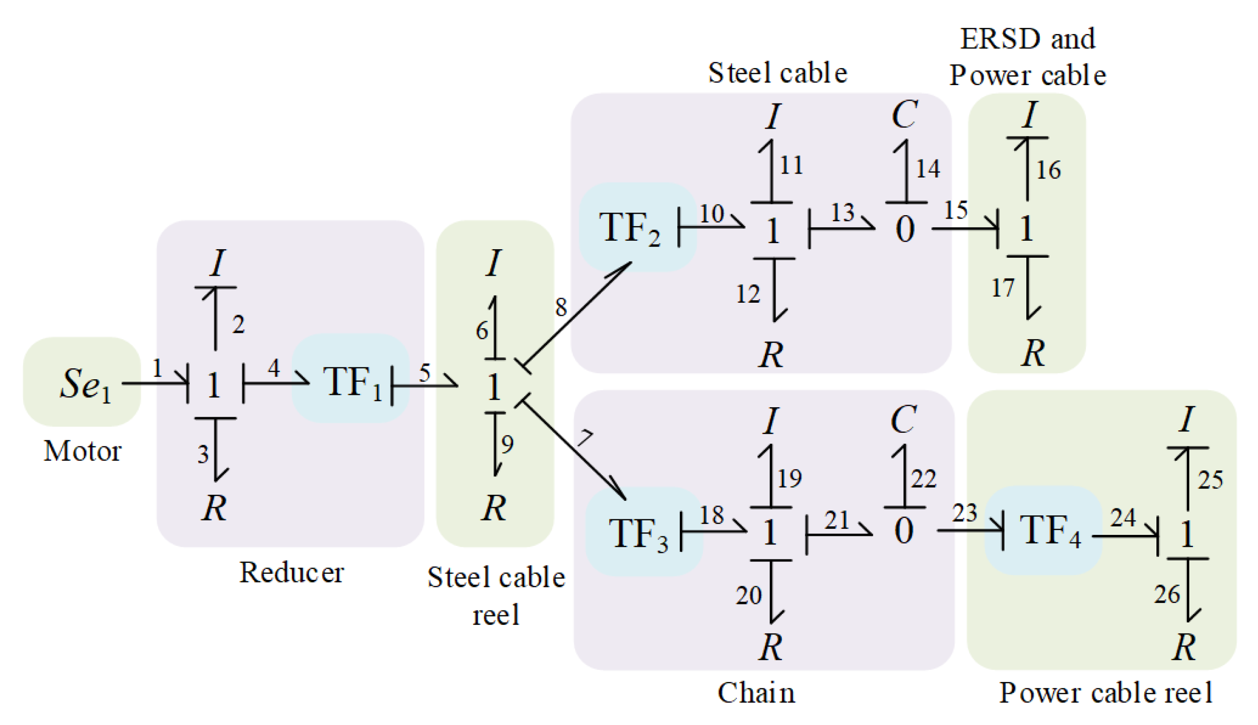
5.1. System Modeling of Capture Condition
- The driving torque of the asynchronous motor (Potential Source) drives the reducer to rotate (Inertia Element and Resistive Element).
- The reducer (Converter) drives the steel cable reel to rotate (Inertia Element and Resistive Element).
- The steel cable reel transforms rotational motion to straight motion by the steel cable (Converter) and the chain (Converter).
- The steel cable (Inertia Element and Resistive Element) drives ERSD and power cable (Inertia Element and Resistive Element) to move quickly. In contrast, the chain (Inertia Element and Resistive Element) drives the power cable reel to rotate (Converter, Inertia Element, and Resistive Element).
- The chain and steel cable length varies with the tensile force (Capacitive Element).
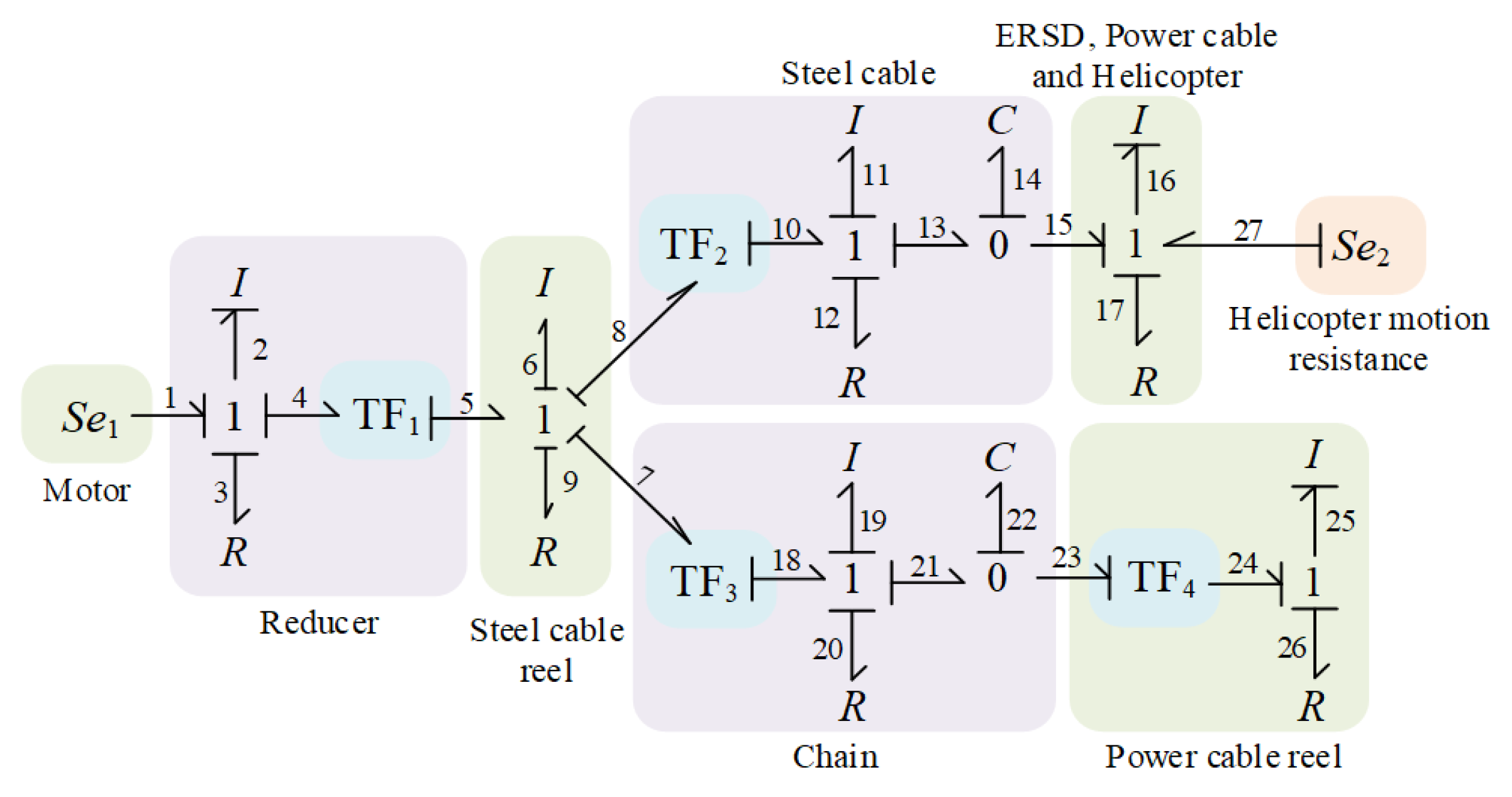
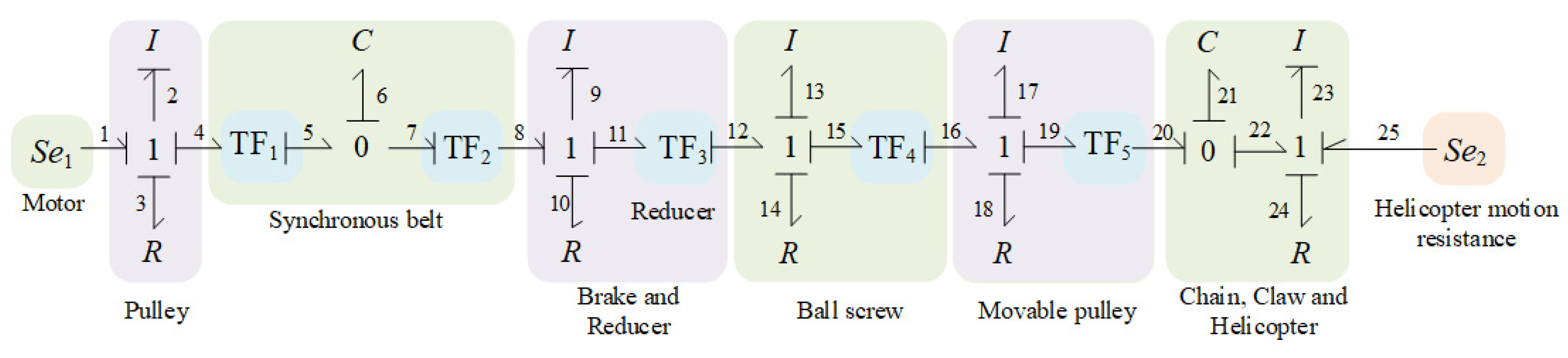
5.2. System Modeling of Traction Condition
5.3. System Simulation
- Capture simulation: This test is used to verify whether the capture time meets the requirements and whether the final capture speed can be significantly reduced.
- Traction simulation: The purpose of this test is to verify whether EASIST can adjust the moving speed of the claw in real time according to the system input when performing the traction task.
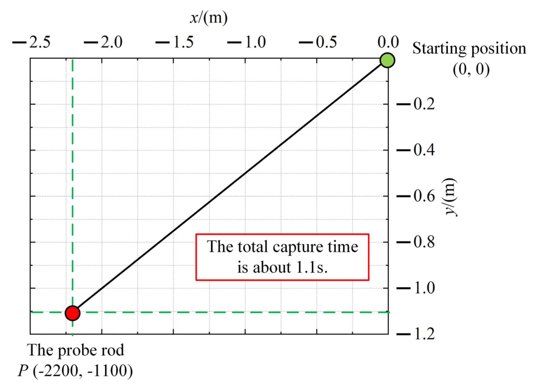
5.3.1. Capture Simulation
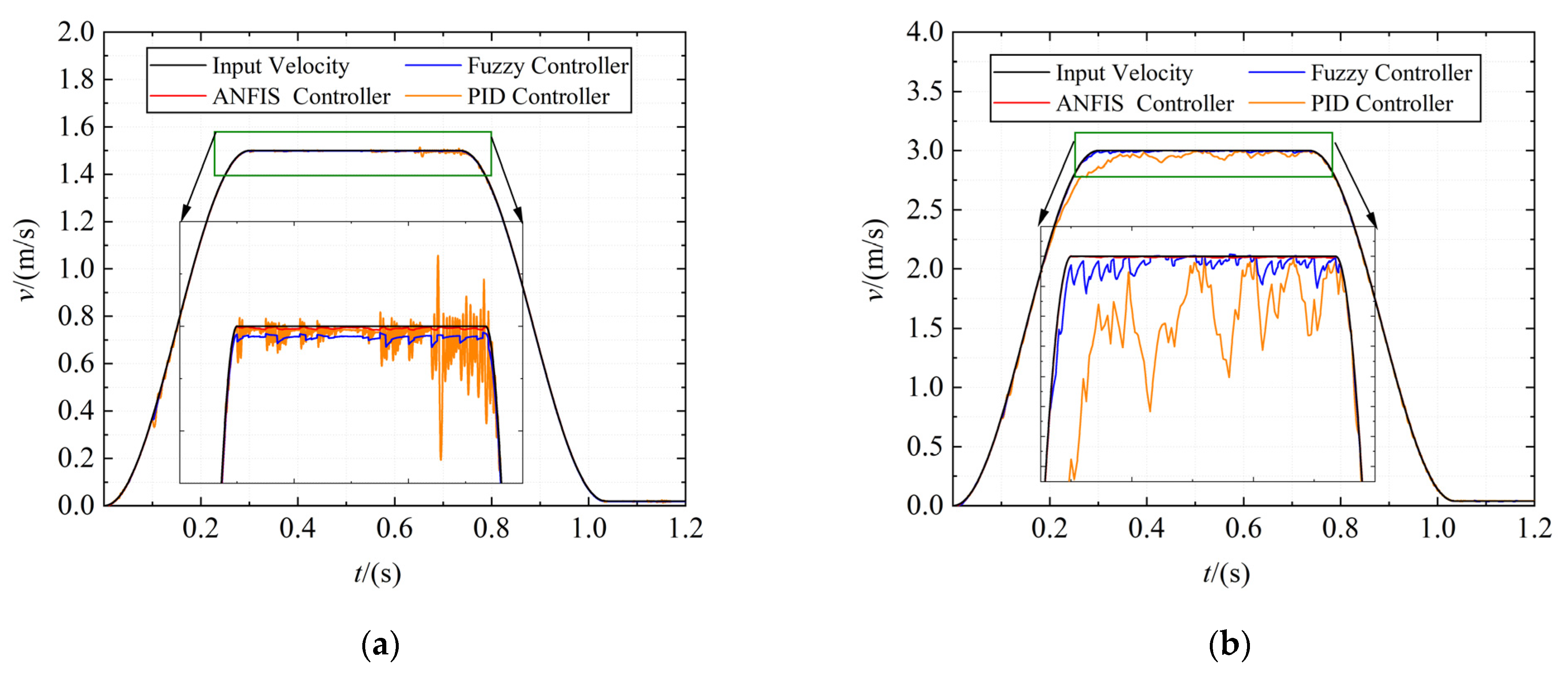
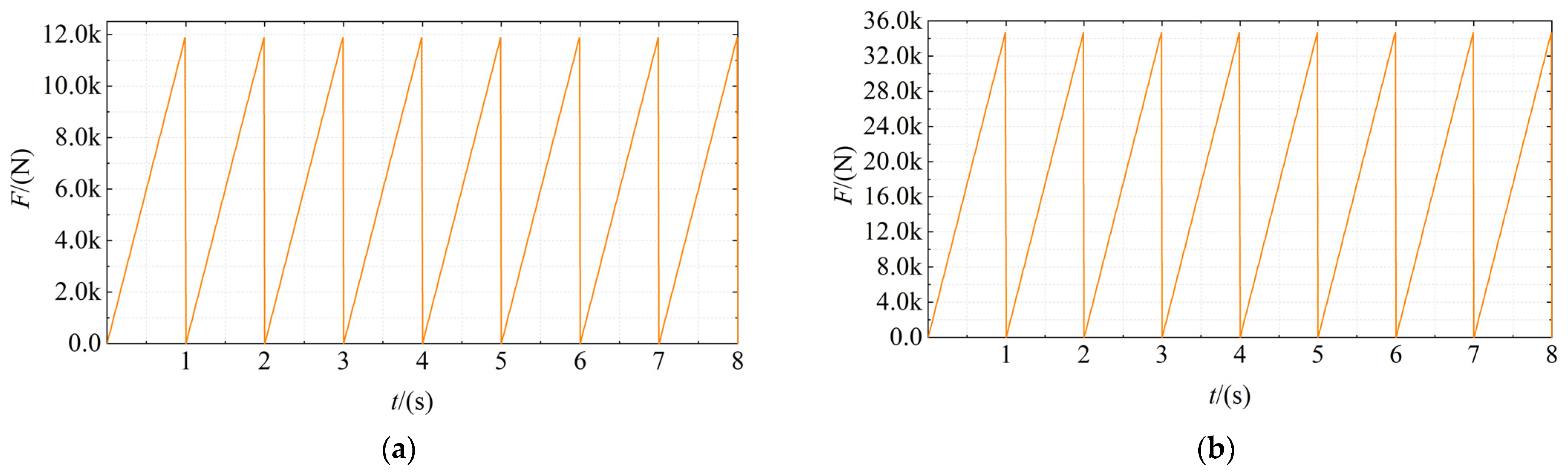
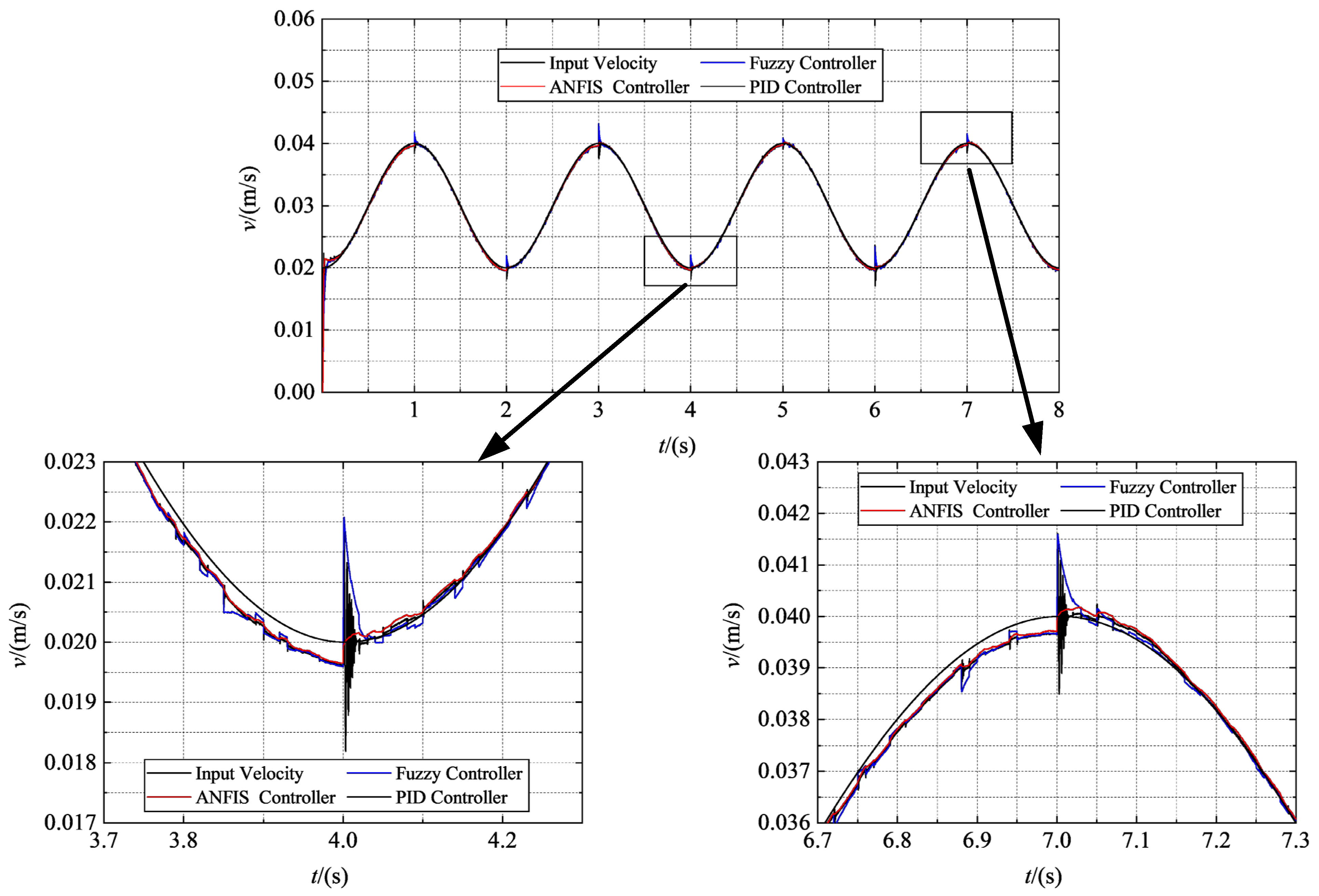
5.3.2. Traction Simulation
6. Conclusions
- A new capture scheme was designed. This scheme reduces the maximum capture time by about 60% while the original functional requirements remain unchanged. In addition, the capture speed is further limited, which can reduce the capture force significantly. This result will enable EASIST to be compatible with small shipborne aircraft.
- Compared with the fuzzy and PID controller, the designed ANFIS controller has a better speed control effect. The ANFIS controller can achieve a superior speed tracking effect under the maximum loading force during the traction task. This result is of great significance for improving the traction efficiency of EASIST.
Author Contributions
Funding
Institutional Review Board Statement
Informed Consent Statement
Conflicts of Interest
References
- Taymourtash, N.; Zagaglia, D.; Zanotti, A.; Muscarello, V.; Gibertini, G.; Quaranta, G. Experimental study of a helicopter model in shipboard operations. Aerosp. Sci. Technol. 2021, 115, 106774. [Google Scholar] [CrossRef]
- Guo, Y.; Wang, W.; Zhang, S.; Xu, W. Research on Attack Mode Selection of Helicopter Hovering and Forward for Dropping Torpedo in the Air. In Proceedings of the 2021 IEEE 6th International Conference on Computer and Communication Systems (ICCCS), Chengdu, China, 23–26 April 2021. [Google Scholar]
- Zheng, J. A Test Method for Helicopter Landing Gear Load. Int. J. Mech. Eng. Appl. 2021, 9, 19. [Google Scholar] [CrossRef]
- Su, D.; Xu, G.; Huang, S.; Shi, Y. Numerical investigation of rotor loads of a shipborne coaxial-rotor helicopter during a vertical landing based on moving overset mesh method. Eng. Appl. Comput. Fluid Mech. 2019, 13, 309–326. [Google Scholar] [CrossRef] [Green Version]
- Tušl, M.; Rainieri, G.; Fraboni, F.; De Angelis, M.; de Polo, M.; Pietrantoni, L.; Pingitore, A. Helicopter Pilots’ Tasks, Subjective Workload, and the Role of External Visual Cues During Shipboard Landing. J. Cogn. Eng. Decis. Mak. 2020, 14, 242–257. [Google Scholar] [CrossRef]
- Zhang, Z.; Liu, Q.; Zhao, D.; Wang, L.; Yang, P. Research on Shipborne Helicopter Electric Rapid Secure Device: System De-sign, Modeling, and Simulation. Sensors 2022, 22, 1514. [Google Scholar] [CrossRef]
- Lu, Y.; Chang, X.; Chuang, Z.; Xing, J.; Zhou, Z.; Zhang, X. Numerical investigation of the unsteady coupling airflow impact of a full-scale warship with a helicopter during shipboard landing. Eng. Appl. Comput. Fluid Mech. 2020, 14, 954–979. [Google Scholar] [CrossRef]
- Greer, W.B.; Sultan, C. Infinite horizon model predictive control tracking application to helicopters. Aerosp. Sci. Technol. 2020, 98, 105675. [Google Scholar] [CrossRef]
- Yu, X.; Yang, J.; Li, S. Disturbance observer-based autonomous landing control of unmanned helicopters on moving ship-board. Nonlinear Dyn. 2020, 102, 131–150. [Google Scholar] [CrossRef]
- Owen, I.; Lee, R.; Wall, A.; Fernandez, N. The NATO generic destroyer–a shared geometry for collaborative research into modelling and simulation of shipboard helicopter launch and recovery. Ocean Eng. 2021, 228, 108428. [Google Scholar] [CrossRef]
- Zhao, D.; Yang, H.; Yao, S.; Ni, T. Numerical investigation for coupled rotor/ship flowfield using two models based on the momentum source method. Eng. Appl. Comp. Fluid. 2021, 15, 1902–1918. [Google Scholar]
- Shi, Y.; Li, G.; Su, D.; Xu, G. Numerical investigation on the ship/multi-helicopter dynamic interface. Aerosp. Sci. Technol. 2020, 106, 106175. [Google Scholar] [CrossRef]
- Li, Y.; Zhang, Z.; Xiong, Z.; Xiao, J.; Li, G. Collision modeling method of ship-board helicopter landing. Syst. Eng. Electron. 2015, 430, 1691–1696. [Google Scholar]
- Zhao, D.; Yang, H.; Giuseppe, C.; Li, W.; Ni, T.; Yao, S. Modeling and analysis of landing collision dynamics for a shipborne helicopter. Front. Mech. Eng. 2021, 16, 151–162. [Google Scholar] [CrossRef]
- Zhao, D.; Wang, Q.; Zhang, Z. Extenics theory for reliability assessment of carrier helicopter based on analytic hierarchy process. J. Jilin Univ. Eng. Technol. 2016, 46, 1528–1531. [Google Scholar]
- Wang, Q.; Zhao, D.; Wei, H.; Zhao, Y. Study of the landing dynamics of carrier based helicopter under complex sea conditions. J. Northeast. Univ. Nat. Sci. 2017, 38, 1595–1600. [Google Scholar]
- Wang, Q.; Zhao, D.; Zhao, Y.; Chen, N. Dynamic analysis of carrier helicopter on complex. J. Jilin Univ. Eng. Technol. 2017, 47, 1109–1113. [Google Scholar]
- Sher, F.; Raore, D.; Klemeš, J.J.; Rafi-Ul-Shan, P.M.; Khzouz, M.; Marintseva, K.; Razmkhah, O. Unprecedented Impacts of Aviation Emissions on Global Environmental and Climate Change Scenario. Curr. Pollut. Rep. 2021, 7, 549–564. [Google Scholar] [CrossRef] [PubMed]
- Sher, F.; Hazafa, A.; Marintseva, K.; Rasheed, T.; Ali, U.; Rashid, T.; Babu, A.; Khzouz, M. Fully solar powered Doncaster Sheffield Airport: Energy evaluation, glare analysis and CO2 mitigation. Sustain. Energy Technol. Assess. 2021, 45, 101122. [Google Scholar] [CrossRef]
- Boukhalfa, G.; Belkacem, S.; Chikhi, A.; Benaggoune, S. Genetic algorithm and particle swarm optimization tuned fuzzy PID controller on direct torque control of dual star induction motor. J. Cent. South Univ. 2019, 26, 1886–1896. [Google Scholar] [CrossRef]
- Qi, X.; Su, T.; Zhou, K.; Yang, J.C.; Gan, X.P.; Zhang, Y.C. Development of AC Motor Model Predictive Control Strategy: An Overview. Proc. CSEE 2021, 677, 6408–6419. [Google Scholar]
- Sartorius, A.R.; de Jesus Moreno, J.; Pinon, O.; Ruiz, A.E. A new approach for adjusting scale factor in fuzzy PD+ I controllers with anti-windup. J. Intell. Fuzzy Syst. 2014, 27, 2319–2326. [Google Scholar] [CrossRef]
- Arpaci, H.; Ozguven, O.F. Design of Adaptive Fractional-Order PID Controller to Enhance Robustness by Means of Adaptive Network Fuzzy Inference System. Int. J. Fuzzy Syst. 2017, 19, 1118–1131. [Google Scholar] [CrossRef]
- Milovanović, M.B.; Antić, D.S.; Milojković, M.T.; Nikolić, S.S.; Perić, S.L.; Spasić, M.D. Adaptive PID control based on orthogonal endocrine neural networks. Neural Netw. 2016, 84, 80–90. [Google Scholar] [CrossRef] [PubMed]
- Premkumar, K.; Manikandan, B. Adaptive Neuro-Fuzzy Inference System based speed controller for brushless DC motor. Neurocomputing 2014, 138, 260–270. [Google Scholar] [CrossRef]
- Premkumar, K.; Manikandan, B. Fuzzy PID supervised online ANFIS based speed controller for brushless dc motor. Neurocomputing 2015, 157, 76–90. [Google Scholar] [CrossRef]
- Navaneethakkannan, C.; Sudha, M. Analysis and Implementation of ANFIS-based Rotor Position Controller for BLDC Motors. J. Power Electron. 2016, 16, 564–571. [Google Scholar] [CrossRef] [Green Version]
- Eski, I.; Yıldırım, Ş. Neural network-based fuzzy inference system for speed control of heavy duty vehicles with electronic throttle control system. Neural Comput. Appl. 2017, 28, 907–916. [Google Scholar] [CrossRef]
- Wang, Y.; Zhao, D.; Wang, L.; Zhang, Z.; Wang, L.; Hu, Y. Dynamic simulation and analysis of the elevating mechanism of a forklift based on a power bond graph. J. Mech. Sci. Technol. 2016, 30, 4043–4048. [Google Scholar] [CrossRef]
- Rodríguez-Guillén, J.; Salas-Cabrera, R.; García-Vite, P.M. Bond Graph as a formal methodology for obtaining a wind turbine drive train model in the per-unit system. Int. J. Electr. Power Energy Syst. 2021, 124, 106382. [Google Scholar] [CrossRef]
- Karimian, S.; Jahanbin, Z. Bond graph modeling of a typical flapping wing micro-air-vehicle with the elastic articulated wings. Meccanica 2020, 55, 1263–1294. [Google Scholar] [CrossRef]
- Badoud, A.E.; Merahi, F.; Bouamama, B.O.; Mekhilef, S. Bond graph modeling, design and experimental validation of a photovoltaic/fuel cell/ electrolyzer/battery hybrid power system. Int. J. Hydrogen Energy 2021, 46, 24011–24027. [Google Scholar] [CrossRef]
- Song, K.; Wang, Y.; An, C.; Xu, H.; Ding, Y. Design and Validation of Energy Management Strategy for Extended-Range Fuel Cell Electric Vehicle Using Bond Graph Method. Energies 2021, 14, 380. [Google Scholar] [CrossRef]
- Yahi, F.; Belhamel, M.; Bouzeffour, F.; Sari, O. Structured dynamic modeling and simulation of parabolic trough solar collector using bond graph approach. Sol. Energy 2020, 196, 27–38. [Google Scholar] [CrossRef]
- Liu, W.; Li, L.; Cai, W.; Li, C.; Li, L.; Chen, X.; Sutherland, J.W. Dynamic characteristics and energy consumption modelling of machine tools based on bond graph theory. Energy 2020, 212, 118767. [Google Scholar] [CrossRef]
- Mezghani, D.; Mami, A.; Dauphin-Tanguy, G. Bond graph modelling and control enhancement of an off-grid hybrid pumping system by frequency optimization. Int. J. Numer. Model. Electron. Netw. Devices Fields 2020, 33, e2717. [Google Scholar] [CrossRef]
- Ghimire, P.; Zadeh, M.; Pedersen, E.; Thorstensen, J. Dynamic Modeling, Simulation, and Testing of a Marine DC Hybrid Power System. IEEE Trans. Transp. Electrif. 2021, 7, 905–919. [Google Scholar] [CrossRef]
- Aftabi Talami, M.; Jamali, A.; Nariman-zadeh, N. A new method for extracting the state equations from bond graph of dynamical systems (SEBG method). Int. J. Gen. Syst. 2021, 50, 703–723. [Google Scholar] [CrossRef]
- Schock, A.R. Development of a Planar Shipboard Skid-Equipped Rotary-Wing Aircraft Manoeuvring and Securing Simulation. Ph.D. Thesis, Carleton University, Ottawa, ON, Canada, 2020. [Google Scholar]
- Li, B.; Wang, L.; Zhang, S.; Wang, J. Research on Loop Decoupling Control Based on Fuzzy RBF Neural Network. In Proceedings of the 2021 33rd Chinese Control and Decision Conference (CCDC), Kunming, China, 22–24 May 2021. [Google Scholar]
- Sher, F.; Chen, S.; Raza, A.; Rasheed, T.; Razmkhah, O.; Rashid, T.; Rafi-Ul-Shan, P.M.; Erten, B. Novel strategies to reduce engine emissions and improve energy efficiency in hybrid vehicles. Clean. Eng. Technol. 2021, 2, 100074. [Google Scholar] [CrossRef]
- Liu, Q.; Zhang, Z.; Zhao, D.; Wang, L.; Meng, F.; Liu, C. Research on Speed Tracking of Asynchronous Motor Based on Fuzzy Control and Vector Control. In Proceedings of the 2020 39th Chinese Control Conference (CCC), Shenyang, China, 27–29 July 2020. [Google Scholar]
- Kan, C.; Bao, X.; Wang, X.; Xiong, F.; Ma, B. Overview and Recent developments of Brushless Doubly-fed Machines. Proc. CSEE 2018, 38, 3939–3959. [Google Scholar]
- Wang, L.; Lin, L.; Chang, Y.; Xue, F. Velocity Planning Algorithm in One-Dimensional Linear Motion for Astronaut Virtual Training. J. Astronaut. 2021, 42, 1600–1609. [Google Scholar]
- Li, Z.; Wang, T.; Wang, B.; Guo, Z.; Chen, D. Trajectory planning for manipulator in Cartesian space based on constrained S-curve velocity. CAAI T. Intell. Sys. 2019, 14, 655–661. [Google Scholar]
- Hussain, S.Z.; Kausar, Z.; Koreshi, Z.U.; Sheikh, S.R.; Rehman, H.Z.U.; Yaqoob, H.; Shah, M.F.; Abdullah, A.; Sher, F. Feed-back Control of Melt Pool Area in Selective Laser Melting Additive Manufacturing Process. Processes 2021, 9, 1547. [Google Scholar] [CrossRef]
- Rashid, T.; Taqvi, S.A.A.; Sher, F.; Rubab, S.; Thanabalan, M.; Bilal, M.; Islam, B.U. Enhanced lignin extraction and optimisation from oil palm biomass using neural network modelling. Fuel 2021, 293, 120485. [Google Scholar] [CrossRef]


| Parameters | Symbol | Value | Parameters | Symbol | Value |
|---|---|---|---|---|---|
| Distance between the mass center and the Z-axis | LH | 0.9 m | Helicopter mass | MH | 10,000 kg |
| Distance between the force point and the Z-axis | LE | 0.9 m | Distance between the front wheel and rear wheel centerline | L | 7 m |
| Distance between the two rear wheels | B | 3.5 m | Height from the mass center to the deck | H | 2 m |
| Distance from the wind center to the Z-axis | LW | 0.9 m | Height from the wind center to the deck | HW | 1.3 m |
| Lateral wind action constant | AXCW | 20 | Longitudinal wind force action constant | AYCW | 2.5 |
| Air density | ρ | 1.29 kg/m3 | Rolling friction coefficient | f | 0.02 |
| Maximum roll angle | θ | 10° | Maximum pitch angle | λ | 2.5° |
| Maximum lateral acceleration | ax | 1 m/s2 | Maximum longitudinal acceleration | ay | 1 m/s2 |
| Maximum vertical acceleration | az | 0.5 m/s2 | Maximum wind speed | vW | 12 m/s |
| Parts | Physical Meaning | Character | Value | Units |
|---|---|---|---|---|
| Asynchronous motor | Driving torque | Potential Source | -- | -- |
| Reducer | The moment of inertia | Inertia Element | 5.7 × 10⁻³ | kg·m2 |
| Rotational damping | Resistive Element | 11.4 × 10⁻⁴ | N·m·s/rad | |
| Reduction ratio | Converter | 50 | -- | |
| Steel cable reel | The moment of inertia | Inertia Element | 1.721 | kg·m2 |
| Rotational damping | Resistive Element | 7.9 × 10⁻³ | N·m·s/rad | |
| Steel cable | Rotational motion to Straight motion | Converter | 1/0.3 | rad/m |
| Mass | Inertia Element | 57 | kg | |
| Movement damping | Resistive Element | 18.12 | N·s/m | |
| Elastic coefficient | Capacitive Element | 0.3 × 10⁻¹⁰ | m/N | |
| ERSD and Power cable | Mass | Inertia Element | 1500 | kg |
| Movement damping | Resistive Element | 88.1 | N·s/m | |
| Chain | Rotational motion to Straight motion | Converter | 1/(72 × 10−3) | rad/m |
| Mass | Inertia Element | 3.7 | kg | |
| Movement damping | Resistive Element | 11.7 | N·s/m | |
| Elastic coefficient | Capacitive Element | 0.5 × 10⁻⁷ | m/N | |
| Power cable reel | Straight motion to rotational motion | Converter | 72 × 10−3 | m/rad |
| The moment of inertia | Inertia Element | 21 | kg | |
| Rotational damping | Resistive Element | 7.4 | N·s/m | |
| Helicopter | Motion resistance | Potential Source | -- | -- |
| Mass | Inertia Element | 104 | kg |
| Parts | Physical Meaning | Character | Value | Units |
|---|---|---|---|---|
| Asynchronous motor | Driving torque | Potential Source | -- | -- |
| Pully | The moment of inertia | Inertia Element | 1.04 × 10⁻³ | kg·m2 |
| Rotational damping | Resistive Element | 8.2 × 10⁻⁴ | N·m·s/rad | |
| Synchronous belt | Rotational motion to straight motion | Converter | 1/48.51 × 10−3 | rad/m |
| Elastic coefficient | Capacitive Element | 1/15,200 | m/N | |
| Straight motion to rotational motion | Converter | 48.51 × 10⁻³ | m/rad | |
| Brake and Reducer | The moment of inertia | Inertia Element | 3.865 × 10⁻³ | kg·m2 |
| Rotational damping | Resistive Element | 3.8 × 10⁻³ | N·m·s/rad | |
| The reduction ratio of reducer | Converter | 40 | -- | |
| Ball screw | The moment of inertia | Inertia Element | 2.295 × 10⁻² | kg·m2 |
| Rotational damping | Resistive Element | 2.5 × 10⁻³ | N·m·s/rad | |
| Rotational motion to straight motion | Converter | 2π/(20 × 10−3) | rad/m | |
| Movable pulley | Mass | Inertia Element | 35.753 | kg |
| Movement damping | Resistive Element | 40 | N·s/m | |
| Chain transmission ratio | Converter | 1/2 | -- | |
| Chain and Claw | The elastic coefficient of chain | Capacitive Element | 0.5 × 10⁻⁷ | m/N |
| Mass | Inertia Element | 44.328 | kg | |
| Movement damping | Resistive Element | 130 | N·s/m | |
| Helicopter | Motion resistance | Potential Source | -- | -- |
| Mass | Inertia Element | 104 | kg |
Publisher’s Note: MDPI stays neutral with regard to jurisdictional claims in published maps and institutional affiliations. |
© 2022 by the authors. Licensee MDPI, Basel, Switzerland. This article is an open access article distributed under the terms and conditions of the Creative Commons Attribution (CC BY) license (https://creativecommons.org/licenses/by/4.0/).
Share and Cite
Zhang, Z.; Liu, Q.; Zhao, D.; Wang, L.; Jia, T. Electrical Aircraft Ship Integrated Secure and Traverse System Design and Key Characteristics Analysis. Appl. Sci. 2022, 12, 2603. https://doi.org/10.3390/app12052603
Zhang Z, Liu Q, Zhao D, Wang L, Jia T. Electrical Aircraft Ship Integrated Secure and Traverse System Design and Key Characteristics Analysis. Applied Sciences. 2022; 12(5):2603. https://doi.org/10.3390/app12052603
Chicago/Turabian StyleZhang, Zhuxin, Qian Liu, Dingxuan Zhao, Lixin Wang, and Tuo Jia. 2022. "Electrical Aircraft Ship Integrated Secure and Traverse System Design and Key Characteristics Analysis" Applied Sciences 12, no. 5: 2603. https://doi.org/10.3390/app12052603