Article

1 to 1000 Policy: Controlling Phosphorous Pollution from Tea Farms with Bioretention Cells

1
Department of Civil Engineering, National Taipei University of Technology, Taipei 106344, Taiwan
2
Department of Civil and Construction Engineering, National Taiwan University of Science and Technology, Taipei 106335, Taiwan
3
Taipei Water Management Office, Water Resources Agency, New Taipei City 106242, Taiwan
*
Author to whom correspondence should be addressed.
Appl. Sci. 2022, 12(5), 2661; https://doi.org/10.3390/app12052661
Submission received: 26 January 2022 / Revised: 25 February 2022 / Accepted: 2 March 2022 / Published: 4 March 2022

Abstract

:
When implementing nonpoint source pollution control plans, the size or number of required controlling facilities is a very practical issue. However, quantifying nonpoint source pollution is difficult because it is generated by variable and random rainfall events. This study develops a two-stage optimization process to demonstrate the determination of the optimal bioretention cell size for tea farm pollution control. The optimization process was based on a verified watershed-scale model and a verified site-scale model. The verified watershed model was used to obtain total phosphorous (TP) reduction loads. Once the goal of watershed management was decided, the reduction loads were then allocated and the unit reduction loads were determined. Using the unit reduction loads, the verified tea farm model was used to assess the optimal bioretention cell size for tea farms. A case study using the Jinggualiao stream in the Feitsui Reservoir watershed, Taipei, Taiwan was presented. The results showed that the unit tea farm TP reduction loads were 270 g/ha-year and 326 g/ha-year to reach two water quality goals, and a total of 350 m2 and 600 m2 of bioretention cells were needed, respectively. A 1 to 1000 ratio of the standard bioretention cell area to the tea farm area is recommended as a general control rule.

1. Introduction

Water quality protection is always an important issue, and its implementation relies on comprehensive watershed management work. However, directly connecting watershed management control measures and their contributions to water quality improvement is a challenge, especially control measures on nonpoint source pollution [1,2,3,4]. Unlike continuous emissions from point sources, the impact from nonpoint source pollution is highly variable and randomly occurs in wet weather [5,6]. Therefore, the control of nonpoint source pollution is usually difficult, and any associated assessment contains high uncertainty [7,8,9]. This will impede the control of nonpoint source pollution and subsequently weaken the implementation of watershed management policy.
Many studies have proven that structural Best Management Practices (BMPs), such as constructed wetlands [10,11,12], bioretention systems [13,14,15], grass belts and swales [16] are effective. These structural BMPs are successful in removing different pollutants from surface runoff; however, how these BMPs contribute to the water quality in receiving waterbodies remains to be demonstrated. The connection between dispersed BMP measures and the resulting water quality is needed. Lintern et al. (2020) indicated that water quality did not substantially improve after massive BMP efforts, possibly because of the lack of information from field monitoring [17]. The core mission of water quality protection should start with the carry capacity of a receiving waterbody as the foundation of watershed management. The carry capacity of the environment refers to the natural ability to self-purify pollution without damaging its natural function. Some studies have used watershed model tools to link the relationship between pollution sources, including point and nonpoint sources in watersheds, and water quality [18,19,20,21]. The Total Maximum Daily Loads (TMDL) policy in the U.S. is also based on the carry capacity of a receiving waterbody and allocates the loads to different pollution sources [22]. While the carry capacity is determined as a top-down policy, another gap is found in the design of onsite control facilities. Without a quantitative goal for each site, building effective onsite BMPs is difficult.
Thus, the question is, how can a watershed-scale goal be implemented into a site-scale design? This is a very practical question. When a structural BMP aims to reduce nonpoint source pollution, the level of treatment required to match the watershed management goal must be decided. This is referred to as the optimal design for BMPs in this study. The optimal design is based on the requirement of the watershed, not the site itself. Therefore, a top-down linkage is important, and all of the control measures are designed according to the water quality goal. A process for determining an optimal onsite BMP facility is demonstrated in this study. Data from the watershed, receiving waterbody and pollution sources as well as policy-making considerations are logically integrated in this process. The process demonstrated in this study can be applied to different water quality goals, pollution sources or control measures.
The Jinggualiao stream is one of the inflow streams of the Feitsui Reservoir, Taipei, Taiwan, and it was used as a case study. The reservoir is the main water supply for Taipei and New Taipei city. To maintain the water quality of the reservoir, the inflow stream quality was considered. To avoid possible eutrophication and algae blooming, the excess nutrients in these inflow streams need to be controlled. In this reservoir watershed, nonpoint source pollution dominates the water quality because the point sources are mostly collected and treated in domestic sewage treatment plants. According to previous investigations, tea farms are regarded as the main nonpoint source pollution generators, and phosphorous (P) is the target pollutant [23,24]. The government implemented a distributed policy rather than a concentrated treatment policy to control nonpoint source pollution and built small-scale onsite treatment facilities at each tea farm. Bioretention cells were chosen within this watershed as onsite treatment BMPs. While the target pollutant (TP), pollution sources (tea farms) and control measures (bioretention cells) were already determined by the government, the number of required bioretention cells and a suitable cell size for each tea farm are not known. To solve these problems, a process was established and applied to this watershed and a tea farm case study to obtain valuable quantitative information.
Concerning the following sections: The case study and modeling tools used in this study are addressed in the Materials and Methods section. The key optimization process to determine the optimal size of the bioretention cell is also explained in this section. The Results and Discussion section first demonstrates the results of the modeling tools and their calibration and verification. After verifying the models, the results of the developed optimization process applied to the case study are addressed step by step. An overall discussion about the effectiveness of bioretention cells on water quality improvement is also included. Finally, the important remarks and findings are concluded in the last section.

2. Materials and Methods
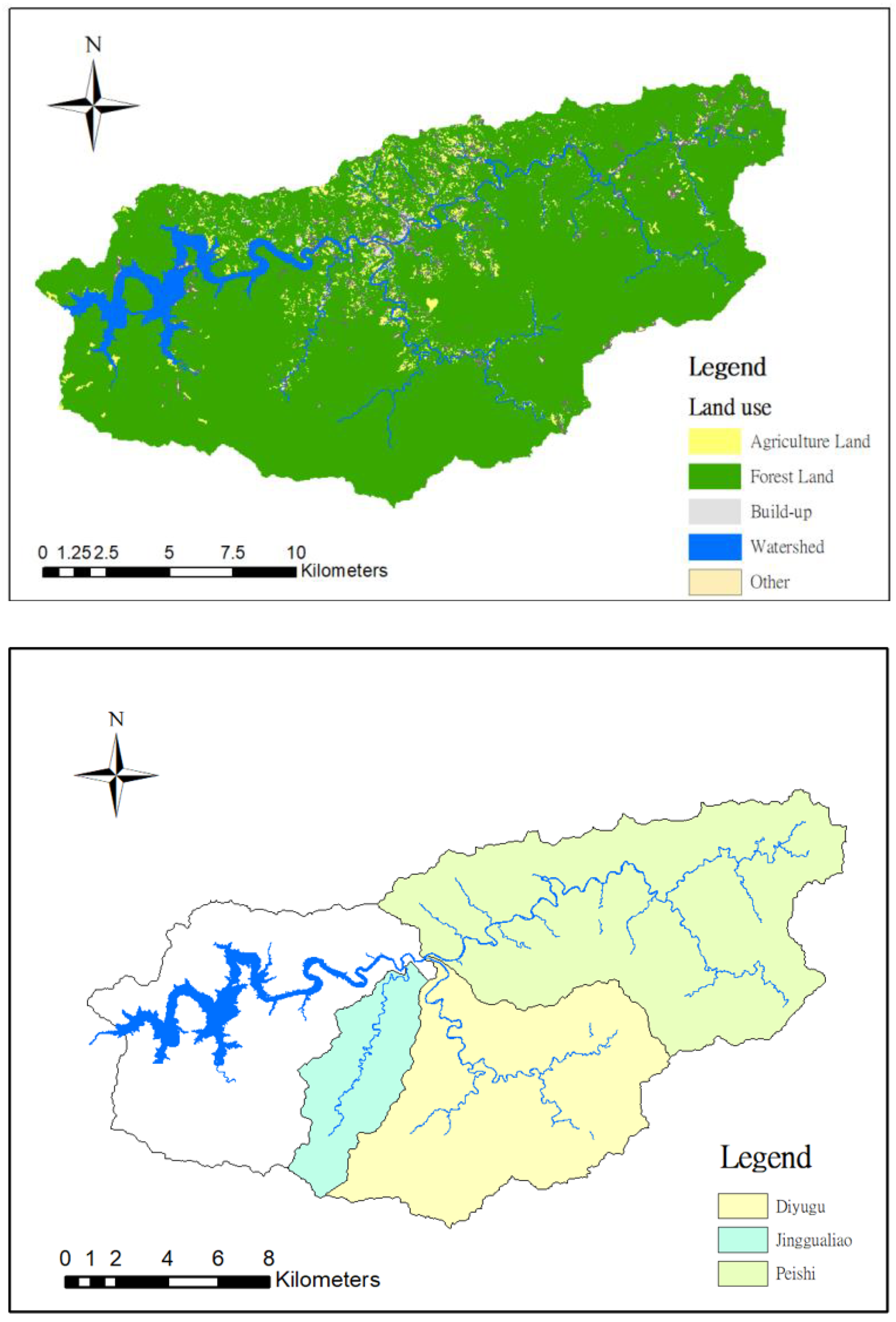
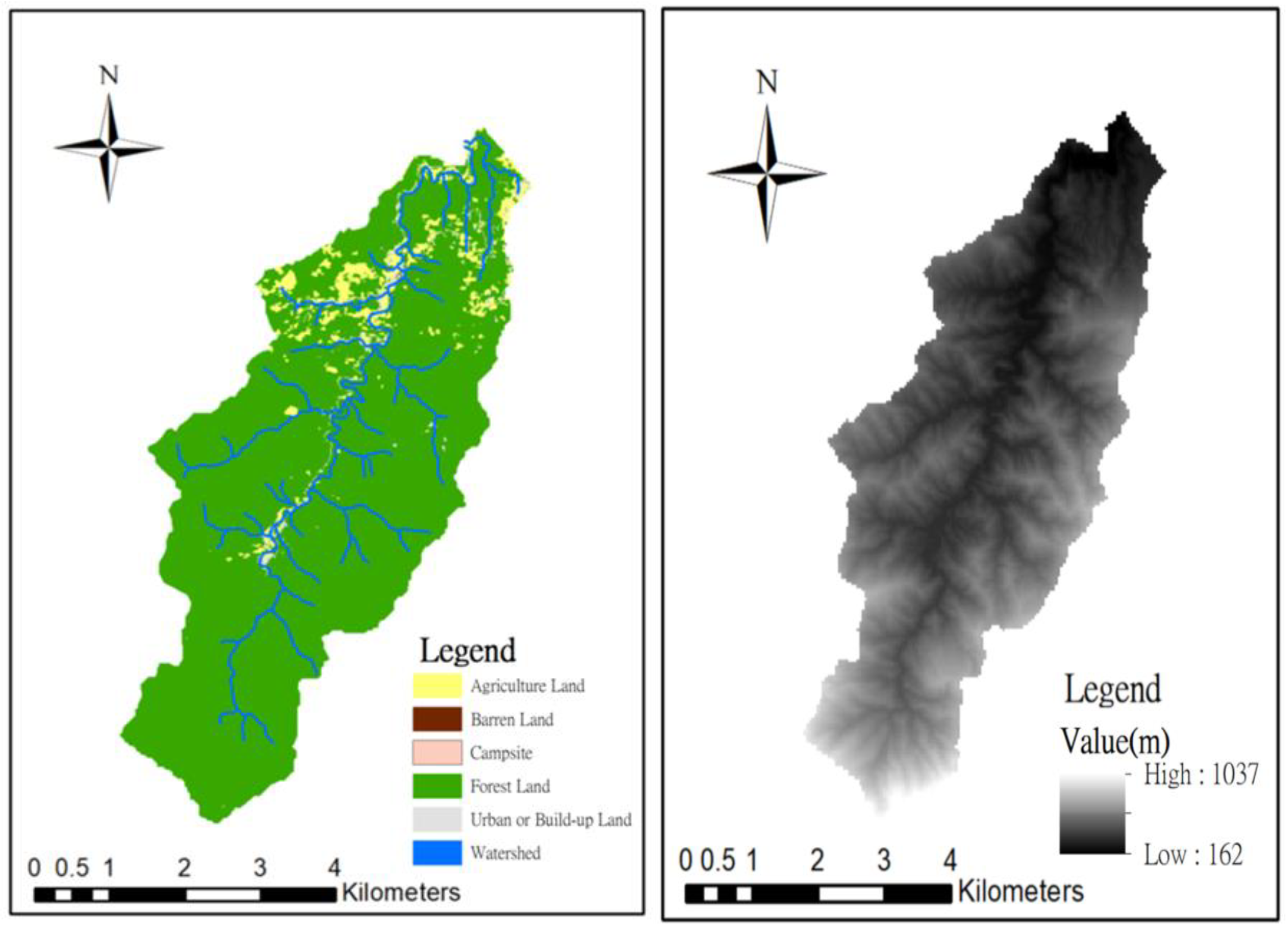
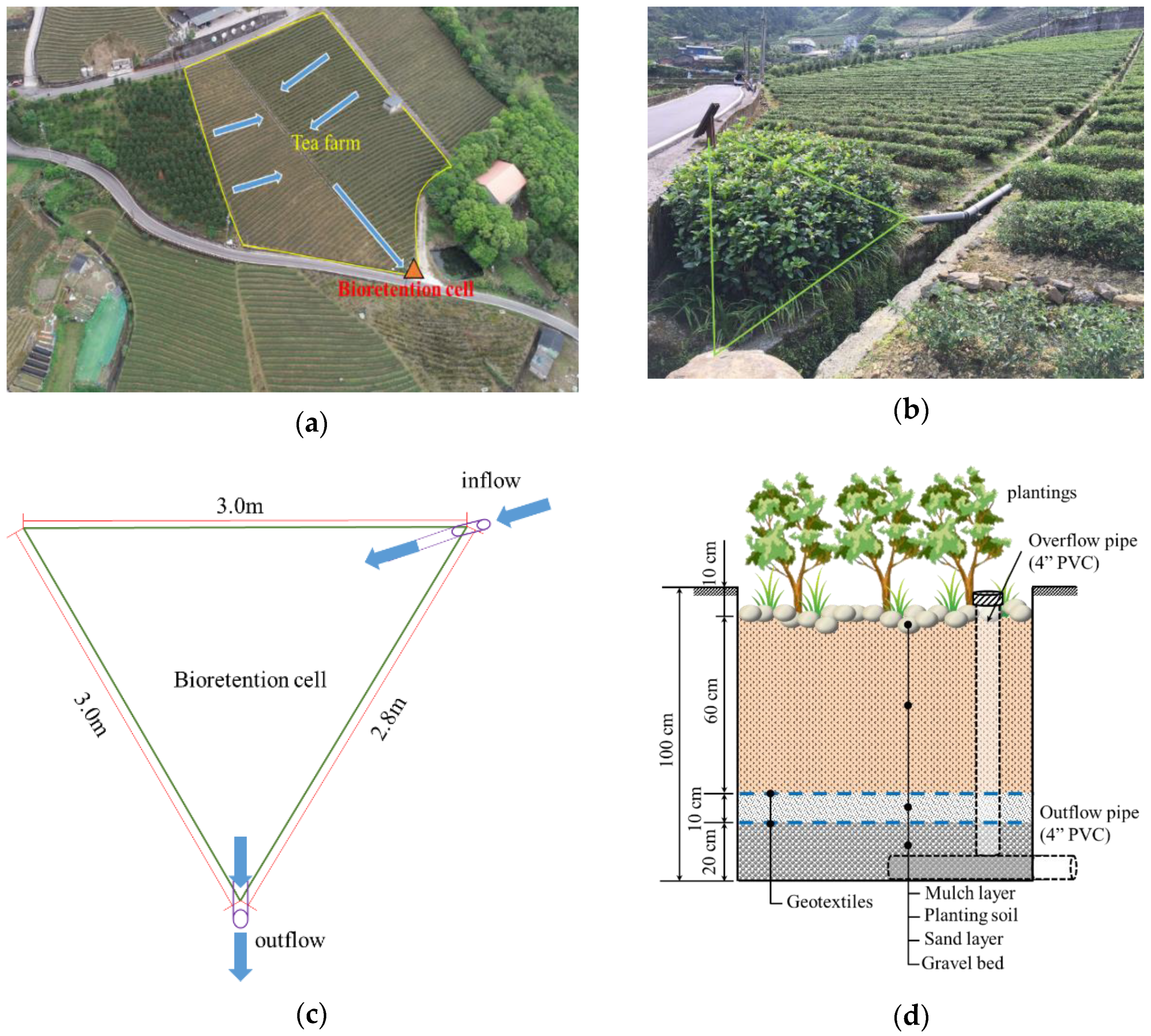
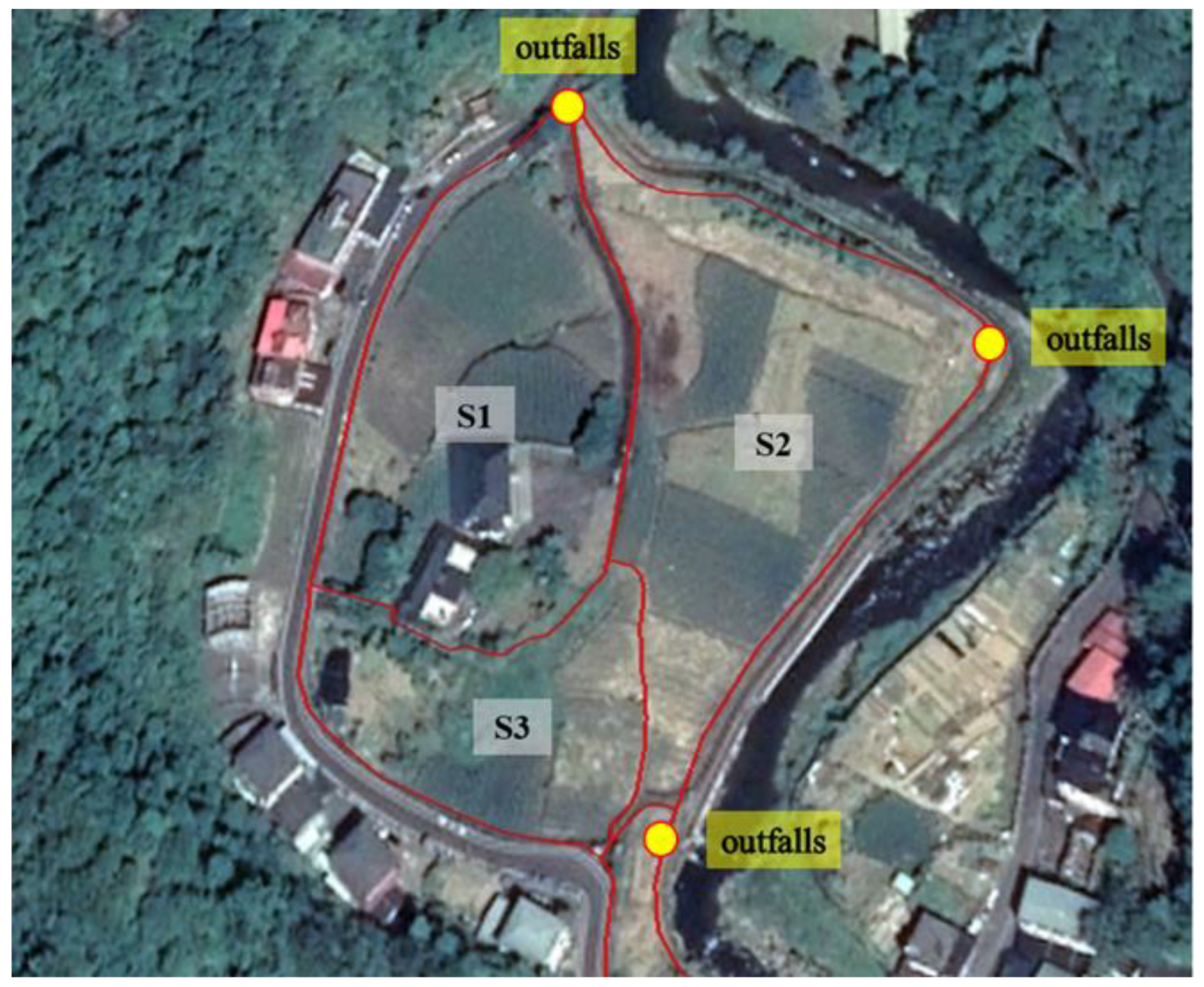
2.1. Case Study

The Jinggualiao stream in the Feitsui Reservoir (24.909097, 121.579736) was taken as a case study to present the idea of this study. Most domestic sewage within the watershed is well collected and treated. Therefore, nonpoint source pollution, especially tea farms, has become the largest potential pollution source of the reservoir. The total area of the reservoir watershed is 303 km2. The land use in the watershed is 96.6% forestland, 3% agricultural land, 1.2% artificial land, 4.1% water area and 1.1% other types. No industrial land uses, large commercial buildings or mining areas occur within the watershed. Three major inflow streams flow to the Feitsui Reservoir, and Jinggualiao stream is the target stream because of its relatively low water quality. The total area of the Jinggualiao watershed is 2350.96 ha, of which 93.9% is forest, 3.4% is agricultural land (mostly tea farms) and approximately 1% is for residential use. The land use of the Feitsui Reservoir and its inflow streams are shown in Figure 1. The average annual rainfall is 3500 mm, and the rainfall is concentrated from May to October, and affected by the early summer rainy and typhoon seasons.
The Feitsui Reservoir has very good water quality and from 1987 to 2018, the reservoir reached a eutrophic state only 3% of the time according to official data [25]. In recent years, the trophic level has been mesotrophic to oligotrophic. However, the detailed inflow streams sometimes exceed the required water quality standard in terms of total phosphorous (TP), especially the Jinggualiao stream. The TP concentration in the Jinggualiao stream from 2015 to 2018 is shown in Figure 2. The TP water quality standard is 20 μg/L for this reservoir and its streams. While the average TP concentration from 2015 to 2018 was 19.69 µg/L, which was less than the standard concentration, some of the observations did not meet the requirement.

2.2. Modeling Tool

The Storm Water Management Model (SWMM) model was used as a tool to evaluate the optimal size of bioretention cells for the watershed and tea farms. The SWMM includes a low impact development (LID) module and is capable of simulating the performance of different types of LID units. The SWMM can assess rainfall runoff for a watershed and help with drainage system design in urban and rural areas [26,27,28]. In addition, it can also simulate water quality from nonpoint source pollution. Therefore, it was used as a modeling tool to demonstrate the effectiveness of bioretention cells in reducing tea farm nonpoint source pollution. The details of SWMM and its mechanisms can be found on its open website (https://www.epa.gov/water-research/storm-water-management-model-swmm, accessed on 25 February 2022) and in its manual [29].
When applying the SWMM model, basic geographic data are needed, such as the digital elevation model (DEM), watershed boundary, stream distribution and land use. To transform the geographic data to SWMM inputs, the Better Assessment Science Integrating Point and Nonpoint Sources (BASINS) platform is helpful. BASINS is an integrated platform established by the USEPA to analyze required data as model inputs, and supports several water quality models, including SWMM. Therefore, BASINS was used to delineate subwatersheds, and the required geographic data were obtained for these subwatersheds. The details of model establishment are presented in the case study.

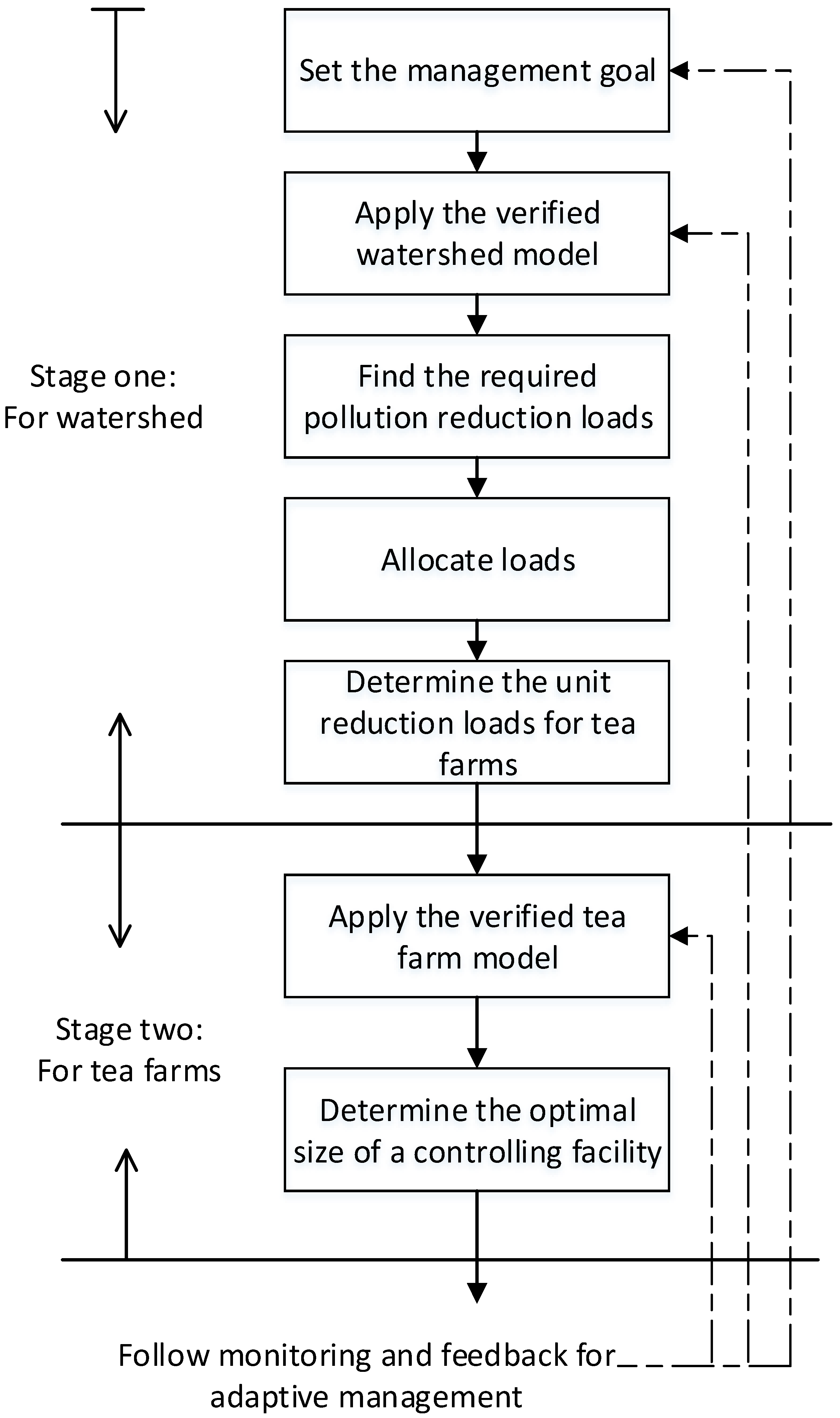
2.3. Optimization Process

The optimization process comprises two stages. The first stage is for the watershed scale. During this stage, the management goal is established and the carry capacity is determined; the management goal is also regarded as the required reduction load. The second stage is for the site scale. During this stage, the optimal LID facility size for each tea farm site is determined based on the unit reduction loads obtained from the first step. In the two-stage process, a total of seven steps are included. Steps 1 to 5 are for Stage 1 and Steps 6 to 7 are for Stage 2. In the two stages, two verified modeling tools are needed to provide quantitative data. The flow chart is shown in Figure 3. This flow is a universal process, and the modeling tools, the SWMM model and its LID module, are not limited to the use of this study. The core concept of the process is the connection between watershed-scale goals and site-scale design, and the idea of optimization is to accomplish the goal. The components of the process are explained below.
  • Step 1: Set the management goal
For any policy making, the first step is to decide the management goal. All subsequent policy design falls under this goal. In this step, as much background data as possible are needed to understand the state of the water, especially the water quality trend. Considering the current water quality, future changes in the environment and discussions with stakeholders, the management goal can be formed. A commonly used management goal for water quality is the legislated water quality standard, which is usually based on a concentration. A water quality concentration standard or the percentage of time that the water quality meets the standard (or achievement rate) can be used as the management goal. In addition, pollution loads, such as the Total Maximum Daily Loads (TMDL) policy in the U.S., are also good indicators. The choice of indicators can be determined by data sufficiency. If the number of observed water quality is few, the average concentration can be used. If long-term observed water quality data are available, then the achievement rate can be the indicator. If not only water quality but also water flow data are available, then the total reduction loads based on natural carry capacity would be a management goal.
  • Step 2: Apply the verified watershed model
A verified tool for demonstrating the complete water quality and discharge of a watershed is very important. Monitoring data are usually limited to specific locations and times. A modeling tool used after the verification process can serve as a useful tool to show more complete data about the water state. A quantitative tool to link the pollution sources, including the point and nonpoint sources, and the resulting water quality data are also necessary. Many watershed models are available to choose from, and a recommended rule for choosing a suitable one is that the model has been applied successfully and verified in similar regions and that the required data and model parameters are available for the specific case.
  • Step 3: Find the required reduction loads
This step uses the verified watershed model to calculate the required reduction loads under the management goal. With the verified modeling tool, it can simulate the water quality and discharge, and the total pollution loads can be obtained. Therefore, the total required pollutant loads under either the water quality standard concentration or the carry capacity can be calculated. The reduction loads required to match the management goal are then determined.
  • Step 4: Allocate loads
The required reduction loads of the watershed is then allocated to all pollution sources as their quantitative goal for control measures. Pollution sources include point sources and nonpoint sources. Load allocation should consider economic effectiveness such that point pollution sources are usually controlled before nonpoint sources. In this study, point sources had already been collected and treated by wastewater treatment plants; therefore, the study focused on nonpoint source pollution from tea farms. Tea farms are the obvious and major nonpoint source in the case study, and other pollution sources were not considered in this study.
  • Step 5: Determine the unit reduction loads for tea farms
This is the final output in the first stage. In the first stage, the unit reduction loads for tea farms (in this study, tea farms were the target pollution sources) is the total reduction in pollution loads divided by the total tea farm area, and the unit reduction load per tea farm area can be obtained and can serve as the target goal for the management of each tea farm. If more than one pollution source exists, the pollution load allocation needs more discussion, such as on effectiveness and equality.
  • Step 6: Apply the verified tea farm model
In this step, a verified tea farm model should be prepared. This model aims to be applied to site-scale tea farms, and the watershed-scale model in the first stage is not feasible. The site characteristics can be adjusted in the site-scale model. Because the site-scale model is different from the above watershed-scale model, the site-scale model needs to be tested through calibration and verification processes. When such a site-scale model is constructed, the unit reduction loads obtained in Step 5 can be used as the target loads for a tea farm.
  • Step 7: Determine the optimal size of a controlling facility
With the target allowable loads for a tea farm and the verified model, the next step is to find the optimal size of a controlling facility, I such as bioretention cells or another LID facility from the SWMM LID modules, required to match the target load in the tea farm case. This is an iterative process. An initial facility size is first input into the model and the loading difference before and after this facility design is checked. If the reduction load does not match the requirement, the size is adjusted until the required reduction load is achieved. The optimal size is based on the target load in this study and does not consider other factors, such as land space, cost and benefit or farmers’ will. The optimal size obtained from the procedure can serve as a specific and quantitative guide to know how many controlling facilities are needed. If space or budget is insufficient, the realistic size might be less than the optimal suggestion, and nonstructural Best Management Practices (BMPs) can be introduced to compensate for the required reduction loads. Nonstructural BMPs, such as increasing the frequency of cleaning or reducing the amount of fertilizers, are considered source management for reducing the pollution accumulations on the land surface. Nonstructural BMPs are not discussed in this study, but many official manuals, such as [30], are available.
The procedure demonstrates the optimal LID size for site-scale tea farms, and the optimal size is based on the required reduction loads allocated to tea farms. This is similar to the concept of the TMDL policy in the U.S. This procedure can be regarded as a universal procedure for linking the pollution sources within a watershed and the water quality in a receiving waterbody, and it can be used for different pollutants, sources or BMPs. In the procedure, a final step is the subsequent monitoring and feedback. Onsite monitoring data are crucial, and the data provide evidence for evaluating the performance of the policy. The observation data are very good feedback for rechecking the management goal or updating the simulation of the modeling tools.

3. Results and Discussion

3.1. Preparation of the Verified Model, Model Calibration and Verification

The SWMM model was applied to perform watershed-scale and site-scale modeling. The SWMM includes an LID module, which is very useful for assessing LID performance. In the two-stage optimization process, the watershed-scale model finds the total reduction loads and the site-scale model finds the optimal LID size required for each tea farm.
  • Watershed-scale model
The Jinggualiao stream is one of the streams into the Feitsui Reservoir, and its high TP concentration is of concern. The Jinggualiao watershed is divided into 7 subwatersheds according to their topography. The land use and DEM of the Jinggualiao watershed are shown in Figure 4. The rainfall data from the nearest official weather station were used as model inputs. Water discharge and water quality stations were used for observation data to verify the model simulations. The rainfall and flow discharge data were in the form of daily data, and the water quality data were in the form of monthly data.
The data from 2015 to 2016 were used for model calibration, and the data from 2017 were used for model verification. The model calibration and verification results are attached as supplemental files. Figure S1 shows the results of the flow simulations, and Figure S2 shows the results of the TP simulations, which are the target pollutants in this study. R2 and the mean absolute percentage error (MAPE) were used as the indicators to define the acceptable model results. When R2 is greater than 0.5 and the MAPE is less than 50%, the simulations are acceptable [31]. The verification results are summarized in Table S1.
2.
Site-scale model
The SWMM was verified for the Jinggualiao watershed in the first stage. In this stage, its feasibility for site-scale performance and its LID function must be tested. A 0.78 ha tea farm (24.918023, 121.681830) located within the Jinggualiao watershed was used to verify the site-scale simulations of the SWMM. On this tea farm, a bioretention cell with a 3.7 m2 area was built to treat runoff from the farm. Figure 5 shows a photograph of the site and its bioretention cell. The simulation results are shown in the supplemental files; please see Figure S3 and Table S3.

3.2. Optimization Results for the Jinggualiao Watershed (Step by Step)

The determination process and the verified models were applied to the Jinggualiao watershed and the case tea farm to demonstrate its application and results. The bioretention cell was used as the control facility in this study, but other control measures or combinations of several LID facilities can also be suggested in different cases.
  • Step 1: Set the management goal
The water quality standard for the Jinggualiao stream is classified as in Taiwan as Class A, which is used for public drinking water and requires the highest water quality. The TP concentration standard was equal to or less than 20 µg/L. For reservoirs in Taiwan, phosphorous, rather than nitrogen, is the pollutant of concern [23,24]. As one of the upstream areas of the Feitsui Reservoir, the average TP concentration of the Jinggualiao was approximately 18.44 μg/L, which was higher than that of other streams. However, the average TP concentration of the Jinggualiao watershed was less than the TP standard requirement, 20 μg/L. Not all data were less than the standard value. Using the achievement rate to indicate water quality, the average achievement rate was only 58.3% (Table 1). Therefore, the achievement rate is a better indicator than the average TP concentration to set as the management goal for this case study.
  • Step 2: Apply the verified watershed model
The verified watershed model aims to link pollution exposure from the watershed and the resulting water quality. From Step 1, the current water quality status was available, and the achievement rate was selected as the management goal indicator. However, the observed data were collected once a month, and an annual trend was hardly seen. When the results from the verified model were used, the daily water quality could be used to supplement the management goal data. The comparison of observations and simulations of water quality are summarized in Table 2. The achievement rates were quite different, 58.3% from the observations and 79.93% from the simulations. This is because one was based on monthly data while the other used daily data. Because most water quality parameters were below the standard, the percentage that achieves the requirement would increase. In the following steps, the modeling tools use this information; therefore, the management goals were set to 85% and 90% of the TP concentration achievement rate based on the simulation results. These goals were then regarded as the short-term and long-term management goals for the Jinggualiao stream.
  • Step 3: Find the required reduction loads
After setting the TP achievement rate to 85% and 90%, the next step was to find the required reduction loads. In this step, a trial process is needed. In the SWMM model, users can set a unit of a bioretention cell and denote how many of these facilities are placed within the watershed. The model will generate runoff discharge and water quality after LID placement. Therefore, an initial area of bioretention could be set, and a trial process could be used to determine the number of facilities needed to reach the management goal.
Figure 6 shows the trial process, in which the TP concentration was simulated under different areas of bioretention cells denoted along the Jinggualiao stream. With every test, the achievement rate was calculated. According to the figure, the peak concentration was obviously reduced with increasing bioretention cell area, implying the effectiveness of this control facility on nonpoint source pollution. For example, in Table 3, 300 m2 of bioretention cells increases the achievement rate from 79.93% (current) to 83.95%, and 350 m2 and 600 m2 will reach the goals of 85% and 90%, respectively. The simulated water flow and water quality can be used to calculate the loads. The current average TP load per year is 534.74 kg. The reduction load needed is 16.52 kg/year to match the 85% goal, and 26.38 kg/year to match the 90% goal. In this step, the reduction loads and the required area of the bioretention cells to reduce the loads were obtained.
  • Step 4: Allocate loads
The reduction loads should be allocated to all pollution sources, and they should be allocated to point sources prior to nonpoint sources due to the cost issue. However, in this case, the point sources had already been well controlled. As a result, the required reduction loads were allotted to nonpoint sources. In the Jinggualiao watershed, tea farms are the dominant nonpoint sources of pollution, and the required reduction loads were allocated to these tea farms.
  • Step 5: Determine the unit reduction loads for tea farms
The tea farms are mostly located downstream in the Jinggualiao watershed, where the total area of the tea farms is 61.18 ha. If the total reduction loads of TP are allocated to these tea farms, the unit reduction load is 270 g/ha-year for the 85% goal and 326 g/ha-year for the 90% goal. These unit reduction loads do not consider the specific properties of each tea farm and regard their impact on stream water quality as equal. This value is critical and serves as the management goal of the tea farms for the subsequent control measure design. The unit TP reduction load for the tea farms are summarized in Table 4.
  • Step 6: Apply the verified tea farm model
When the unit TP reduction loads were obtained, the control measures for each tea farm were designed based on this requirement. In this study, bioretention cells were selected as the control measure, and other BMPs were not considered. A verified site-scale model tool, the SWMM model with the LID module, was used. Here, one tea farm was presented to show its application.
The demonstrated tea farm, which has three drainage systems and three outflows, is shown in Figure 7. The area of this tea farm is 1.987 ha, and the slope ranges from 6 to 10%. According to the unit reduction loads, this tea farm must reduce 534 g of TP per year to reach the 85% goal and reduce 648 g of TP per year to achieve the 90% goal.
  • Step 7: Determine the optimal size of a controlling facility
This example tea farm has three subwatersheds; thus, the runoff from the three subwatersheds should be calculated separately. This step requires time to determine the number of bioretention cells needed to match the required TP loads. In the model, the size of the bioretention unit is set, including its vertical properties, and the process is iterative. Taking one of the subwatersheds as an example, the area of the S1 subwatershed is 0.890 ha, and the required TP reduction loads are 240 and 290 g/y for the 85% and 90% goals, respectively. Table 5 shows the simulation results. When the bioretention cell area was set to 3 m2, the reduction load was 62 g/y, less than the required loads of 240 g/y and 290 g/y. After applying the process and interpolation, areas of 11.8 and 14.3 m2 were found to achieve the required loads for the S1 subwatershed. Following this process, the optimal area of the bioretention cells for the other two subwatershedswere were obtained (Table 6). The final optimal LID size for this tea farm is 26 m2 to achieve the 85% goal and 32 m2 to achieve the 90% goal. This is very useful information for control policy design, and the required TP reduction and suggested LID size were determined.
In addition to this tea farm case study, the optimization process was applied to 30 other tea farms in this watershed. Reduction goals and individual models were established for each tea farm. Due to the different sizes and geographical characteristics, the optimal sizes of bioretention cells were different. The average area of the bioretention cells was 13 m2 for each hectare of tea farm.

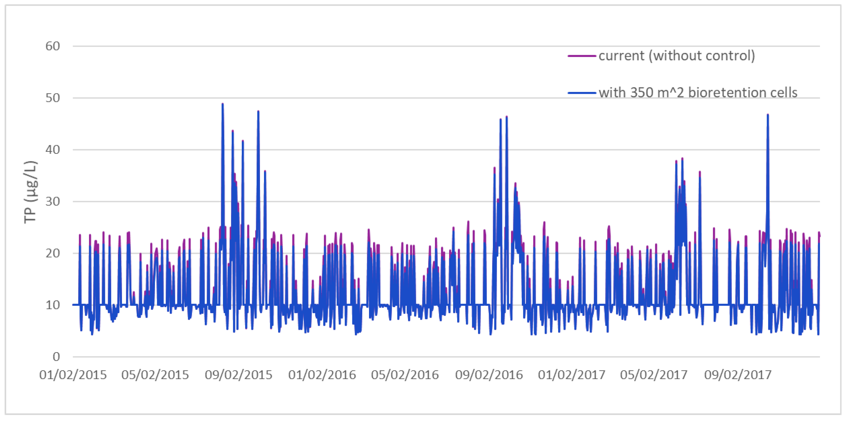
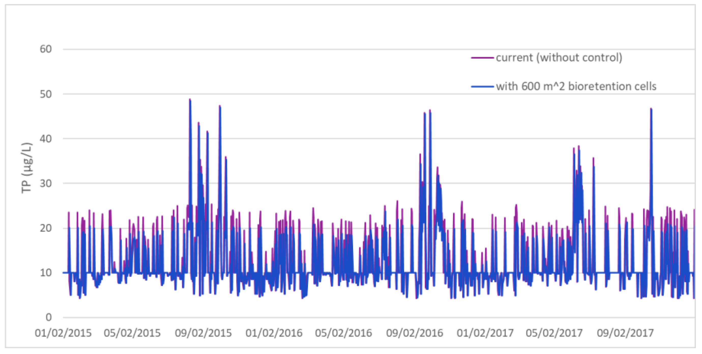
3.3. Expected Water Quality Improvement Using Bioretention Cells

Following the optimization process, 350 m2 and 600 m2 of bioretention cells are needed to reach the goals of 85% and 90% of the water quality achievement rate in the Jinggualiao stream. The relationship between the area of bioretention cells and the water achievement rate is shown in Figure 8. Notably, the slopes before and after 250 m2 were different. After 250 m2, the effectiveness of the bioretention cell was better than that at less than 250 m2, which means that every 1 m2 of bioretention cell resulted in a better water quality achievement rate. This is because the achievement rate is accounted for by a TP concentration of less than 20 μg/L. When bioretention cells or other onsite runoff treatment facilities are built, the water quality is expected to improve in wet weather. The improved water quality concentration might not be as low as the required standard equally. When the bioretention cell area is sufficient, the quantity of improved water quality that is lower than the standard will increase nonlinearly. This implies that small control facilities might not perform as expected, but the gradual accumulation of work on runoff control is worthwhile and will have satisfactory results.
A 1 m2 bioretention cell can reduce TP loads by 55 g/year according to the results of the watershed-scale model; however, this value is not recommended for use at each tea farm site. In the Jinggualiao watershed, the conditions of tea farms are quite different. Tea farms are located on either flat land or sloping fields. The slope and water routes are very different on different tea farms; therefore, the effectiveness of bioretention cells is not equal at each site. For this reason, a site-scale model is required to determine the optimal control size for the tea farms. For example, the results of the tea farm case study (Table 6) show that a 1 m2 bioretention cell reduces TP loads by approximately 20.5 g/year, which is much less than the average value resulting from the whole watershed. To provide detailed information for each tea farm, the site-scale model is helpful for assessing the water collection route, the location of the control facility, and the optimal size for reaching the management goal.

4. Conclusions

In this study, a process was established to link a watershed management goal and a site-scale control policy. Nonpoint source pollution relies on onsite control methods, either structural or nonstructural measures. However, what level of control measures is needed for site-scale management or what size of structural measures should be designed is difficult to determine. From the process presented in this study, the optimal size of bioretention cells for a tea farm can be determined, and the optimal size is based on the watershed management goal. In addition to the team farm presented, the process was applied to more than 30 tea farms in this watershed. A 1 m2 bioretention cell could reduce TP loads by 55 g/year, and an average of 13 m2 bioretention cells were suggested for 1 ha tea farm to match the 85% goal. When considering the loss from delivery, which means that pollutants exported from tea farms will not all reach waterbodies, a LID area smaller than 13 m2/ha might be used. At least 10 m2 of bioretention cells for each 1 ha tea farm is suggested. Therefore, a ratio of 1 to 1000 for the area of bioretention cells to the area of a tea farm is recommended as a control rule. Considering the onsite properties of tea farms, the optimal size might be different. The SWMM model with the LID module is a useful tool. Before application to different cases, model calibration and verification are necessary. Once the model is verified, the determination process can be used for different cases and different LID facilities.
This process was applied to the Jinggualiao watershed for three years, and a total of 89 m2 of bioretention cells distributed in 49 tea farms were built. While applying this process to real cases, realistic problems occurred: The land area might not be sufficient, or the landowners might not be able to provide the area for building control facilities. In these cases, nonstructural measures such as reducing fertilizer application are needed. The unit reduction loads were determined for tea farms, and they were 270 g/ha-year for the 85% goal and 326 g/ha-year for the 90% goal. If structural facilities are insufficient, a level of nonstructural measures can also be designed based on unit reduction loads. Therefore, with a quantitative determination process, policy measures can be better assessed and designed.

Supplementary Materials

The following supporting information can be downloaded at: https://www.mdpi.com/article/10.3390/app12052661/s1, Figure S1: Flow simulation results. The upper part shows flow calibration using data from 2015 to 2016, and the bottom part shows flow verification using data from 2017. Figure S2: TP simulation results. The upper part shows TP calibration using data from 2015 to 2016, and the bottom part shows TP verification using data from 2017. Figure S3: The simulation results at the site-scale, including runoff discharge, TP concentration and TP concentration in the LID outflow. Table S1: The results of SWMM model calibration and verification for the Jinggualiao stream watershed. Table S2: The calibrated model parameters for the watershed-scale SWMM model. Table S3: The calibrated model parameters and dimensions of the bioretention cell used in the model.

Author Contributions

Conceptualization, C.-F.C. and C.-C.H.; methodology, C.-F.C. and C.-C.H.; software, C.-F.C.; validation, C.-C.H. and H.-F.L.; resources, H.-F.L.; writing—original draft preparation, C.-F.C.; writing—review and editing, C.-F.C. and C.-C.H.; supervision, C.-C.H.; project administration, H.-F.L.; funding acquisition, H.-F.L. All authors have read and agreed to the published version of the manuscript.

Funding

This research was funded by Taipei Water Management Office, Water Resources Agency, grant number MOEAWRA1090095.

Institutional Review Board Statement

Not applicable.

Informed Consent Statement

Not applicable.

Data Availability Statement

Not applicable.

Conflicts of Interest

The authors declare no conflict of interest. The funders had no role in the design of the study; in the collection, analyses, or interpretation of data; in the writing of the manuscript, or in the decision to publish the results.

Acronyms

BASINSBetter Assessment Science Integrating Point and Nonpoint Sources platform
BMPsBest Management Practices
DEMDigital elevation model
LIDLow impact development
MAPEMean absolute percentage error
SWMMStorm Water Management Model
TMDLTotal Maximum Daily Loads
TPTotal phosphorous

References

  1. Romstad, E. Team Approaches in Reducing Nonpoint Source Pollution. Ecol. Econ. 2003, 47, 71–78. [Google Scholar] [CrossRef]
  2. Dowd, B.M.; Press, D.; Los Huertos, M. Agricultural Nonpoint Source Water Pollution Policy: The Case of California’s Central Coast. Agric. Ecosyst. Environ. 2008, 128, 151–161. [Google Scholar] [CrossRef]
  3. Loucks, D.P.; Van Beek, E. Water Resource Systems Planning and Management: An Introduction To Methods, Models, and Applications; Springer: Cham, Switzerland, 2017. [Google Scholar]
  4. Rong, Q.; Cai, Y.; Chen, B.; Shen, Z.; Yang, Z.; Yue, W.; Lin, X. Field Management of A Drinking Water Reservoir Basin Based on The Investigation of Multiple Agricultural Nonpoint Source Pollution Indicators in North China. Ecol. Indic. 2018, 92, 113–123. [Google Scholar] [CrossRef]
  5. Xiang, C.Y.; Wang, Y.; Liu, H.W. A Scientometrics Review on Nonpoint Source Pollution Research. Ecol. Eng. 2017, 99, 400–408. [Google Scholar] [CrossRef]
  6. Park, M.; Choi, Y.S.; Shin, H.J.; Song, I.; Yoon, C.G.; Choi, J.D.; Yu, S.J. A Comparison Study of Runoff Characteristics of Non-Point Source Pollution from Three Watersheds in South Korea. Water 2019, 11, 966. [Google Scholar] [CrossRef] [Green Version]
  7. Baker, L.A. Introduction to nonpoint source pollution in the United States and prospects for wetland use. Ecol. Eng. 1992, 1, 1–26. [Google Scholar] [CrossRef]
  8. Dzikiewicz, M. Activities in nonpoint pollution control in rural areas of Poland. Ecol. Eng. 2000, 14, 429–434. [Google Scholar]
  9. Liu, R.M.; Wang, J.W.; Shi, J.H.; Chen, Y.X.; Sun, C.C.; Zhang, P.P.; Shen, Z.Y. Runoff characteristics and nutrient loss mechanism from plain farmland under simulated rainfall conditions. Sci. Total Environ. 2014, 468, 1069–1077. [Google Scholar] [CrossRef]
  10. Kim, H.C.; Yoon, C.G.; Son, Y.K.; Rhee, H.P.; Lee, S.B. Effects of Open Water on The Performance of A Constructed Wetland for Nonpoint Source Pollution Control. Water Sci. Technol. 2010, 62, 1003–1012. [Google Scholar] [CrossRef]
  11. Jia, Z.; Tang, S.; Luo, W.; Hai, Y. Water Quality Improvement through Five Constructed Serial Wetland Cells and Its Implications on Nonpoint-Source Pollution Control. Hydrol. Sci. J. 2016, 61, 2946–2956. [Google Scholar] [CrossRef]
  12. Diaz, F.J.; O’Geen, A.T.; Dahlgren, R.A. Agricultural Pollutant Removal by Constructed Wetlands: Implications for Water Management and Design. Agric. Water Manag. 2012, 104, 171–183. [Google Scholar] [CrossRef]
  13. Roy-Poirier, A.; Champagne, P.; Filion, Y. Bioretention Processes for Phosphorus Pollution Control. Environ. Rev. 2010, 18, 159–173. [Google Scholar] [CrossRef]
  14. Goh, H.W.; Lem, K.S.; Azizan, N.A.; Chang, C.K.; Talei, A.; Leow, C.S.; Zakaria, N.A. A Review of Bioretention Components and Nutrient Removal under Different Climates-Future Directions for Tropics. Environ. Sci. Pollut. Res. 2019, 26, 14904–14919. [Google Scholar] [CrossRef]
  15. Osman, M.; Yusof, K.W.; Takaijudin, H.; Goh, H.W.; Malek, M.A.; Azizan, N.A.; Ghani, A.A.; Abdurrasheed, A.S. A Review of Nitrogen Removal for Urban Stormwater Runoff in Bioretention System. Sustainability 2019, 11, 5415. [Google Scholar] [CrossRef] [Green Version]
  16. Sheng, L.T.; Zhang, Z.; Xia, J.; Liang, Z.; Yang, J.; Chen, X.A. Impact of Grass Traits on The Transport Path and Retention Efficiency of Nitrate Nitrogen in Vegetation Filter Strips. Agric. Water Manag. 2021, 253, 106931. [Google Scholar] [CrossRef]
  17. Lintern, A.; McPhillips, L.; Winfrey, B.; Duncan, J.; Grady, C. Best Management Practices for Diffuse Nutrient Pollution: Wicked Problems across Urban and Agricultural Watersheds. Environ. Sci. Technol. 2020, 54, 9159–9174. [Google Scholar] [CrossRef]
  18. Yang, Y.S.; Wang, L. A Review of Modelling Tools for Implementation of the EU Water Framework Directive in Handling Diffuse Water Pollution. Water Resour. Manag. 2010, 24, 1819–1843. [Google Scholar] [CrossRef] [Green Version]
  19. Li, Z.; Luo, C.; Jiang, K.; Wan, R.; Li, H. Comprehensive Performance Evaluation for Hydrological and Nutrients Simulation Using the Hydrological Simulation Program-Fortran in a Mesoscale Monsoon Watershed, China. Int. J. Environ. Res. Public Health 2017, 14, 1599. [Google Scholar] [CrossRef] [Green Version]
  20. Yazdi, J.; Moridi, A. Interactive Reservoir-Watershed Modeling Framework for Integrated Water Quality Management. Water Resour. Manag. 2017, 31, 2105–2125. [Google Scholar] [CrossRef]
  21. Chen, C.F.; Wu, Y.R.; Lin, J.Y. Applying a Watershed and Reservoir Model in an Off-Site Reservoir to Establish an Effective Watershed Management Plan. Processes 2019, 7, 484. [Google Scholar] [CrossRef] [Green Version]
  22. Shoemaker, L.; Dai, T.; Koenig, J.; Hantush, M. TMDL Model Evaluation and Research Needs: National Risk Management Research Laboratory; US Environmental Protection Agency: Washington, DC, USA, 2005. [Google Scholar]
  23. Environment Protection Administration, Executive Yuan, R.O.C (Taiwan). A Study for Nutrients Reduction Strategies for Eutrophication Potential Reservoirs; EPA-105-G103-02-A073; Environment Protection Administration, Executive Yuan, R.O.C: Taipei, Taiwan, 2016. (In Chinese) [Google Scholar]
  24. Environment Protection Administration, Executive Yuan, R.O.C (Taiwan). A Study of Sustainable Water Quality Management for Eutrophication Potential Reservoir; EPA-106-U1-02-A096; Environment Protection Administration, Executive Yuan, R.O.C: Taipei, Taiwan, 2017. (In Chinese) [Google Scholar]
  25. The Water Quality Data of the Feitsui Reservior. Available online: https://www.feitsui.gov.taipei/News.aspx?n=3EAD35A938E561D5&sms=F34446182ADE1B69 (accessed on 25 February 2022).
  26. Temprano, J.; Arango, Ó.; Cagiao, J.; Suárez, J.; Tejero, I. Stormwater Quality Calibration by SWMM: A Case Study in Northern Spain. Water SA 2005, 32, 55–63. [Google Scholar] [CrossRef] [Green Version]
  27. Moynihan, K.P.; Vasconcelos, J. SWMM Modeling of a Rural Watershed in the Lower Coastal Plains of the United States. J. Water Manag. Model. 2014, 22. [Google Scholar] [CrossRef] [Green Version]
  28. Talbot, M.; McGuire, O.; Olivier, C.; Fleming, R. Parameterization and Application of Agricultural Best Management Practices in A Rural Ontario Watershed Using PCSWMM. J. Water Manag. Model. 2016, 24. [Google Scholar] [CrossRef] [Green Version]
  29. Rossman, L.A. Storm Water Management Model User’s Manual Version 5.1; U.S. Environmental Protection Agency: Washington, DC, USA, 2015. [Google Scholar]
  30. The Pennsylvania Stormwater Best Management Practices Manual. Available online: http://www.stormwaterpa.org/from-the-foreword.html (accessed on 25 February 2022).
  31. Moriasi, D.N.; Arnold, J.G.; Van Liew, M.W.; Bingner, R.L.; Harmel, R.D.; Veith, T.L. Model Evaluation Guidelines for Systematic Quantification of Accuracy in Watershed Simulations. Trans. ASABE 2007, 50, 885–900. [Google Scholar] [CrossRef]
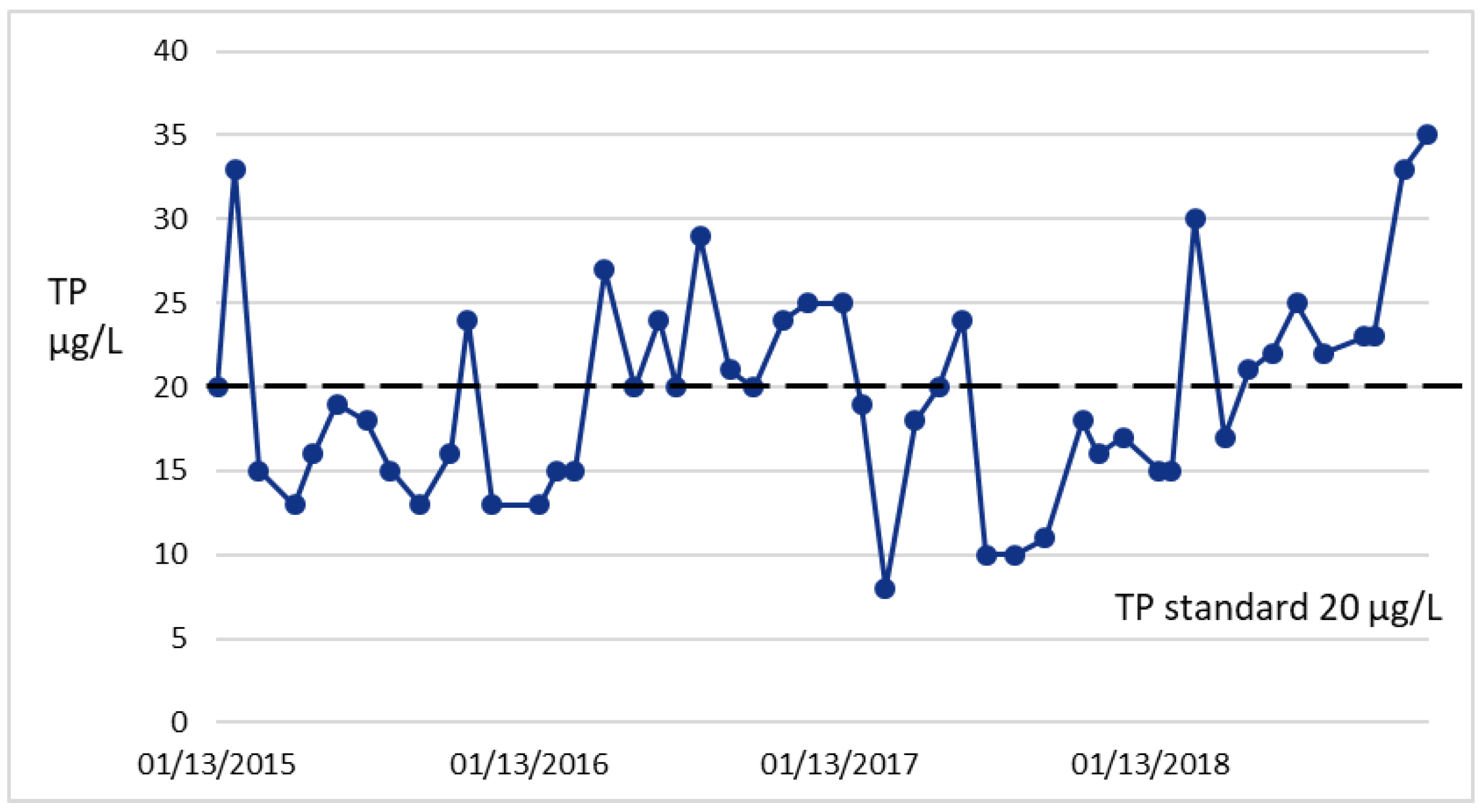
Figure 1. The land use and main streams of the Feitsui Reservoir watershed.
Applsci 12 02661 g001
Figure 2. Total phosphorous (TP) concentration of the Jinggualiao stream from 2015 to 2018.
Applsci 12 02661 g002
Figure 3. The two-stage optimization process for watershed and tea farm management.
Applsci 12 02661 g003
Figure 4. The land use and DEM of the Jinggualiao watershed.
Applsci 12 02661 g004
Figure 5. The tea farm site and its bioretention cell used for verification of the site-scale SWMM LID module. (a) The boundary of the studied tea farm, (b) the location of bioretention cell in the downstream of the tea farm, (c) the dimension of the bioretenrion cell and (d) the profile section of the bioretention cell.
Applsci 12 02661 g005
Figure 6. TP simulation results using different areas of bioretention cells. The upper panel shows 350 m2 of bioretention cells, and the bottom panel shows 600 m2 of bioretention cells.
Applsci 12 02661 g006aApplsci 12 02661 g006b
Figure 7. Example tea farm within the Jinggualiao watershed. This tea farm has three subwatersheds and 3 outfalls.
Applsci 12 02661 g007
Figure 8. The relationship between the area of bioretention cells and the water quality achievement rate in the Jinggualiao stream.
Applsci 12 02661 g008
Table 1. The average TP concentration and the achievement rate of the Jinggualiao stream from 2015 to 2017.
YearTP Concentration (μg/L)
(n = 12 per Year)
Achievement Rate
(The Percentage of Data Less than 20 μg/L)
201517.9275.0%
201621.0825.0%
201716.3375.0%
Average18.4458.3%
Table 2. Comparison of the observed and simulated average TP concentrations and the achievement rate from 2015 to 2017.
YearTP Concentration (μg/L)Achievement Rate
(The Percentage of Data Less than 20 μg/L)
Observations
(n = 12 per Year)
Simulations
(n = 365 per Year)
Observations
(n = 12 per Year)
Simulations
(n = 365 per Year)
201517.9215.2575.0%82.14%
201621.0812.0525.0%79.23%
201716.3313.0975.0%78.43%
Average18.4413.4658.3%79.93%
Table 3. The achievement rate of TP under different areas of bioretention cells placed within the watershed.
YearBioretention Cell Area (m2)
50100200300350375400450600
201583.2%84.1%84.6%85.44%85.2%86.81%87.09%87.64%90.4%
201679.8%80.3%82.2%84.70%87.4%87.98%88.25%89.62%91.3%
201778.4%79.1%80.4%81.70%83.0%82.68%83.66%84.97%88.2%
Average80.5%81.2%82.4%83.95%85.2%85.82%86.33%87.41%90.0%
Table 4. The unit TP reduction loads of tea farms required to match the target goal: 85% and 90% water quality achievement rates.
Achievement RateAverage TP Loads (kg/Year)Required Reduction Load (kg/Year)Unit Reduction Load for Tea Farms (g/ha)
79.93% (current)534.74--
85%518.2216.52270
90%508.3626.38326
Table 5. Determination process for the S1 subwatershed in the case tea farm.
Bioretention Cell Area (m2)TP Loads with Bioretention Cells (g/y)Reduction Loads (g/y)Reduction Rate (%)
32055622.9%
619921265.9%
919311868.8%
12187124711.6%
18175636217.1%
Table 6. The optimal LID size suggested for the tea farm case study.
Tea Farm Case StudyUnitS1S2S3Total
Areaha0.8900.5800.5171.987
Original TP exportg/y2118138112424741
Required TP reduction loads for 85% goalg240157140537
Required TP reduction loads for 90% goal290189169648
The optimal LID size for 85% goalm211.87.76.726.2
The optimal LID size for 90% goal14.39.48.231.8
Publisher’s Note: MDPI stays neutral with regard to jurisdictional claims in published maps and institutional affiliations.

