Arc Modeling and Kurtosis Detection of Fault with Arc in Power Distribution Networks

Abstract

In power distribution networks, there are many practical fault cases such as high impedance faults, faults and so on. Especially when the faults with electric arc persist, it is dangerous for human beings and circumstances. Nevertheless, it is difficult to classify faults due to various customer load conditions or the presence of distributed energy resources. In this paper, we propose a new mathematical arc model based on experimental event data. For implementing the arc phenomenon, wet gravel was used as a contact conductor after the fault. The experimental results validate the arc transient model. Then, the simulations were performed to verify the success of arc modeling using Kizilcay’s arc model as a comparison method. Finally, we developed a fault detector using the kurtosis detection method, and power system simulations were conducted to evaluate fault detection performance using Matlab/Simulink.

1. Introduction

In power distribution networks, it is extremely important to safely supply power under various fault conditions. Specifically, it is difficult to detect faults in a power distribution network because factors such as load and distributed energy resources exist [1,2,3]. When the faults persist, it leads to dangerous circumstances for individuals because the faults are typically high voltage or high current. Therefore, it is necessary to develop an effective detection method for determining whether to continuously supply power.

Over the past few decades, various approaches have been examined to remedy these problems [4,5,6,7,8,9,10,11,12,13,14,15]. Typically, harmonic patterns are utilized to capture fault characteristics such as magnitude and angles or harmonics [4,5,6]. The stator-ground fault location method based on third-harmonic measures was proposed in [4,5]. Various harmonics in current waveforms were used to design a general purpose model for representing a high impedance fault [6]. In [7], a new approach for fault detection was developed based on the energy variation of the low harmonic orders obtained by the Stockwell transform. In [8], a nonlinear equivalent model and detection algorithm were developed by analyzing odd harmonics amplitudes. In addition, there are many signal processing methodologies, including the Kalman filter-based method, wavelet transform, and short-time Fourier transform [9,10,11,12]. In [9], a Kalman filter-based algorithm was developed for series arc fault detection. In [10,11,12], the time domain reflectometry-based fault location method using a wavelet decomposition was proposed. Recently, various methods based on machine learning have been proposed [13,14,15]. A hierarchical classification and machine learning method were designed to detect and classify the line-to-ground and line-to-line faults in PV systems in [13]. As a deep learning method, the convolutional autoencoder framework for HIF detection was proposed in [14]. The useful features with advanced machine learning methods were extracted in [15].

Unfortunately, the aforementioned methods were developed without considering arc modeling, which inevitably occurs in actual fault situations. There are many fault situations in which power distribution lines are disconnected or are energized with other conductors. When a distribution line becomes disconnected, an arc can frequently occur along with electrical breakdown because the disconnected distribution line is in contact with other conductors. An arc exhibits an instantaneous low current with respect to high contact pressure. Hence, it can be easily ignited when it comes in contact with other conductors. Therefore, based on the type of conductor it contacts, an arc can cause damage in the form of electric shocks and economic losses from wildfires.

Many methods have been examined from different perspectives for arc detection and arc modeling. However, most of the previous methods were performed based on the existing mathematical arc models without considering practical arc fault events. It is challenging to model an arc because the arc fault waveforms vary based on the contacted (energized) conductor. Additionally, given that an arc is instantaneously created, conventional methods, such as unbalanced voltage/current amplitude detection, angle different detection, and n-th harmonic detection, are not effective.

This paper contributes to developing an arc model of fault in the power distribution network. Modeling requires experimental data to fulfil its equations and their parameters. Hence, an experimental setup is implemented to establish a single-phase fault with a mathematical arc model in a 3-phase distribution system. To analyze arc phenomenon, phase voltage and phase current are measured via remote terminal units (RTUs) at different locations. The experiment results are used to model the arc. The arc phenomenon is modeled using linear and nonlinear functions after analyzing the arc regions based on the experimental waveforms. Then, a verification process using simulations is conducted to evaluate similarity between the mathematical arc model and arc phenomenon in experimental results. Furthermore, the fault detection method based on kurtosis detector is developed to detect the fault with arc. Additionally, power system simulations are performed to confirm the effectiveness of the proposed arc detection algorithm.

The main contributions of this paper are as follows:

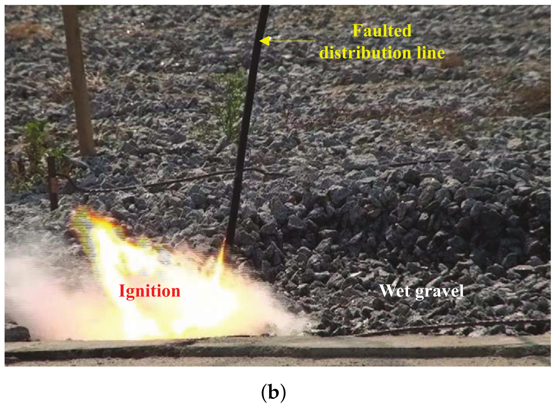
• Fault with arc was experimentally implemented for arc waveform analysis.
• New arc model was mathematically designed by solely using arc voltage.
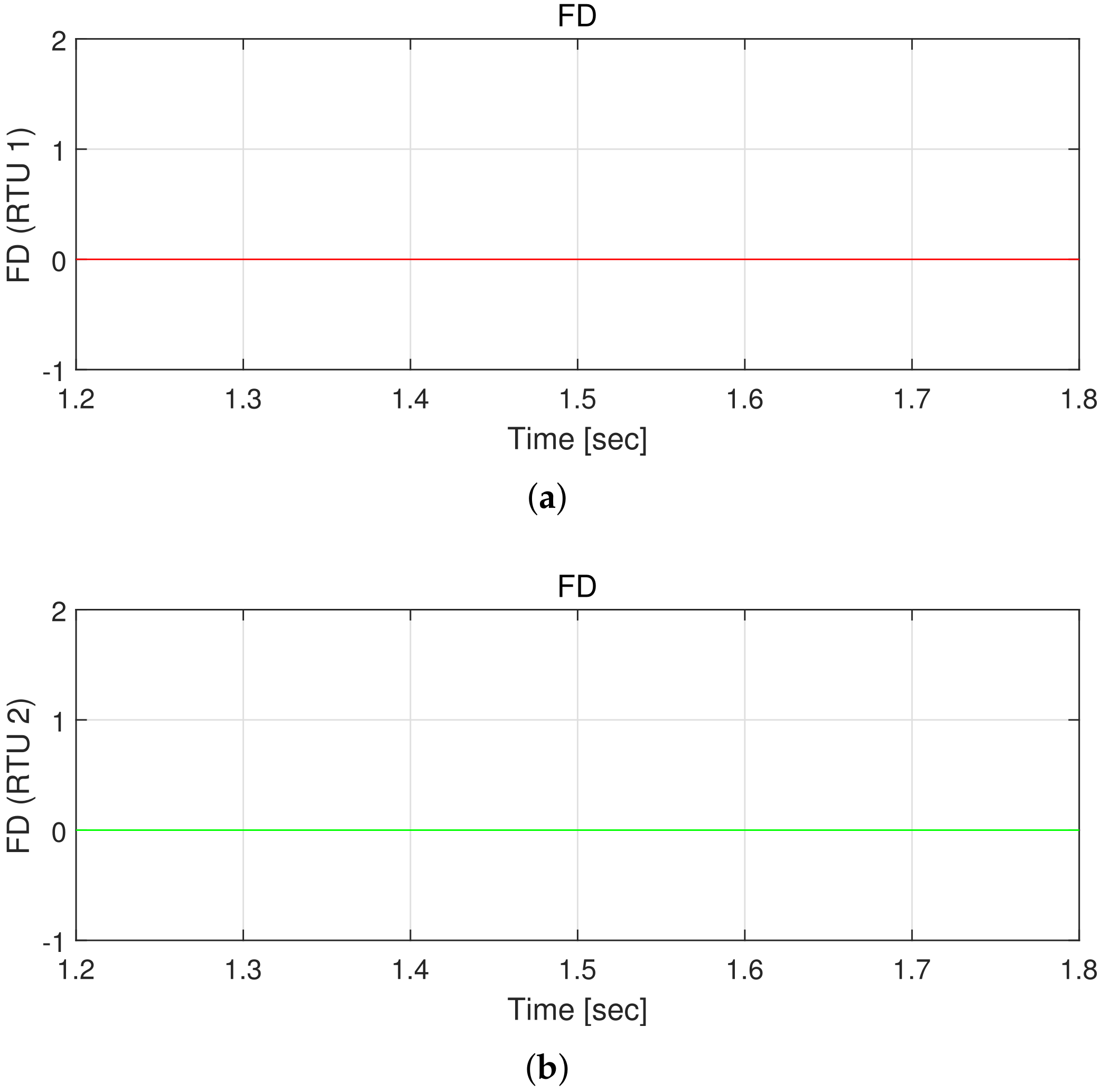
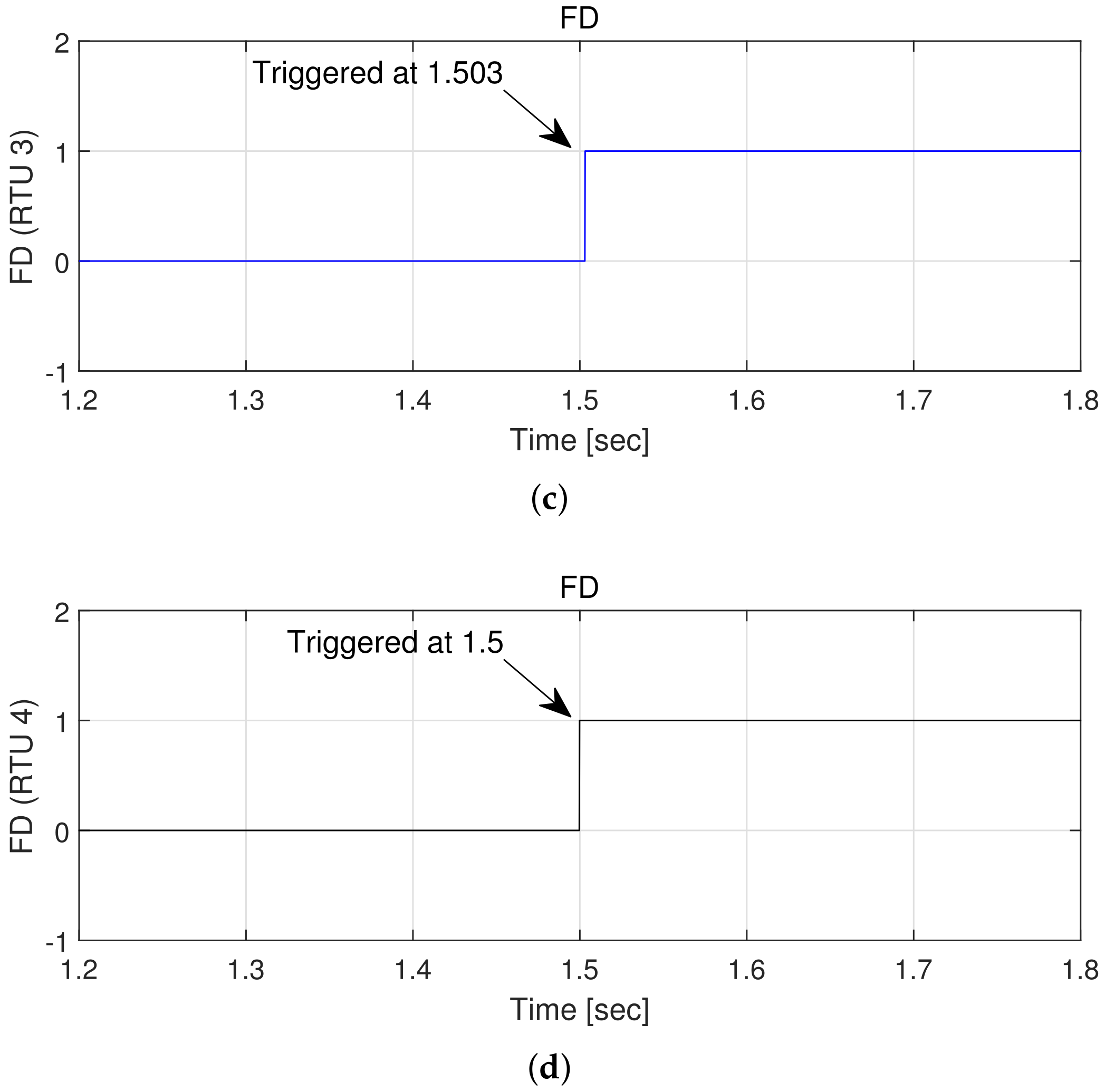
• Fault detector based on kurtosis detection algorithm was developed and detection performance was validated using simulation.

This paper is organized as follows. Section 2 explains practical problems for open fault with arc and shows both the experimental results and waveform analysis to analyze the arc phenomenon. The design procedure of the proposed arc model is provided in Section 3. We develop a fault detection algorithm and conduct simulations to show the effectiveness of the fault detection performance in Section 4 and Section 5.

2. Experimental Work and Arc Waveform Analysis

2.1. Problem Statement

Several mathematical models have been used for describing the arcs. Many models are used for circuit breaker arcs [16,17] and several of these models have been applied to long arcs or arcing faults [18,19]. The most popular rules depend on thermal equilibrium. Hence, the thermal model has the longest history of dynamic arc models since the introduction of the first description of arc conductivity in the form of a first order differential equation by Cassie 1939 and Mayr 1943 [1].

Even if the thermal model increases a model’s validity and reduces the computation burden, two concerns still remain for an arc model. First, given that in the previous methods the time varying arc conductance was calculated using the phase current, the variation in phase current is inevitably sensitive to the customer load. Second, phase voltage and phase current can potentially not be in-phase because there are various types of loads such as inductive loads and capacitive loads. Consequently, when the phase voltage and phase current are not in-phase, it is difficult to calculate negative arc conductance in the previous methods by using the phase current as an input of the model.

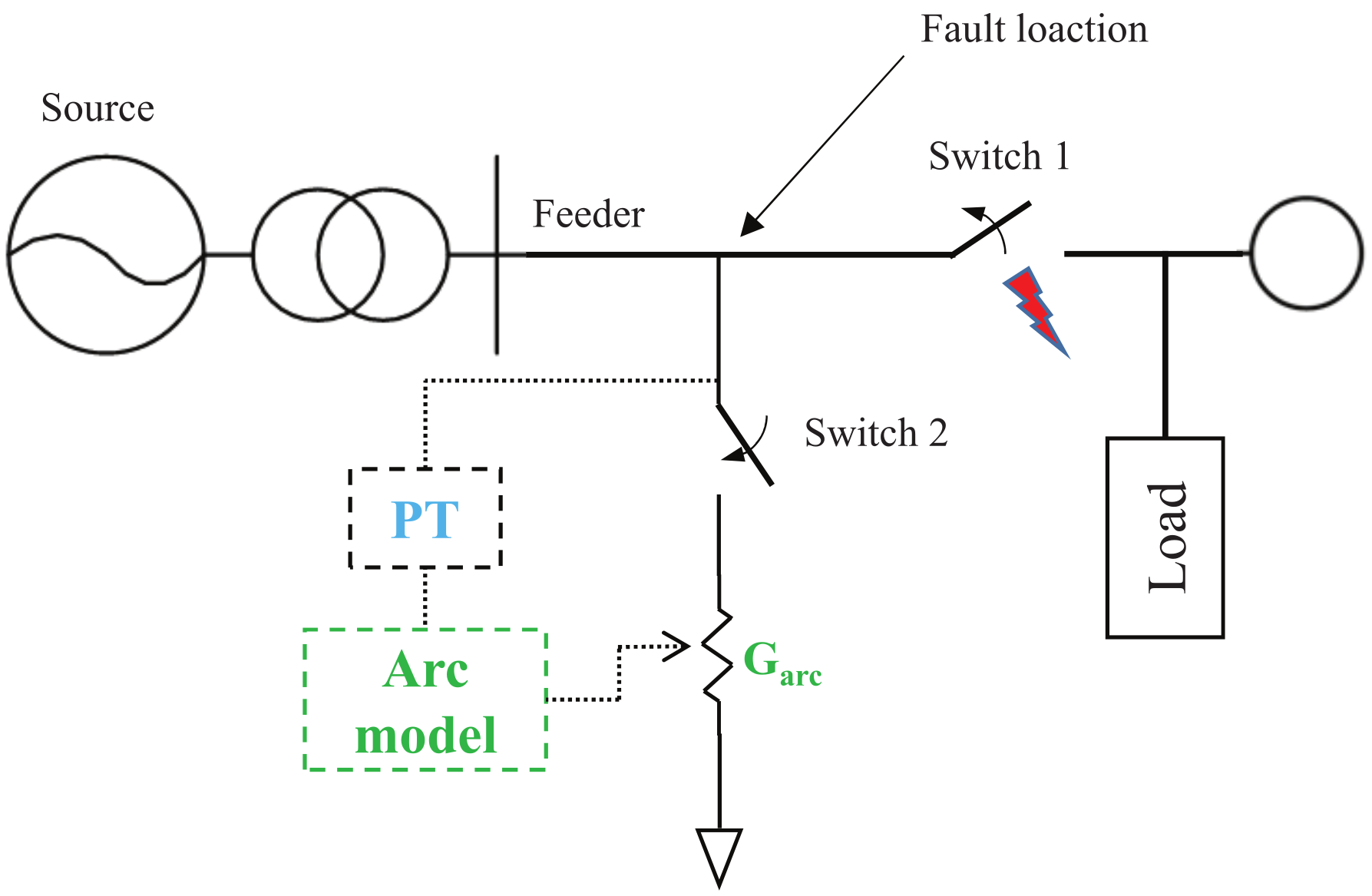
2.2. Experiment Setup

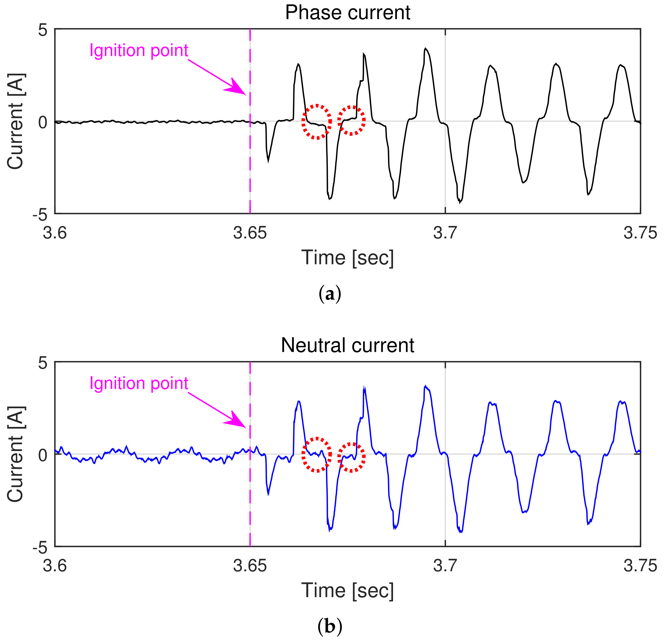
A majority of faults that occur in power distribution lines are single-phase faults. Given that an arc is created due to contact with a conductor immediately or shortly after the fault, we implemented an experiment model for a single phase fault with a contacted conductor. The power distribution network in the case of the fault with arc is depicted in Figure 1. Two time-controlled switches were added to the fault model. Switch 1 was used to simulate the fault. Switch 2 was closed to calculate arc conductance after switch 1 is opened. The distribution network operates and consists of a 3-phase 4-wire distribution feeder. Feeder remote terminal units (FRTUs) were used to measure the phase voltage and phase current at fault location to observe the wave distortion due to the arc phenomenon and was installed in the protection device and switched to verify the proposed method. FRTUs measure 1-cycle data (e.g., voltage, current magnitude, phase angle difference) through the CT and PT installed at the corresponding points. For signal processing, CPU (TMS320F2812, Texas Instrument) and A/D converters (AD7606C, Analog Device) were embedded. RS422 communication protocol was implemented for parallel data transmission. The fundamental frequency and sampling frequency correspond to 60 Hz and 20 kHz (about 333 samples per cycle), respectively. The experimental setup for arc generation is shown in Figure 2. Artificial open conductor faults were experimented on in the Gochang PTC (power testing center) of the KEPCO. The Gochang PTC had a high-voltage power distribution network, and received 22.9 kV from a substation, but no load was connected to it. For this experiment, a single branch line in the middle of the line was grounded after the open conductor, and its behaviors were analyzed.

2.3. Arc Experiment

In the arc experiment, wet gravel was used as a contacted conductor after the fault to generate arc phenomenon. The phase voltage and phase current were measured at the point of fault location and were recorded from the point after the open phase. Therefore, a fault scenario was constructed as follows:

• Step 1: Switch 1 was opened at 0 s;
• Step 2: Switch 2 was closed at 3.65 s;
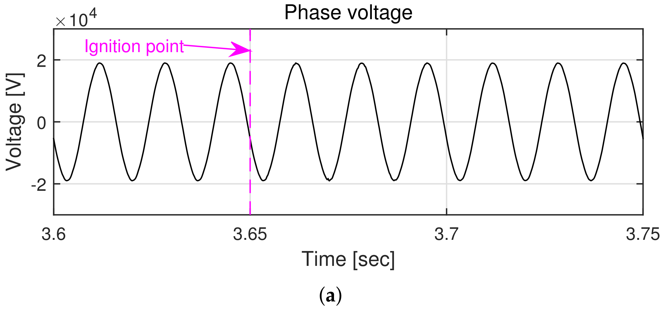
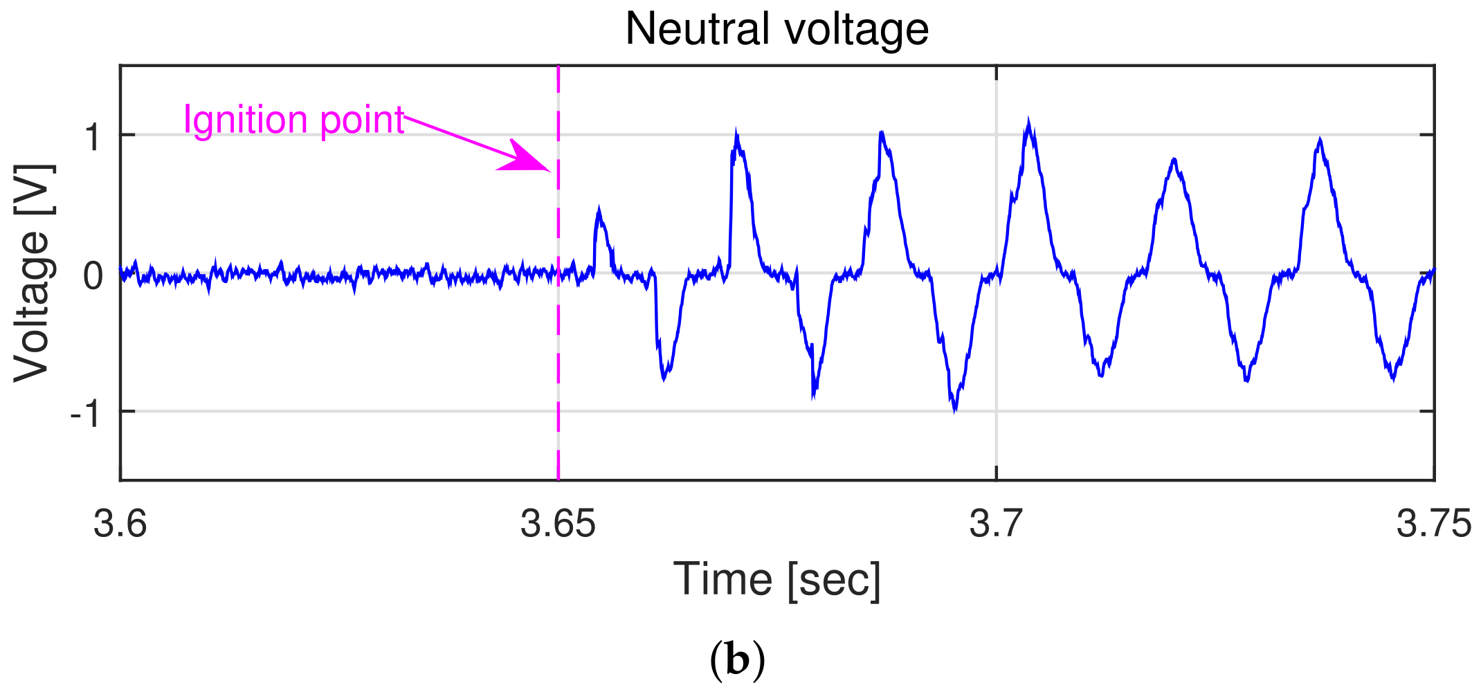
• Step 3: ignition was started after 3.65 s.

Figure 3 shows the phase voltage and neutral voltage in the fault phase and neutral line. Given that the phase voltage was supplied from the distribution system, we confirmed that there was no change in the magnitude of the phase voltage after the ignition point (at 3.65 s) because the phase voltage was continuously supplied to feeders by utility regardless of the fault. However, an unbalanced voltage was shown in Figure 3b after the ignition point in the neutral voltage due to the effect of the fault. However, since the magnitude of the neutral voltage is very small, it hardly affects the magnitude of the phase voltage.

Figure 4 shows the phase current and neutral current in fault phase and neutral line. The phase current is close to zero before the ignition point because the phase was faulted by Switch 1. Conversely, distorted currents with the same frequency as the fundamental frequency (60 Hz) were observed in phase current and neutral current. Moreover, a region with current close to zero appeared at every half cycle in the phase current and neutral current (red dotted line). This is due to the change in thermal resistance caused by faults, which is a representative nonlinear characteristic of the fault in power distribution networks. We termed this region as the shoulder region that appeared in the arc wave.

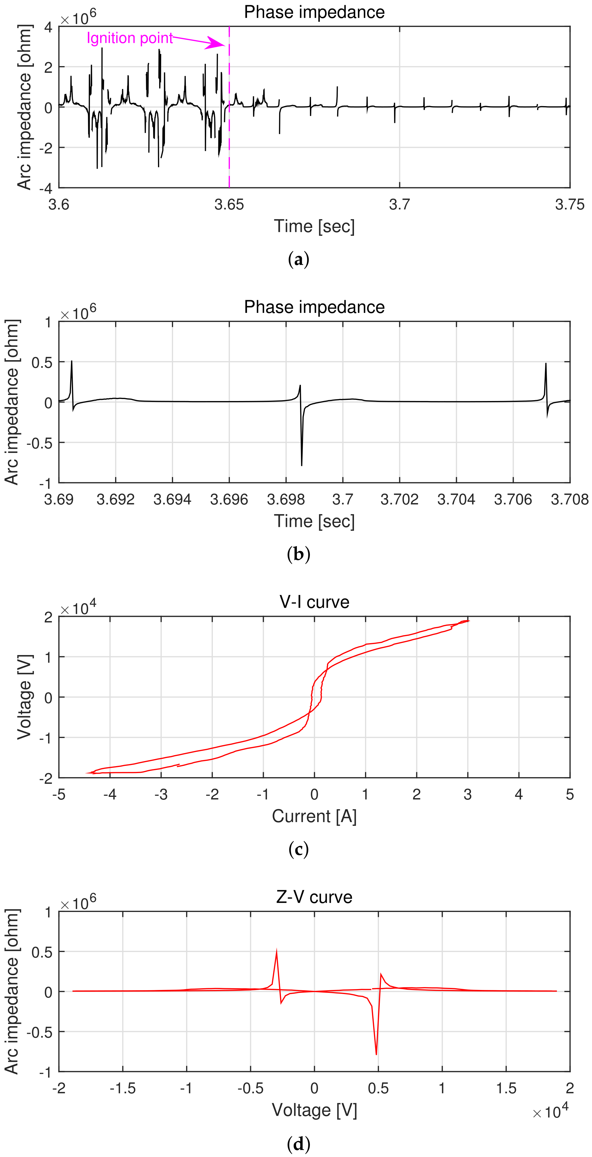
2.4. Arc Waveform Analysis

To analyze the arc waveform, we divided the experimental data into two regions. First, the data from 0 to 3.65 s was termed as the zero phase current region (i.e., infinity impedance region), and the period after 3.65 s was termed as the arc current region (i.e., arc impedance region).

Figure 5 shows arc characteristics between the phase voltage and phase current for the experiment. Before ignition point, arc impedance is almost infinite because of the distribution line insulation breakdown at fault phase. Conversely, after the fault phase line is in contact with wet gravel, phase impedance is relatively reduced, as shown in Figure 5a. This is clearly depicted in the enlarged figures at the vicinity of the zero-crossings, as shown in Figure 5b. Spikes in phase impedance appeared at points where the phase current was close to zero every half cycle of the arc current region. This revealed that the distortions in current and impedance waveforms were influenced by the arc behavior. This is clearly depicted in the V–I and Z–V curves shown in Figure 5c,d. Hysteresis nonlinearity was observed in the V–I curve due to the variation in the phase impedance. Given that the phase of the phase current can be affected by load type, the phase voltage and phase current can potentially not be in phase. Therefore, a negative phase impedance value is observed in the Z–V curve of Figure 5d.

3. Arc Modeling

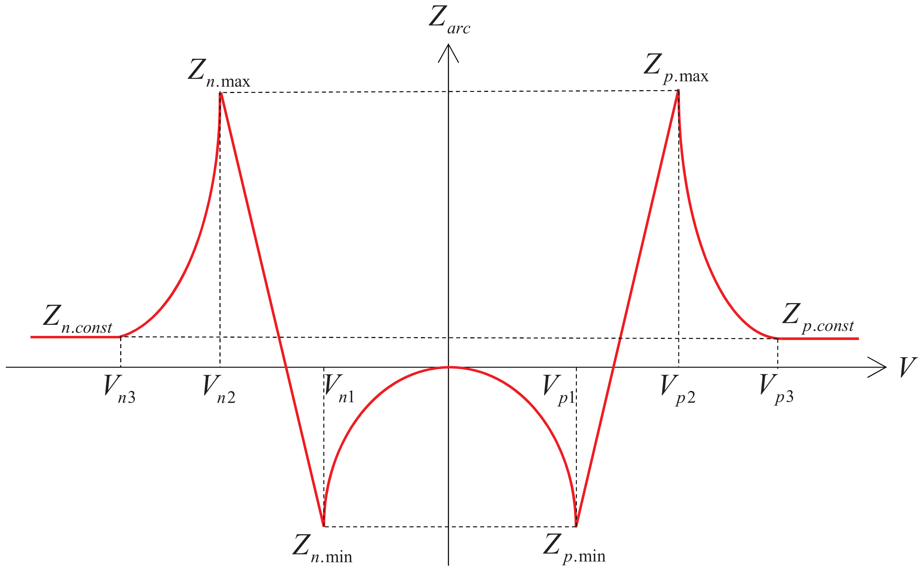
3.1. Mathematical Arc Modeling

It is difficult to accurately simulate a complete arc phenomenon due to its irregularity and reproducibility. The arc behavior changes from one half-cycle to the other half-cycle, as revealed by the experimental arc characteristics shown in Figure 5c. An arc phenomenon is composed as one cycle specific to the arc, which is characterized by unsymmetrical half cycles. Therefore, the arc parameters required for arc modeling were determined by dividing the arc region based on the amplitude of the phase voltage for each half-cycle.

Over the past few decades, many popular methods have been proposed for implementing the arc phenomenon. However, most of the previous methods use the phase current for calculating arc conductance (arc impedance) as an input of arc dynamics. Hence, it is difficult to accurately obtain the arc conductance (arc impedance) because the phase current is also affected by load fluctuation and load type. Therefore, in this study, we designed a mathematical arc model by separating two regions (viz. positive half cycle and negative half cycle) as follows:

• Positive half cycle
  After the ignition time, the arc impedance ($Z_{arc}$) can be determined by the following equations for positive phase voltage. The first and third equations are nonlinear functions and the second equation is a linear function. The last equation is defined as a constant value because there is no waveform distortion due to the arc in the region where the phase voltage exceeds $V_{th3}$.

  $$\left\{\begin{array}{c}{Z}_{p.min}exp\left(a_{p1}(V-V_{p1})\right),0\le V<V_{p1}\hfill \\ k_{p1}V+k_{p2},V_{p1}\le V<V_{p2}\hfill \\ (Z_{p.max}-Z_{p.const})exp\left(a_{p2}(V-V_{p2})\right)+Z_{p.const},V_{p2}\le V<V_{p3}\hfill \\ Z_{p.const},V\ge V_{p3}\hfill \end{array}\right.$$

  (1)

  where $k_{p1}=\frac{Z_{p.max}-Z_{p.min}}{V_{p2}-V_{p1}}$, $k_{p2}=\frac{-Z_{p.max}{V}_{p1}+Z_{p.min}{V}_{p2}}{V_{p2}-V_{p1}}$, $a_{p1}$ and $a_{p2}$ are positive integers.
• Negative half cycle
  Similar to the case of the positive half cycle, the arc impedance can be determined by the following equations for negative phase voltage:

  $$\left\{\begin{array}{c}{Z}_{n.min}exp\left(a_{n1}(-V-V_{n1})\right),V_{n1}\le V<0\hfill \\ -k_{n1}V+k_{n2},V_{n2}\le V<V_{n1}\hfill \\ (Z_{n.max}-Z_{n.const})exp\left(a_{n2}(V+V_{n2})\right)+Z_{n.const},V_{n3}\le V<V_{n2}\hfill \\ Z_{n.const},V<V_{n3}\hfill \end{array}\right.$$

  (2)

  where $k_{n1}=\frac{Z_{n.max}-Z_{n.min}}{V_{n2}-V_{n1}}$, $k_{n2}=\frac{-Z_{n.max}{V}_{n1}+Z_{n.min}{V}_{n2}}{V_{n2}-V_{n1}}$, $a_{n1}$ and $a_{n2}$ are positive integers.

Figure 6 shows the proposed arc model, which calculates the arc impedance by using the phase voltage as the input. Since arc impedance depends on the magnitude of the phase voltage, the proposed arc model consists of the nonlinear arc impedance region $V_{n3}$, $V_{n2}$], [$V_{n1}$, $V_{p1}$], [$V_{p2}$, $V_{p3}$]), linear impedance region ([ $V_{n2}$, $V_{n1}$], [$V_{p1}$, $V_{p2}$]), constant arc impedance region ([ $-\infty$, $V_{n3}$], [$V_{p3}$, ∞]).

The corresponding simulated arc characteristics are illustrated in the comparison shown in Figure 7. We can observe that two V–I curves are similar and have small relative error between the experimental model and simulation model, even if the V–I curve has nonlinearity and asymmetry. The arc parameters are determined such that they match the results of V–I and Z–V curves in the arc experiment. These comparisons verify the accuracy of the arc model. As shown in the comparison results, the simulated arc model is similar to the experimental arc model. The arc parameters used in arc modeling are listed in

Table 1. Arc parameters used in the simulations. (Unit: impedance: [$\Omega$], voltage: [V]).

Arc Parameter	Designed Value	Arc Parameter	Designed Value
$Z_{p.max}$	212,900	$V_{p1}$	4842
$Z_{p.min}$	−693,300	$V_{p2}$	5197
$Z_{n.max}$	685,500	$V_{p3}$	5500
$Z_{n.min}$	−143,000	$V_{n1}$	−2619
$Z_{p.const}$	7000	$V_{n2}$	−2963
$Z_{n.const}$	5000	$V_{n3}$	−6500
$a_{p1}$	0.003	$a_{n1}$	0.001
$a_{p2}$	0.002	$a_{n2}$	0.01

.

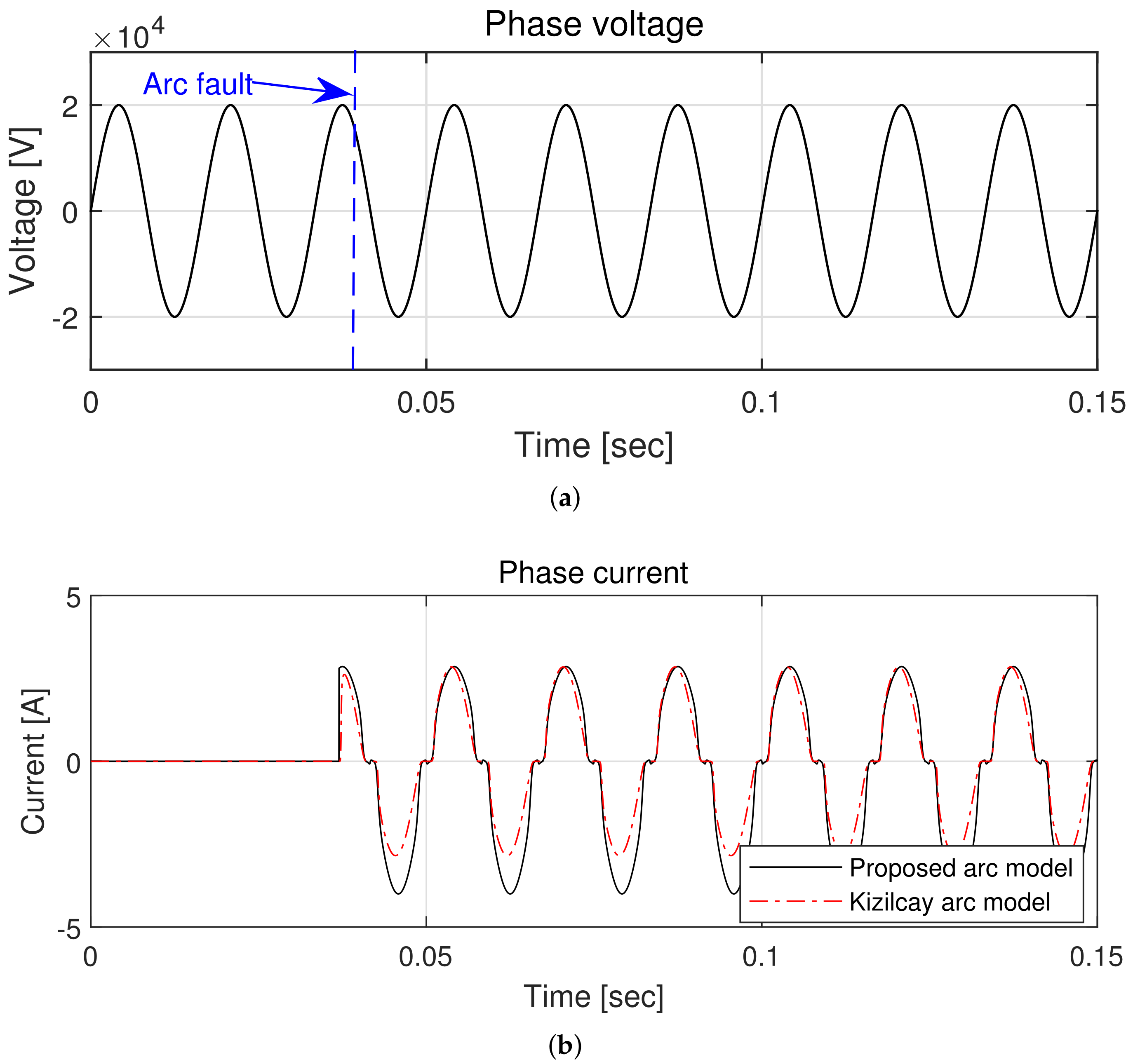
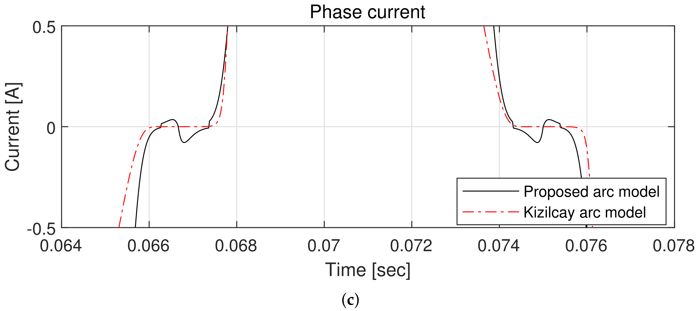
3.2. Model Verification

In this subsection, we discuss the simulation results to verify the success of arc modeling. To show the effectiveness of the proposed arc model, simulations were performed in a single-phase distribution feeder with conditions similar to those of the experiment using Matlab/Simulink. The description for the simulation is shown in Figure 1. To implement the fault, two switches were used. Switch 1 was opened for the open phase fault when the simulation started. Switch 2 was closed to implement the fault with arc at the arc fault time (0.037 [s]). The sampling frequency and control frequency (e.g., control input generation period at each sample) were 50 [kHz]. The arc equations were solved using the Runge–Kutta 4th order solver. The supplying phase voltage and fundamental frequency were set to 20 kV and 60 Hz, respectively, which were identical to those in the experiment.

The Kizilcay’s arc model [20] was used as a comparison method as follows:

$$\begin{array}{c}\hfill \begin{array}{cc}\hfill \frac{dg}{dt}& =\frac{1}{\tau }(\frac{\left|i\right|}{V_{arc}}-g)\hfill \end{array}\end{array}$$

(3)

where $\tau =A{e}^{Bg}$. In addition, g is the time varying arc conductance, $\left|i\right|$ is the absolute value of the arc current, $V_{arc}$ is a constant arc voltage, $\tau$ is the arc time constant. To implement Kizilcay’s arc model, the parameters, A, B, and $V_{arc}$, are set to $6.6\times {10}^{-5}$, $41.97$, and 4520, respectively.

Figure 8 shows the phase voltage and phase current by using the proposed and Kizilcay’s arc model in the simulations. The phase voltages are the same in both method because phase voltages are injected from utility. Before the ignition, the phase impedance should be almost infinite in the remaining load path because there is no arc model path. Therefore, the phase current became almost zero when the phase was opened. Then, fault currents were generated after the arc fault time (0.037 [s]) in both methods. In Figure 8c, we observe that the proposed arc model had the shoulder phenomenon with nonlinearity around zero current at every half cycle because of the arc generated by (1) and (2). This nonlinearity is generated by time-varying impedances where the arc impedance is not constant. There is a buildup phenomenon with arc fault characteristics. However, because this phenomenon is not well observed due to the fast time constant in the arc experiment, it was not considered in the arc modeling procedure. Based on these results, the arc model appeared to have been accurately represented.

4. Fault Detection and Power System Simulations

In this section, we discuss the fault detection algorithm and its simulation results. First, the balanced three-phase currents are defined as follows:

$$\begin{array}{c}\hfill \begin{array}{cc}\hfill I_a& =I_{m}sin\left(\omega t\right)\hfill \\ \hfill I_b& =I_{m}sin(\omega t+\frac{2}{3}\pi )\hfill \\ \hfill I_c& =I_{m}sin(\omega t-\frac{2}{3}\pi )\hfill \end{array}\end{array}$$

(4)

where $I_m$ denotes the amplitude of phase currents, $\omega$ denotes the fundamental frequency in the distribution network and $\pi$ corresponds to 180 degrees.

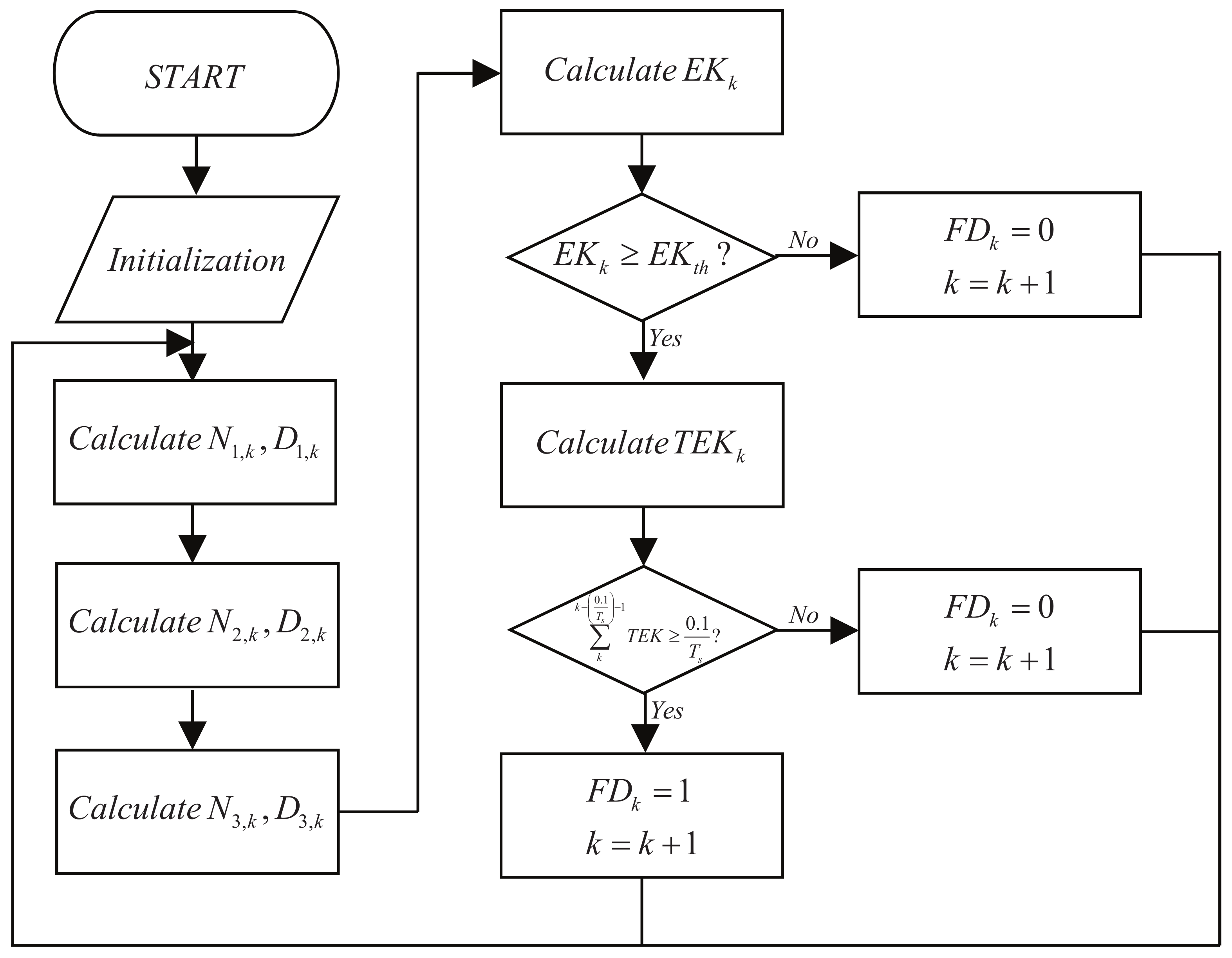
4.1. Fault Detection Logic Using Kurtosis Detection

Spectral kurtosis is a useful tool, which is capable of detecting non ideal components in a signal. Given these advantages, various kurtosis detection methods, such as tooth crack detection of wind turbines [21], stable operation of power systems [22] and electric motor bearing fault detection [23] have been applied in industrial applications.

As described in Section 4, when the fault with arc exists, the phase current contains shoulder phenomenon in the faulted line. This shoulder phenomenon results in a nearly zero current region and a relatively sharper peak of the distribution of the phase current signal’s amplitude compared with the Gaussian distribution, leading to an increase in the kurtosis index. On the other hand, when the fault does not exist, its distribution is closed to the Gaussian distribution, which ideally has a kurtosis index of 3. Suppose that the fault with arc has occurred in phase A, let us define the discrete time signal of the phase current as follows:

$$\begin{array}{c}\hfill \begin{array}{cc}\hfill I_a\left[k\right]& =I_{m}sin\left(\omega T_{s}k\right)\hfill \end{array}\end{array}$$

(5)

where $T_s$ and k are the sampling interval and sampling index, respectively. For a signal $I_a\left[k\right]$, the excess kurtosis index is defined as follows:

$$\begin{array}{c}\hfill \begin{array}{cc}\hfill EK\left[I_a\right]& =\frac{\frac{1}{N}\left[{\displaystyle \sum _{i=k}^{k+N-1}}{(I_a\left[k\right]-\overline{I_a})}^4\right]}{{\left(\frac{1}{N}\left[{\displaystyle \sum _{i=k}^{k+N-1}}{(I_a\left[k\right]-\overline{I_a})}^2\right]\right)}^2}-K_{Gaussian}\hfill \end{array}\end{array}$$

(6)

where N and $\overline{I_a}$ denote the number of $I_a\left[k\right]$ and the mean of $I_a\left[k\right]$ during the N period, respectively. Additionally, $K_{Gaussian}$ denotes the kurtosis index of the Gaussian distribution. The proposed fault detection logic can be presented in Algorithm 1. Description of the variables used in Algorithm 1 are as follows:

• k: sampling index of digital processor;
• $N_{1,k}$: numerator coefficient at the k-th sampling index;
• $D_{1,k}$: denominator coefficient at the k-th sampling index;
• $N_{2,k}$: numerator coefficient for the N-th period;
• $D_{2,k}$: denominator coefficient for the N-th period;
• $N_{3,k}$: numerator average coefficient for the N-th period;
• $D_{3,k}$: denominator average coefficient for the N-th period;
• $E{K}_k$: excess kurtosis value at the k-th sampling index;
• $E{K}_{th}$: excess kurtosis threshold value;
• $CE{K}_k$: arbitrary excess kurtosis value at the k-th sampling index;
• $TE{K}_k$: total excess kurtosis value at the k-th sampling index;
• $F{D}_k$: fault detector value at the k-th sampling index.

A flowchart of Algorithm 1 is shown in Figure 9.

Algorithm 1 The pseudo-code describing the proposed fault detection method is presented

1:  Let $N\leftarrow floor(\omega /\left(2\pi T_s\right))$ 2:                     ▹N: Sampled data number of moving window 3:  $\overline{I_a}\leftarrow 0$, $k\leftarrow 1$, $TEK\leftarrow 0$, $CEK\leftarrow 0$, $K_{Gaussian}\leftarrow 1.5$      ▹ Initialization 4:  function Fault Detector($I_a,N$) 5:   while $k+N-1\le L$do                     ▹L: $maxk$ 6:    for $i=k$ to $k+N-1$ do 7:     $N_{1,k}\leftarrow {(I_a\left[k\right]-\overline{I_a})}^4$ 8:     $D_{1,k}\leftarrow {(I_a\left[k\right]-\overline{I_a})}^2$ 9:     $N_{2,k}\leftarrow {\displaystyle \sum _{i=k}^{k+N-1}}{N}_{1,k}$ 10:     $D_{2,k}\leftarrow {\displaystyle \sum _{i=k}^{k+N-1}}{D}_{1,k}$ 11:     $N_{3,k}\leftarrow \frac{N_{2,k}}{N}$ 12:     $D_{3,k}\leftarrow {\left(\frac{D_{2,k}}{N}\right)}^2$ 13:     $E{K}_k\leftarrow \frac{N_{3,k}}{D_{3,k}}$ 14:     if $E{K}_k\ge E{K}_{th}$ then 15:      $CE{K}_k\leftarrow 1$ 16:      $TE{K}_k={\displaystyle \sum _{i=k-(1/\left(10T_s\right)-1)}^k}CE{K}_k$ 17:      if ${\sum }_{TE{K}_{k-(1/\left(10T_s\right)-1)}}^{TE{K}_k}\ge 1/\left(10T_s\right)$ then 18:       $F{D}_k\leftarrow 1$ 19:      else 20:       $F{D}_k\leftarrow 0$ 21:      end if 22:     else 23:      $CE{K}_k\leftarrow 0$ 24:      $TE{K}_k\leftarrow 0$ 25:      $F{D}_k\leftarrow 0$ 26:     end if 27:     $k=k+1$                      ▹i: index update 28:    end for 29:   end while 30:  end function

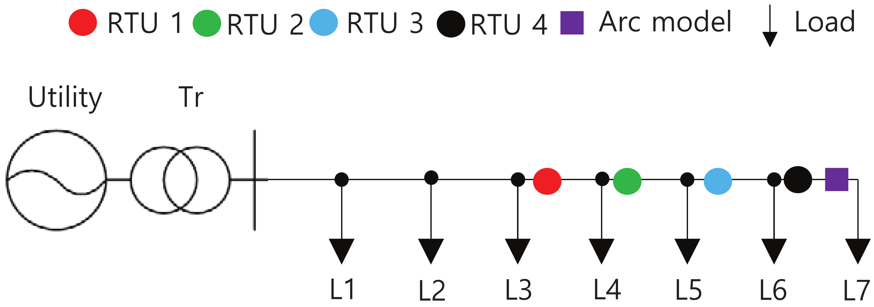
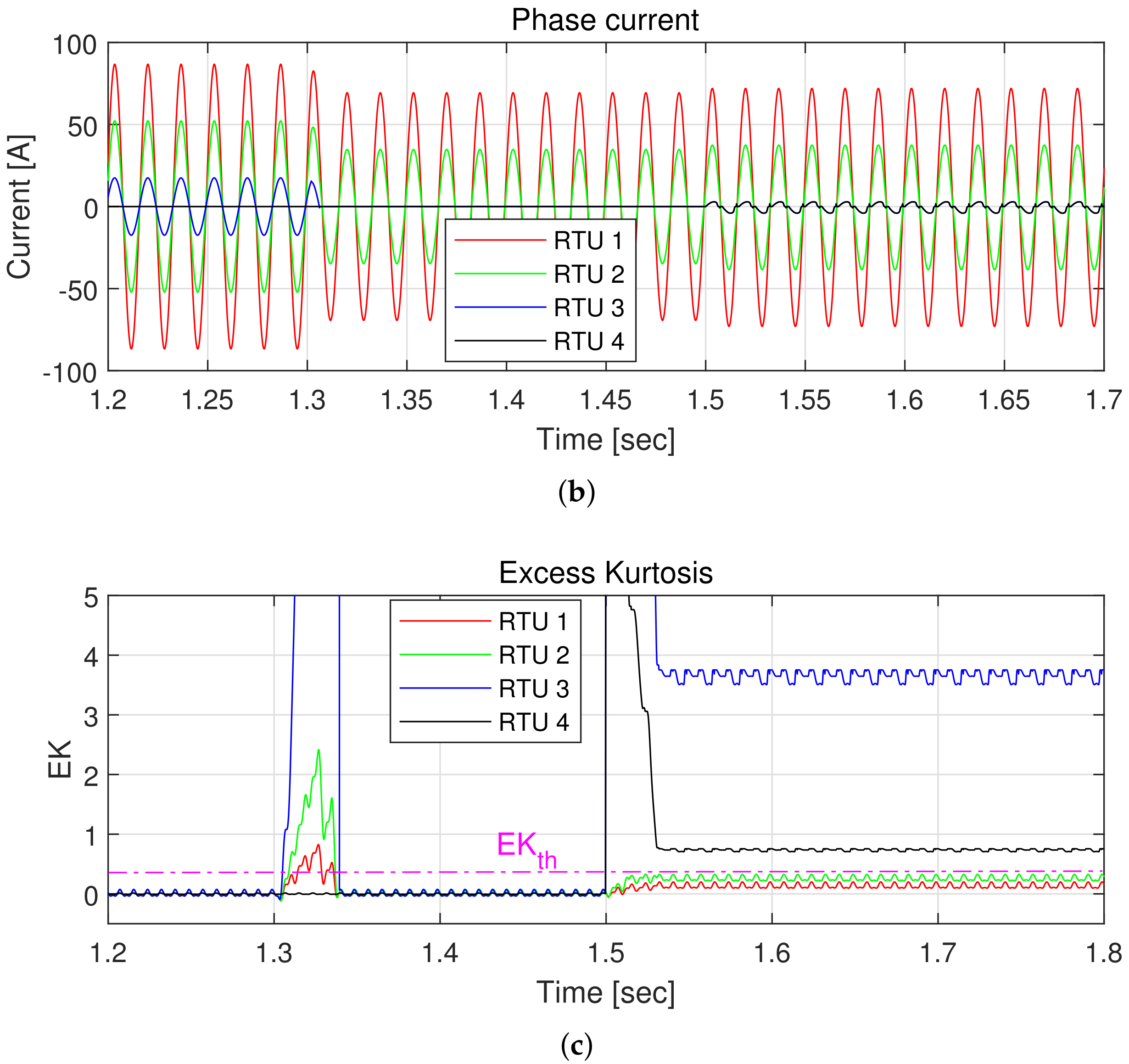
4.2. Power System Simulation

The simulations were conducted to evaluate the fault detection method developed in the study. The test system is shown in Figure 10. It models a 22.9 kV distribution feeder from the general test system of Korean Electric Power Corporation. The feeder included a 154–22.9 kV transformer that connected the utility and feeder. The fundamental frequency and sampling frequency corresponded to 60 Hz and 6 kHz, respectively. Therefore, N is set to 100. Subsequently, $K_{Gaussian}$ was defined as 1.5 to calculate excess kurtosis. Furthermore, $E{K}_{th}$ was set to 0.4 for fault detection. Four RTUs were used to obtain phase currents and kurtosis indexes at different locations. In general, electric arcs were generated after a certain amount of time elapsed after the phase opening. Thus, in the simulation, a fault scenario was constructed in which the fault occurred 1 s after the simulation commenced and then load switching was produced for $L6$ of the system load at 1.3 s, finally the fault arc occurred after 1.5 s.

Figure 11 shows phase currents and excess kurtosis indices. As shown in Figure 11a, the magnitude of the phase current decreases as the distance from an overhead feeder of power system increases. We observe that the phase current at RTU 4 is nearly zero after 1 s, as shown in Figure 11b because of the infinite load impedance value when the fault occurs immediately behind RTU 4 as shown in Figure 10. Conversely, although the phase currents were reduced in other RTUs, it was confirmed that the phase currents did not correspond to 0. This is due to the fact that the load impedances at each RTU exhibited finite values although the load impedances changed. After 1.5 s, the shoulder phenomenon, which is a typical fault with arc, was observed in RTU 4. After 1.3 s, the phase current at RTU 3 is nearly zero because the load switching was produced for $L6$. Figure 11c shows excess kurtosis indices. After 1.5 s, the change in excess kurtosis index was observed when the arc occurred, and it was observed that the distances from the fault point to the RTU were inversely proportional to the values of the excess kurtosis index. Since the load switching was produced, variation of EK value was briefly observed during 0.05 s after 1.3 s. Additionally, EK was set to 0.4 for fault detection as a threshold value of excess kurtosis index.

Figure 12 shows fault detection performance at each RTU. Faults were detected in RTU 3 and RTU 4, which were relatively close to the fault location. However, they were not detected in RTU 1 and RTU 2. Even if it can be seen that the EK is not zero by an effect on the load switching from 1.3 s to 1.35 s, ED values calculated from all RTUs are continuously zero before the arc ignition due to inconsistency of the EK value.

5. Conclusions

In this paper, we developed a mathematical arc model of fault in power distribution networks. The arc experiment was performed to ascertain arc fault characteristics and thereby aid in arc modeling. A new arc model was developed using only phase voltage as input, and arc parameters were determined based on the experiment results. An arc detection method based on kurtosis detector was developed to detect the arc fault. Furthermore, power system simulations were performed under various fault scenarios such as load impedance change to confirm the effectiveness of the proposed arc detection algorithm.

One possible future work would be to consider other faults such as fault location detection, various closed-circuit high impedance faults, multi-phase faults and transmission line faults.

References

1. Elkalashy, N.I.; Lehtonen, M.; Darwish, H.A.; Izzularab, M.A.; Taalab, A.I. Modeling and experimental verification of high impedance arcing fault in medium voltage networks. IEEE Trans. Dielectr. Electr. Insul. 2007, 14, 375–383. [Google Scholar] [CrossRef]
2. Iurinic, L.U.; Herrera-Orozco, A.R.; Ferraz, R.G.; Bretas, A.S. Distribution systems high-impedance fault location: A parameter estimation approach. IEEE Trans. Power Deliv. 2016, 31, 1806–1814. [Google Scholar] [CrossRef]
3. Cui, Q.; Weng, Y. Enhance high impedance fault detection and location accuracy via μ-PMUs. IEEE Trans. Smart Grid 2020, 11, 797–809. [Google Scholar] [CrossRef]
4. Friedemann, D.F.; Motter, D.; Oliveira, R.A. Stator-ground fault location method based on third-harmonic measures in high-impedance grounded generators. IEEE Trans. Power Electron. 2021, 36, 794–802. [Google Scholar] [CrossRef]
5. Chakraborty, S.; Das, S. Application of smart meters in high impedance fault detection on distribution Systems. IEEE Trans. Smart Grid 2019, 10, 3465–3473. [Google Scholar] [CrossRef]
6. Torres, V.; Guardado, J.L.; Ruiz, H.F.; Maximov, S. Modelling and detection of high impedance faults. Int J Electr. Power Energy Syst. 2014, 61, 163–172. [Google Scholar] [CrossRef]
7. Lopes, G.N.; Menezes, T.S.; Santos, G.G.; Trondoli, L.H.P.C.; Vieira, J.C.M. High impedance fault detection based on harmonic energy variation via S-transform. Int. J. Electr. Power Energy Syst. 2022, 136, 107681. [Google Scholar] [CrossRef]
8. Wang, B.; Cui, X. Nonlinear modeling analysis and arc high-impedance faults detection in active distribution networks with neutral grounding via petersen coil. IEEE Trans. Smart Grid 2022. [Google Scholar] [CrossRef]
9. Gajula, K.; Herrera, L. Detection and localization of series arc faults in DC microgrids using Kalman filter. IEEE J. Emerg. Sel. Top. Power Electron. 2021, 9, 2589–2596. [Google Scholar] [CrossRef]
10. Lee, C.-K.; Chang, S.J. A Method of fault localization within the blind spot using the hybridization between TDR and wavelet transform. IEEE Sens. J. 2021, 21, 5102–5110. [Google Scholar] [CrossRef]
11. Sedighi, A.-R.; Haghifam, M.-R.; Malik, O.P.; Ghassemian, M.-H. High impedance fault detection based on wavelet transform and statistical pattern recognition. IEEE Trans. Power Deliv. 2005, 20, 2414–2421. [Google Scholar] [CrossRef]
12. Lima, E.M.; Junqueira, C.M.; Brito, N.S.; Souza, B.A.; Coelho, R.A.; Medeiros, H.G. High impedance fault detection method based on the short-time Fourier transform. IET Gener. Transm. Distrib. 2018, 12, 2577–2584. [Google Scholar] [CrossRef]
13. Eskandari, A.; Milimonfared, J.; Aghaei, M. Fault detection and classification for photovoltaic systems based on hierarchical classification and machine learning technique. IEEE Trans. Ind. Electron. 2021, 58, 12750–12759. [Google Scholar] [CrossRef]
14. Rai, K.; Hojatpanah, F.; Ajaei, F.B.; Grolinger, K. Deep learning for high-impedance fault detection: Convolutional autoencoders. Energies 2021, 14, 3623. [Google Scholar] [CrossRef]
15. Cui, Q.; El-Arroudi, K.; Weng, Y. A feature selection method for high impedance fault detection. IEEE Trans. Power Deliv. 2019, 34, 1203–1215. [Google Scholar] [CrossRef] [Green Version]
16. Ohtaka, T.; Kertesz, V.; Smeets, R. Novel black-box arc model validated by high-voltage circuit breaker testing. IEEE Trans. Power Deliv. 2018, 33, 1835–1844. [Google Scholar] [CrossRef]
17. Khakpour, A.; Franke, S.; Gortschakow, S.; Uhrlandt, D.; Methling, R.; Weltmann, K.-D. An improved arc model based on the arc diameter. IEEE Trans. Power Deliv. 2016, 31, 1335–1341. [Google Scholar] [CrossRef]
18. Guo, M.-F.; Cai, W.-Q.; Zheng, Z.-Y.; Hui, W. Fault phase selection method based on single-phase flexible arc suppression device for asymmetric distribution networks. IEEE Trans. Power Deliv. 2022. [Google Scholar] [CrossRef]
19. Parise, G.; Martirano, L.; Laurini, M. Simplified arc-fault model: The reduction factor of the arc current. IEEE Trans. Ind. Appl. 2013, 49, 1703–1710. [Google Scholar] [CrossRef]
20. Kizilcay, M.; Pniok, T. Digital simulation of fault arcs in power systems. Eur. Trans. Electr. Power 1991, 1, 55–60. [Google Scholar] [CrossRef]
21. Barszcz, T.; Randall, R.B. Application of spectral kurtosis for detection of a tooth crack in the planetary gear of a wind turbine. Mech. Syst. Signal Proc. 2009, 23, 1352–1365. [Google Scholar] [CrossRef]
22. Wu, J.; Qiu, H.; Xu, J.; Zhou, F.; Dai, K.; Yang, C.; Lv, D. Quantifying harmonic responsibilities based on kurtosis detection principle of amplitude fluctuations. IEEE Access 2018, 6, 64292–64300. [Google Scholar] [CrossRef]
23. Tian, J.; Morillo, C.; Azarian, M.H.; Pecht, M. Motor bearing fault detection using spectral kurtosis-based feature extraction coupled with K-nearest neighbor distance analysis. IEEE Trans. Ind. Electron. 2016, 63, 1793–1803. [Google Scholar] [CrossRef]
Figure 1. Description for power distribution network in case of fault with arc [6].
Applsci 12 02777 g001
Figure 2. Experimental setup for arc generation. (a) Experiment environment. (b) Arc generation.
Applsci 12 02777 g002aApplsci 12 02777 g002b
Figure 3. Phase voltage and neutral voltage in experiments. (a) Phase voltage. (b) Neutral voltage.
Applsci 12 02777 g003aApplsci 12 02777 g003b
Figure 4. Phase current and neutral current in experiments. (a) Phase current. (b) Neutral current.
Applsci 12 02777 g004
Figure 5. Experimental arc characteristics. (a) Phase impedance. (b) Phase impedance (1 cycle). (c) Voltage-current curve (1 cycle). (d) Impedance-voltage curve (1 cycle).
Applsci 12 02777 g005
Figure 6. Proposed arc model (proposed Z–V curve).
Applsci 12 02777 g006
Figure 7. Comparison of simulated and experimental arc characteristics. (a) Voltage-current curves for both simulated and experimental arc models. (b) Impedance-voltage curves for both simulated and experimental arc models.
Applsci 12 02777 g007
Figure 8. Phase voltage and phase current in simulations. (a) Phase voltage. (b) Phase current. (c) Phase current (zoomed in x- and y-axis).
Applsci 12 02777 g008aApplsci 12 02777 g008b
Figure 9. Flowchart of the proposed fault detection algorithm.
Applsci 12 02777 g009
Figure 10. Test system.
Applsci 12 02777 g010
Figure 11. Phase currents and excess kurtosis indices. (a) Phase current. (b) Phase current (zoomed in x-axis). (c) Excess kurtosis.
Applsci 12 02777 g011aApplsci 12 02777 g011b
Figure 12. Fault detection performance at each RTU. (a) RTU1; (b) RTU2; (c) RTU3; (d) RTU4.
Applsci 12 02777 g012aApplsci 12 02777 g012b