Investigation on Aerodynamic Noise Characteristics of Coaxial Rotor in Hover

Abstract

A numerical method based on Reynolds Averaged Navier–Stokes (RANS) equations and a high-efficiency trim model is developed to simulate the aerodynamics of a coaxial rotor. Farassat 1A equations are used for the prediction of thickness and loading noise. Hover cases of different thrust coefficients with torque balance are conducted. The sound pressure history of different observation points positioned below the rotor disk plane is analyzed. Results indicate that the special noise characteristics of the coaxial rotor are mainly caused by the noise superposition of the twin rotors and the unsteady loads of aerodynamic interaction. A new kind of impulsive loading noise is induced by the blade-meeting interaction. In contract to the single rotor, the loading noise of a coaxial rotor has a much larger sound pressure level in the high-frequency band. The loading noise is obviously enhanced around the blade-meeting azimuths. The maximum noise of the coaxial rotor is located immediately below the rotor disk center, while for the single rotor, it is the minimum location.

1. Introduction

Nowadays, high-speed capability is an important requirement in the design of helicopters. Several novel configurations have been put forward to meet this requirement. Compared with the conventional configuration of a single rotor, a rigid coaxial rotor compound helicopter has substantial advantages in aerodynamic performance [1]. Sikorsky Aircraft developed the X2 Technology^TM Demonstrator aircraft based on the advancing blade concept (ABC) [2]. Its cruise speed is considerably higher than a conventional single-rotor helicopter [3]. However, a rigid coaxial rotor meets severe aerodynamic interaction, as a small rotor space is usually adopted to reduce the drag in forward flight. Correspondingly, this will cause complex interaction loads and special aerodynamic noise characteristics.

Current research studies of coaxial rotors are mostly focused on the aerodynamic interaction problems [4,5]. These provide important references for the acoustic analysis. However, studies about the aerodynamic noise of coaxial rotors are still limited. Ffowcs Williams–Hawkings (FW-H) equations have been widely used in rotor aeroacoustics research [6]. In 2006, Wachspress et al. [7] established the calculation method for the linear noise of a coaxial rotor based on an acoustic prediction program, WOPWOP, and studied the influence of configuration parameters on aerodynamic noise. The vortex line method was used to calculate the blade surface load. Kim et al. [8,9] built an acoustics prediction model based on the vorticity transport model (VTM), and investigated the blade–vortex interaction noise of a coaxial rotor in inclined descent. The wake characteristics of a coaxial rotor can be computed with reasonable accuracy by vortex methods. However, vortex methods are usually dependent on empirical formulas and the detailed unsteady interaction loads cannot be simulated well [10,11]. By comparison, the CFD method has many more advantages in the flow field simulation of a coaxial rotor, which can simulate the actual blade motions and detailed flow field of interaction.

In 2016, Walsh et al. [12] analyzed the acoustics of a coaxial rotor based on the Rotorcraft Comprehensive Analysis System (RCAS), and found a new kind of impulsive sound pressure pulse at high-speed forward flight. Zhu and Wang et al. [13,14] analyzed the noise characteristics of a coaxial rotor in hover based on Farassat 1A equations and Reynolds Averaged Navier–Stokes (RANS) equations. However, the detailed causes of noise characteristics had not been studied. In recent years, Jia et al. [15,16,17] used the CFD/CSD loose coupling method and PSU-WOPWOP program and conducted a series of studies of lift-offset coaxial rotor acoustics. The impulsive loading noise was found to be caused by “blade-crossover” interaction events. Based on the previous research, there are two main differences in coaxial rotor noise in hover, compared with a single rotor. At one aspect, the noise is formed by the superposition of two noise sources, contra-rotating rotors. Meanwhile, there are special interaction phenomena for a rigid coaxial rotor, which would cause new loading noise characteristics.

At hover state, there is no aerodynamic interaction for a single rotor, meaning that the rotor load is quasi-steady. Thus, interactions of the coaxial rotor can be clearly explained through comparison. Meanwhile, hovering is the typical interaction state of a coaxial rotor, especially for the blade-meeting interaction. In forward flight, there are complex interactions, which makes it difficult to reveal the formation mechanism of noise. Thus, for the hover state, it is necessary to carry out a further analysis on the aerodynamic noise of a coaxial rotor, referring to the mechanism of interaction. This paper is further research based on the previous research [18,19]. The previous CFD solver based on the RANS solver and moving overset mesh are adopted for flow field simulation, which provides sound source information. The acoustic method is developed based on Farassat 1A equations [20]. Meanwhile, a high-efficiency delta trim method [18] for a coaxial rotor is used to achieve torque balance. The rotating noise, including the thickness and loading noise, of a model rotor in single and coaxial configurations in hover is investigated. Through the analysis, the characteristics and generation mechanism of coaxial rotor noise are illustrated.

2. Methodology

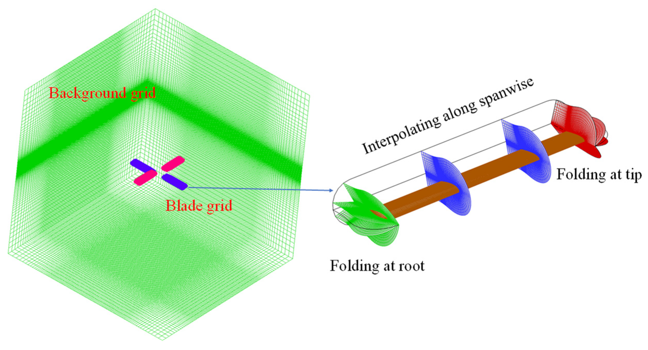
2.1. CFD Method and Trim Model

The CFD solver used in this paper was developed in Refs. [18,19]. Navier–Stokes equations [21] in an inertial Cartesian coordinate system are employed to simulate the rotor flow field, which can be written as

$$\frac{\partial }{\partial t}{{\displaystyle \iiint }}_{\partial V}WdV+{{\displaystyle ∯}}_{\partial S}\left(F_c-F_v\right)·ndS=0$$

(1)

where W represents the vector of conservative variables, F_c is the vector of the convective flux, and F_v is viscous flux.

The governing equations are spatially discretized by the finite volume method. The Roe scheme is employed to compute the inviscid flux terms. A three-order monotone upwind-centered scheme for conservation laws (MUSCL) [22] is applied to reconstruct variables in a control volume. The viscous flux terms are discretized by adopting a second-order central difference scheme. The one-equation Spalart–Allmaras turbulence model [23] is used to simulate the turbulent viscosity. The dual time-stepping approach is employed for temporal discretization. The implicit lower-upper symmetric Gauss–Seidel (LUSGS) [24] scheme is used for the calculation of the pseudo-timestep. In the following computations, the sub-iteration of the pseudo-timestep is set as 8 for the single rotor, and for the coaxial rotor, it is 20 to recover higher time accuracy. The physical timestep is set as 1440 in one resolution, meaning that each time interval corresponds to 0.25° azimuth.

A moving overset mesh system is employed to simulate the contra-rotating of rotors. The mesh system consists of the Cartesian background mesh and the body-fitted blade mesh with C-O type. The mesh of the blade tip is refined spanwise. The background mesh in the region where the rotors lie is also refined to capture the details of rotor wake. The mesh system of blade and background is shown in Figure 1.

The research is conducted with a two-bladed model rotor. The blades use NACA0012 airfoil sections with no twist. The parameters are given in

Table 1. Parameters of the model coaxial rotor in this paper.

Parameter	Values
Rotor radius	2.0 m
Rotor cutout	0.212 R
Chord	0.22 m
Number of blades	2 + 2
Twist	None
Blade tip Mach number	0.5878
Rotor vertical distance	0.15 R

. Each blade mesh has 221 × 78 × 102 points in the streamwise, normal, and spanwise directions, respectively. The background mesh has 235 × 196 × 235 points in the x, y, and z directions. The background mesh is refined in the region of rotor wake. The refined mesh spacing of the blade tip and background near the rotor tip is approximately 0.05 c for both, which is set according to the previous calculation experience of coaxial rotors. The total number of mesh points is approximately 17.85 million.

In order to obtain a specific value of thrust and achieve torque balance, an efficient CFD trim model [18] for a coaxial rotor is adopted. This trim model was developed from the “delta method”, which has been applied in the single rotor [25,26]. In the model, the blade element moment theory (BEMT) and CFD solver of the coaxial rotor are coupled with each other, which can significantly improve the efficiency and ensure the accuracy. A detailed introduction to the trim model can be found in Refs. [18,19]. The trimmed collective pitches for various rotor thrusts in hover are given in

Table 2. Trimmed collective pitches for the coaxial rotor.

Case	CT	θ0U (°)	θ0L (°)
A0	0.0	0	0
A1	0.004	6.03	6.42
A2	0.010	9.92	10.21

.

2.2. Acoustic Prediction Model

The acoustic prediction model for a coaxial rotor is built based on that for a single rotor [27,28], where Farassat 1A formulations [20] are adopted. For an impermeable data surface, such as the blade surface, the acoustic pressure time history is given by

$$p^{\prime }\left(x,t\right)=p_T^{\prime }\left(x,t\right)+p_L^{\prime }\left(x,t\right)$$

(2)

$$4\pi p_T^{\prime }\left(x,t\right)={{\displaystyle \int }}_{f=0}{\left[\frac{{\rho }_0{\dot{v}}_n}{r{(1-M_r)}^2}+\frac{{\rho }_0{v}_n{\widehat{r}}_i{\dot{M}}_i}{r{(1-M_r)}^3}\right]}_{ret}dS+{{\displaystyle \int }}_{f=0}{\left[\frac{{\rho }_0{c}_0{v}_n\left(M_r-M^2\right)}{r^2{(1-M_r)}^3}\right]}_{ret}dS$$

(3)

$$4\pi p_L^{\prime }\left(x,t\right)=\frac{1}{c_0}{{\displaystyle \int }}_{f=0}{\left[\frac{\dot{p}cos\theta }{r{(1-M_r)}^2}+\frac{{\widehat{r}}_i{\dot{M}}_{i}pcos\theta }{r{(1-M_r)}^3}\right]}_{ret}dS+{{\displaystyle \int }}_{f=0}{\left[\frac{p\left(cos\theta -M_i{n}_i\right)}{r^2{(1-M_r)}^2}+\frac{pcos\theta \left(M_r-M^2\right)}{r^2{(1-M_r)}^3}\right]}_{ret}dS$$

(4)

where “.” above the variable represents the derivative of restarted time. r is the distance between the source and the observer.$M_r$ is the component of the surface source Mach number in the radiation direction.$cos\theta =n_i{\widehat{r}}_i$, $M_r=M_i{\widehat{r}}_i$, and $\theta$ indicate the local angle between the surface normal and radiation direction.$p$ is the blade surface gage pressure. The subscript “ret” stands for the retarded time ($\tau$), which is obtained from the solution of the equation: $t-\tau -r/c_0=0$.

Note that, for the loading noise in Equation (4), the far field terms are written together (the first one), which has $1/r$ order. In addition, the near field terms (the second one) have $1/r^2$ order. The current research is more interested in the far field noise. Thus, the far field terms will be given more attention in the following analysis.

Figure 2 shows the acoustic radiation hemisphere and its Lambert projection map used in this paper. The radius of the hemisphere is 5R, and the center of the hemisphere is the coordinate origin, which is located at the center of the hub and between the twin rotors. The seven observation points set in this paper are marked in the projection map, and their coordinate values are given in

Table 3. Coordinate values of observation points.

Observation Point	X (m)	Y (m)	Z (m)
#1	−10	0	0
#2	−9.238	−3.827	0
#3	−7.071	−7.071	0
#4	−9.238	0	−3.827
#5	−7.071	0	−7.071
#6	−3.827	0	−9.239
#7	0	0	−10

.

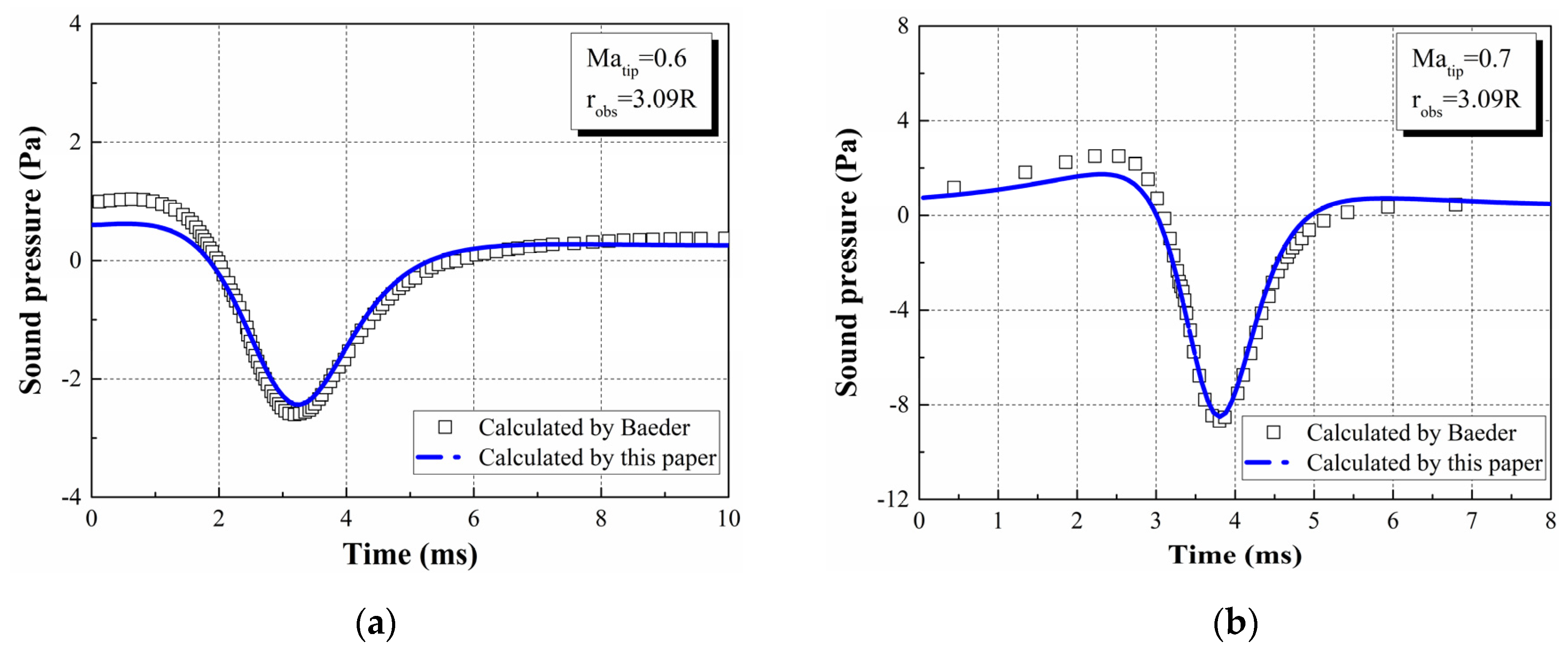
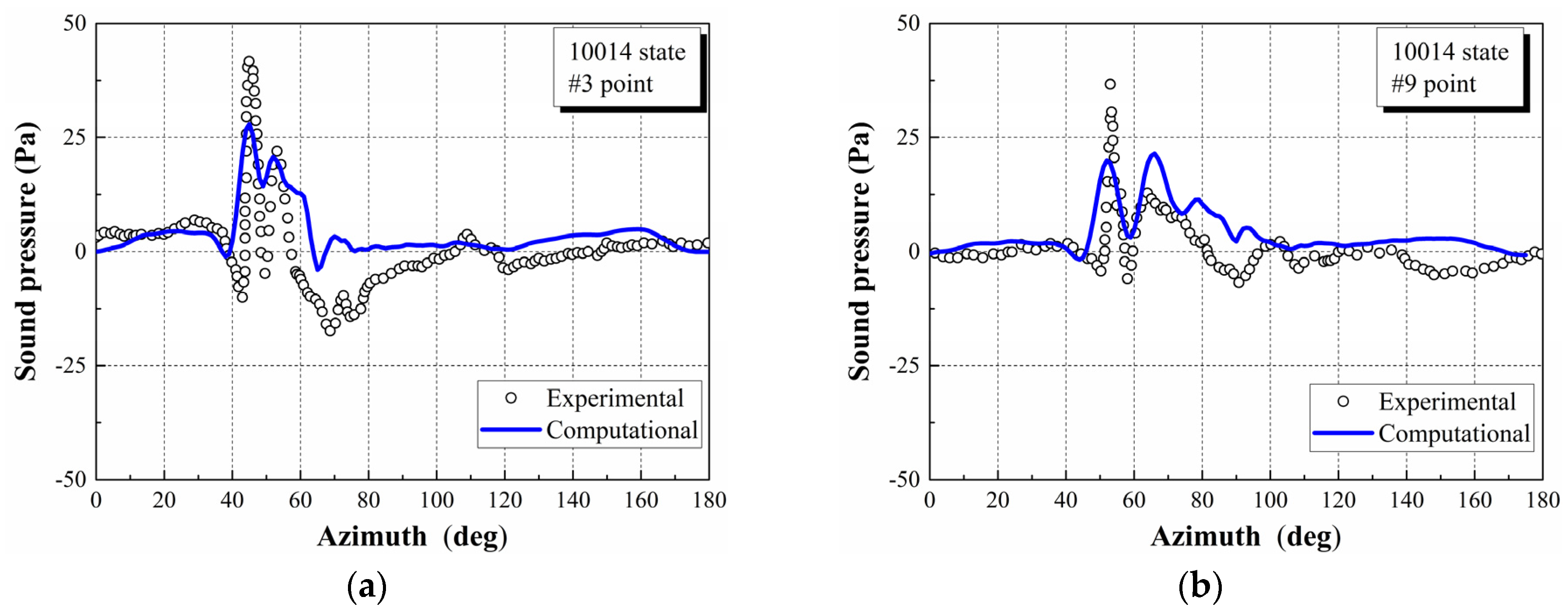
2.3. Validation Cases

The CFD solver and trim model used in this paper have been validated through different experimental cases (see Refs. [18,19]), which show reasonable accuracy in the prediction of aerodynamic performance. Current existing experiments are mostly about the aerodynamics of coaxial rotors [29,30]. There are few experimental acoustic data for coaxial rotors. For the single rotor in hover state, the noise is dominated by the thickness and loading noise components, at a low tip Mach number. The UH-1H rotor is often used for acoustic validation. Although the existing experimental data focus on high tip Mach number states, the calculated results by Baeder [31] are reliable for validation. Figure 3 shows the comparison of sound pressure results. It can be seen that results of this paper demonstrate good agreement with those of Baeder.

Figure 4 shows the experimental sound pressure of the AH-1/OLS [32] single rotor, compared with the calculated results of this paper. The state is Ma_tip = 0.664, μ = 0.164, which has obvious blade vortex interaction (BVI). At this time, the rotor works in a complex interaction flow field, and it is difficult to accurately predict the load fluctuations on the blade surface. Thus, the calculated sound pressure results have some expected errors, which is similar to the simulation of Strawn [33]. However, the main sound pressure fluctuations can be captured well.

3. Results and Discussion

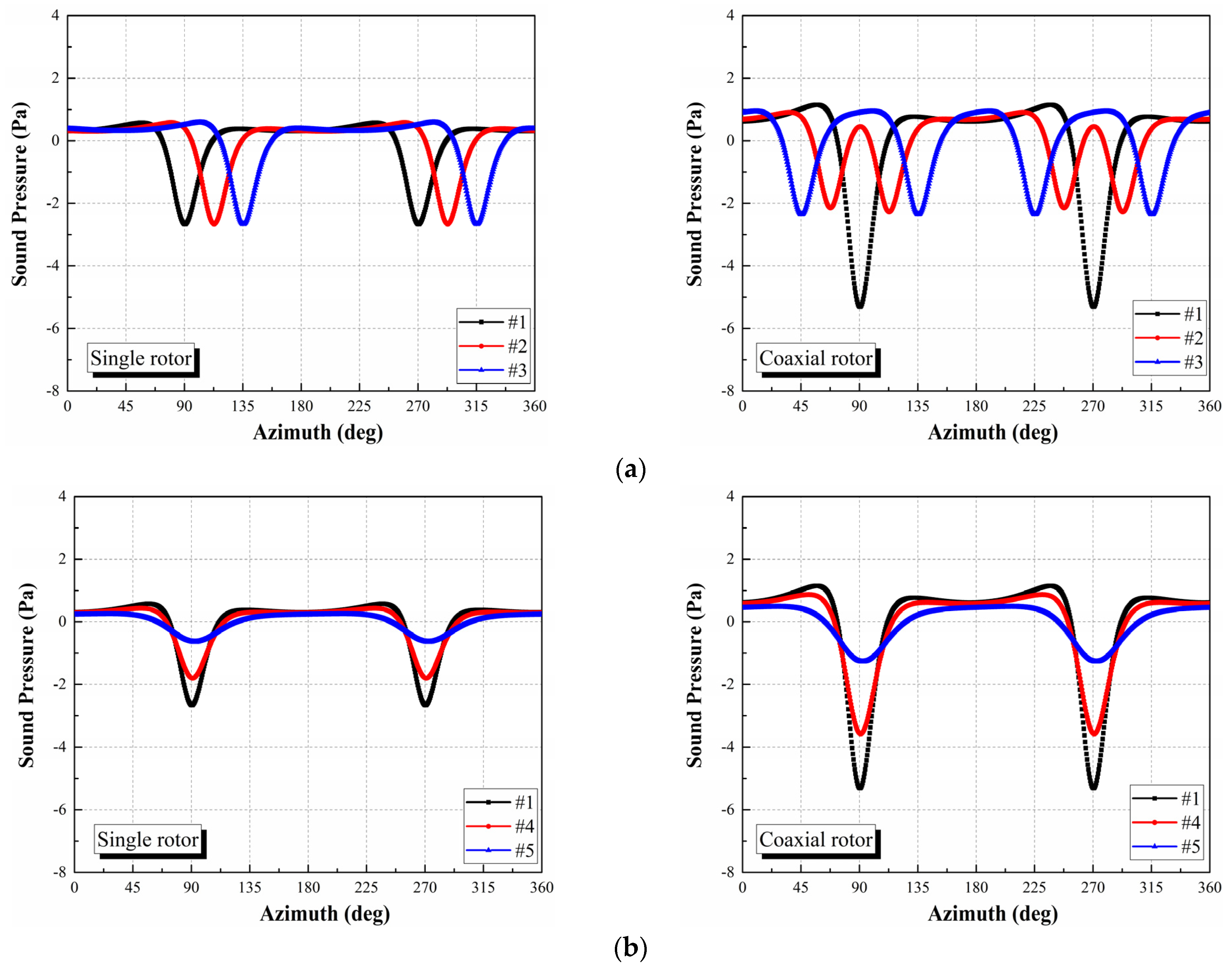
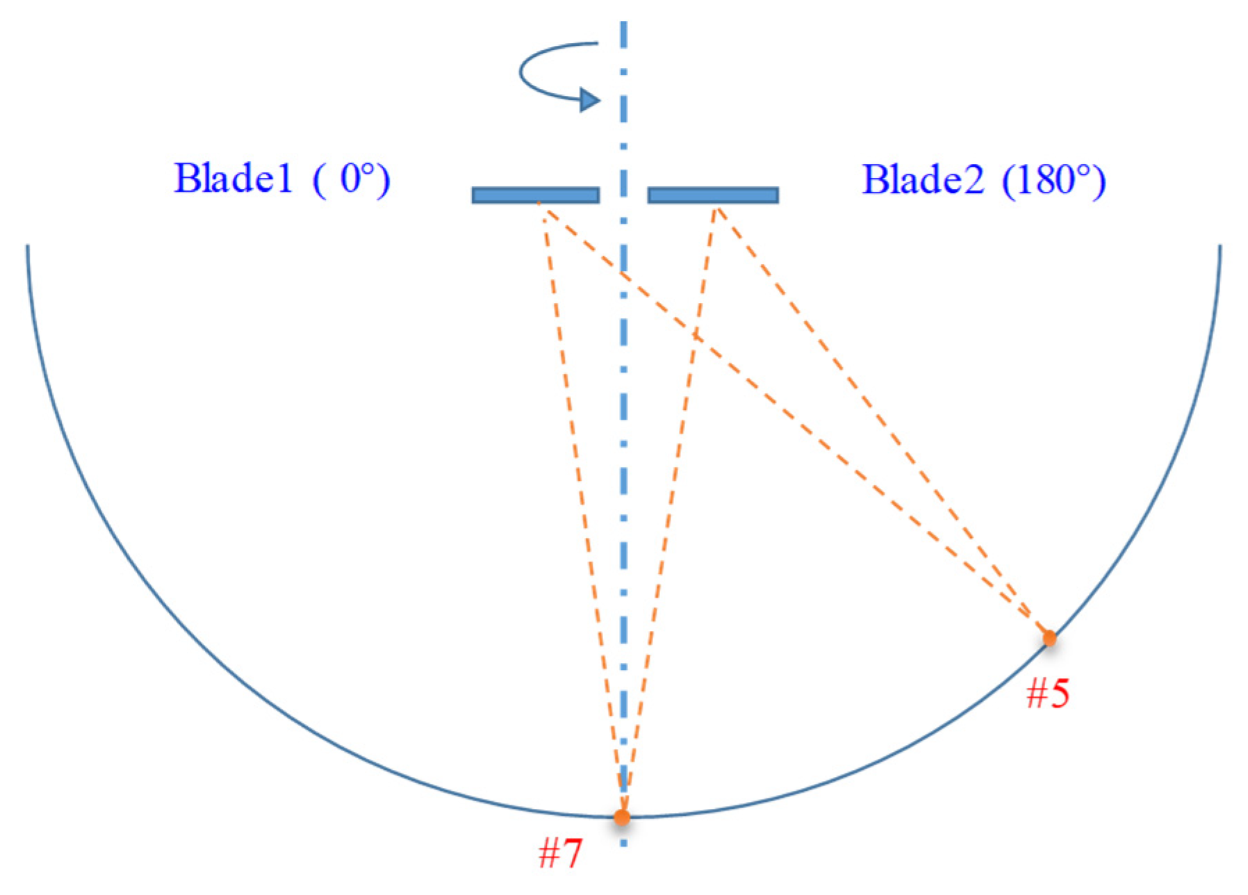
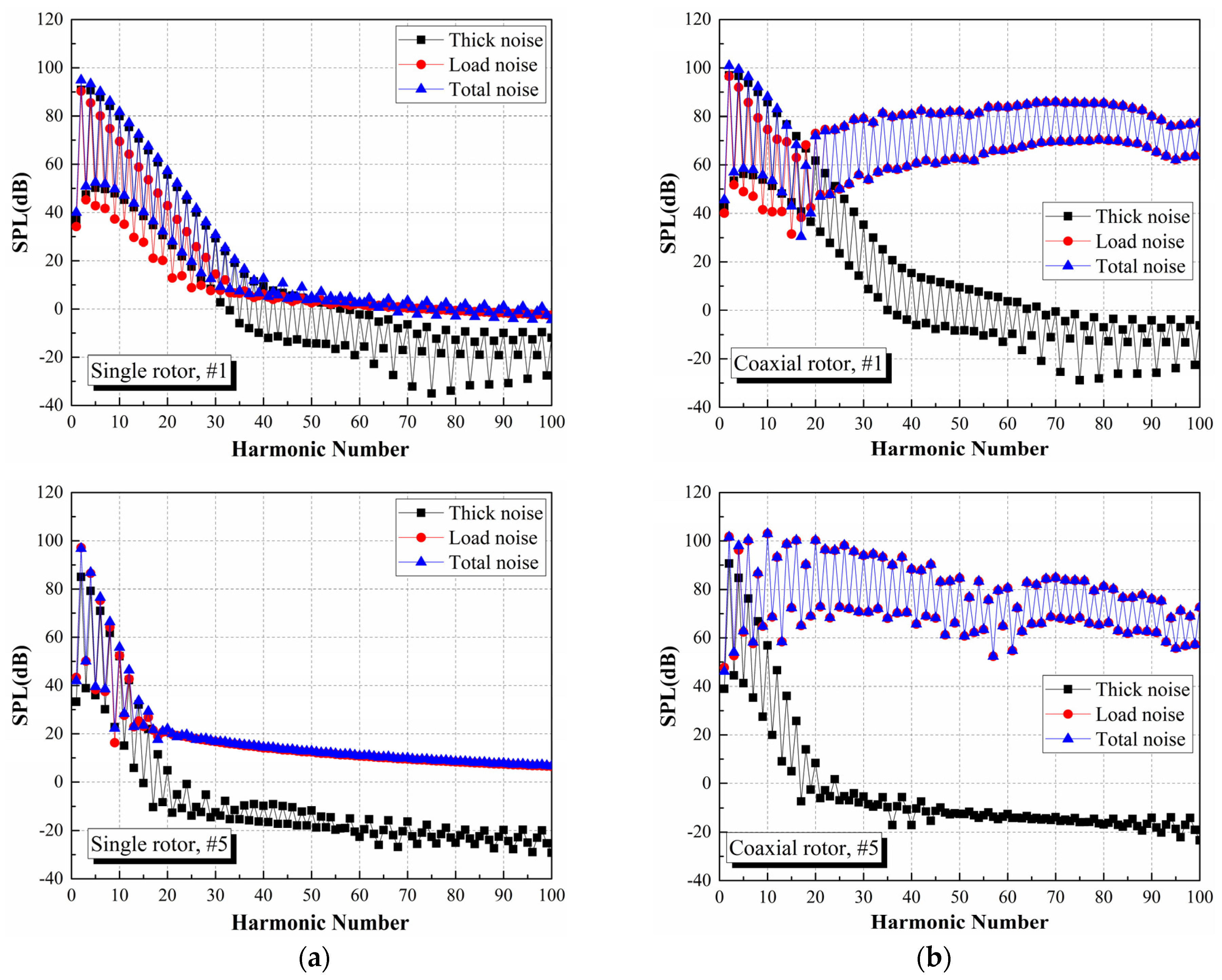
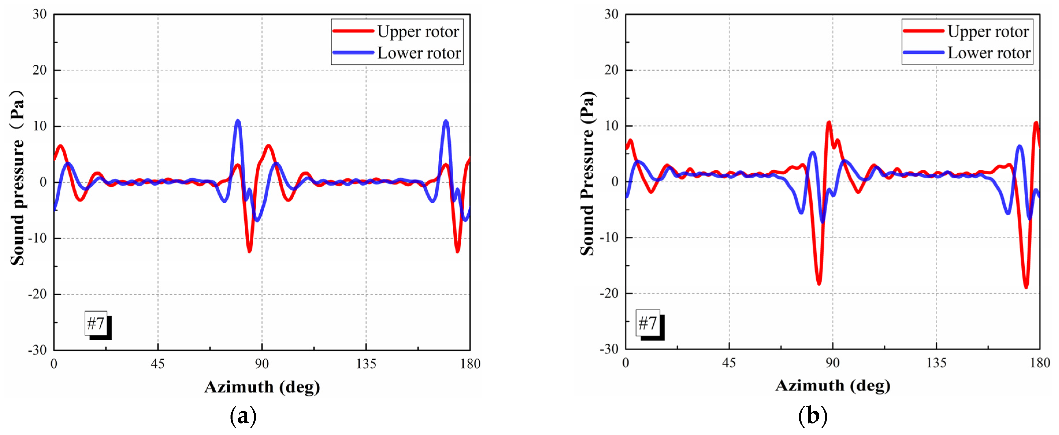
3.1. Noise at Different Observation Points

Figure 5 presents the sound pressure time histories of thickness noise for the coaxial and single rotors at different observation points of case A3. Here, the single rotor means the isolated upper rotor without the lower one, which adopts the same collective pitch as the upper rotor. It can be seen from the three observation points in the rotor plane (#1, #2, and #3) that, for the single rotor, different azimuth angles only affect the phases of the sound pressure, but have no effect on the amplitudes and waveforms. There are two troughs in one resolution, as each rotor has two blades.

For a coaxial rotor, the sound pressure history is the superposition of those caused by the twin rotors. As the rotation directions of them are opposite, the sound pressure fluctuations of the two rotors are opposite along the azimuth angle. At #1 point, the troughs are superimposed, which forms larger troughs. At #2 and #3 points, there are four troughs, but the amplitudes are slightly smaller than the single rotor, due to the superposition. Through the three observation points in the longitudinal plane (#1, #4, and #5), it can be found that, as the location moves downward from the rotor plane, the fluctuation amplitudes caused by thickness noise gradually decrease, while the waveform and phase have no change. For the coaxial rotor, the amplitudes of troughs are roughly twice those of the single rotor, due to the superposition effect of rotor noise sources.

Figure 6 shows the temporal C_T and its first-order time derivative of the coaxial and single rotors for case A3. For the single rotor, the thrust is almost constant at different azimuths, while for the dual rotors, the thrusts show periodic unsteady fluctuations. A detailed explanation of the thrust fluctuations has been given in Ref. [18]. It is important to note that there are pulse-type fluctuations at the locations where the blades meet, which can be called the blade-meeting interaction. Thrust of the upper rotor spikes down, but for the lower one, it spikes up. Moreover, the pulse amplitude of the upper rotor is much larger than the lower rotor. Referring to Equation (4), considering that rotor azimuth has no influence on $M_i$, it means that ${\dot{M}}_i$ is equal to 0. Thus, the first-order time derivative of load ($\dot{p}$) is dominant in the noise source term. As seen in Figure 6b, for the time derivative of C_T, the unsteady fluctuations mainly occur at the blade-meeting azimuths, and the fluctuation amplitudes of the upper rotor are obviously higher than those of the lower rotor.

Figure 7 shows the sound pressure histories of loading noise at different observation points for case A3. For the single rotor, blade loads are almost same at different azimuths. Thus, at #7 point, there is little load fluctuation, which corresponds to little sound pressure. According to Equation (4), the terms of $\dot{p}$ and ${\dot{M}}_i$ both are theoretically equal to 0. At other points, the sound pressures have periodic fluctuations, which is due to the changes in rotor position relative to the observation point and the radiation direction of the loading noise.

For the coaxial rotor, fluctuations in sound pressure are more complex. At #7 point,${\dot{M}}_i$ remains 0, and the sound pressure is mainly caused by the unsteady interaction loads, corresponding to a large value of $\dot{p}$. This causes a new kind of impulsive loading noise, compared with the single rotor. As rotors meet every other 90°, the main fluctuation period is also around 90°. The amplitude of impulse increases as the observation point moves down from the rotor disk plane; see #1 to #7. Moreover, for #4 and #5 points, the waveforms and phases are both different from #7 point. This will be discussed in detail below.

Figure 8 shows the comparison of loading noise sound pressures in a half rotor revolution. By comparing Figure 8b and Figure 6b, it can be found that the characteristics of sound pressure are very close to the time derivative of C_T. The main period of fluctuation is around 90°, and the amplitude of the upper rotor is larger than that of the lower rotor. As seen in Figure 8a, the wave marked as No. 2 is much weaker than No. 1, and the interval between the two troughs of the upper rotor is less than 90°. A possible explanation for the sub-sound pressure fluctuations (No. 2) is the result of the interaction between the upper rotor tip vortex and the blade of the lower rotor. This is unreasonable, considering that the vortex interaction of a coaxial rotor in hover is a kind of vertical interaction, which has little effect on the blade load.

In order to illustrate the phenomenon of the No. 2 wave, the sound pressure of loading noise at different points in the longitudinal plane is given in Figure 9. As the observation point gradually deviates from the position directly below the rotor (#7 point), the amplitude of the No. 2 wave gradually weakens, and the phase also changes. According to the position diagram of a rotor and two observation points (Figure 10), the #7 point is located directly below the rotor, and different azimuth angles have no effect on its vector distance from the rotor, which contain r and θ in Equation (4). The #5 point is located diagonally below the rotor. When the rotor is at the longitudinal azimuth, for the #5 point, the distances from blades at 0° and 180° are different from the #7 point. By comparison, for blades at 90° and 270°, their distances from #5 and #7 points are almost same. It can be concluded that the No. 1 wave is caused by the load fluctuations of blades at 90° and 270°; for different observation points, the phases are almost the same, while the amplitude and waveform have some change due to the radiation direction of the loading noise. The No. 2 wave is caused by load fluctuations at 0° and 180°, leading to the differences in the waveform and phase among different observation points.

Figure 11 shows the sound pressure level (SPL) frequency spectrum of loading noise at different observation points. The fundamental frequency corresponds to the rotor rotation speed, i.e., f₀ = 15.915 Hz. As the rotors are two-bladed, the blade-pass frequency (BPF) is twice f₀. At the #1 point, the thickness noise of the coaxial rotor is similar to the single rotor. The strong magnitude frequencies are mainly integer multiples of BPF. For the single rotor, the total noise is dominated by the thickness noise, and the amplitude of loading noise in the high-frequency band decreases rapidly. For the coaxial rotor, the total noise is dominated by the thickness noise before the 20th harmonic, while, above this, the total noise is dominated by the loading noise. At the #5 point, the thickness noise is much weaker than the loading noise, as it mainly transmits in the rotor disk plane. Compared with the single rotor, the loading noise of the coaxial rotor has a stronger magnitude in a larger range of the frequency band. The total noise is mainly dominated by the loading noise, both in low-frequency and high-frequency bands. It is well known that the loading noise frequency of a single rotor is usually low [34], and in the high-frequency band, the magnitude is rather weak. As seen in the figures, on one hand, the aerodynamic interaction of the coaxial rotor leads to stronger loading noise. On the other hand, the features of the frequency spectrum have been changed. The noise in the high-frequency band is enhanced, which is obviously different from the single rotor.

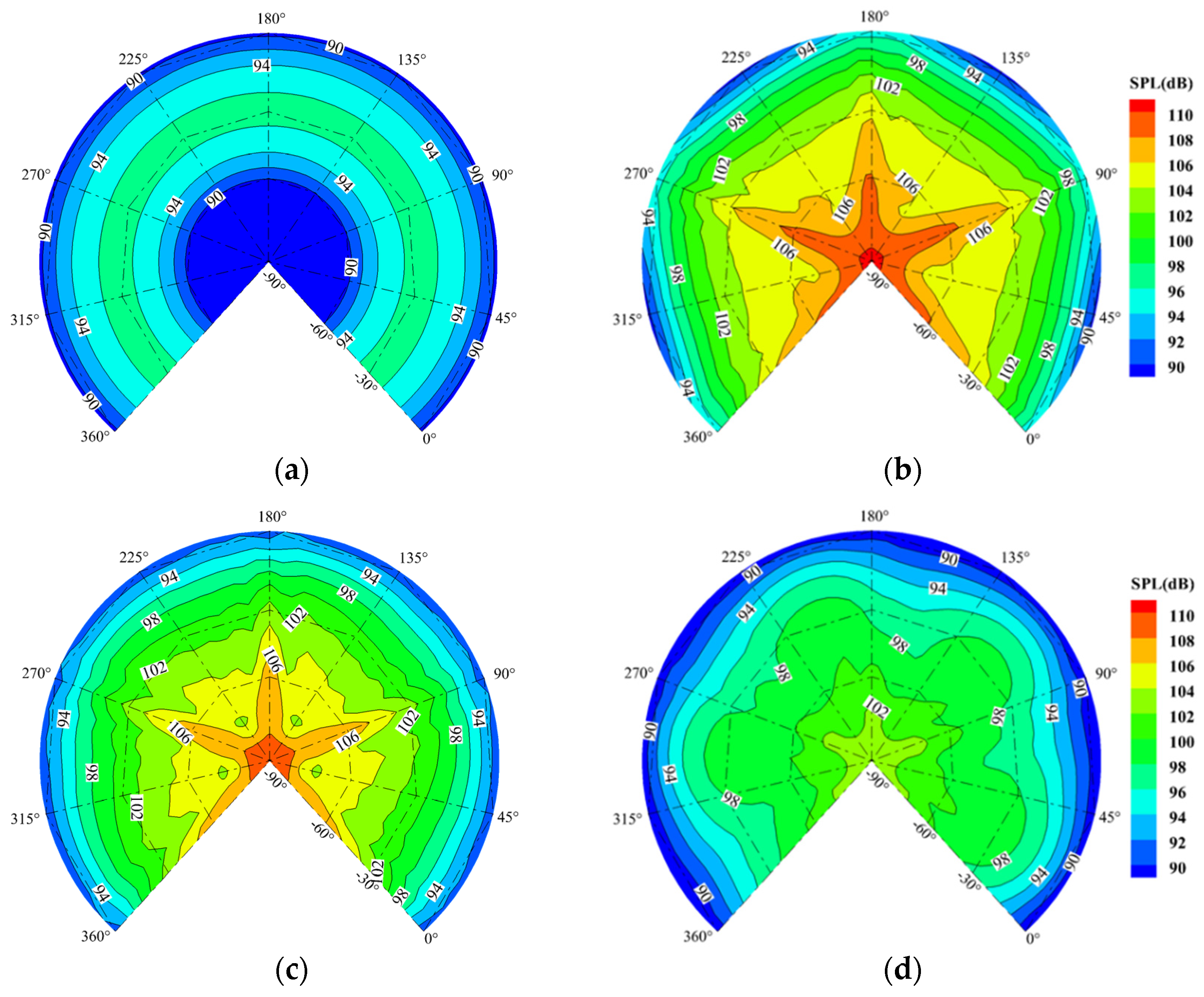
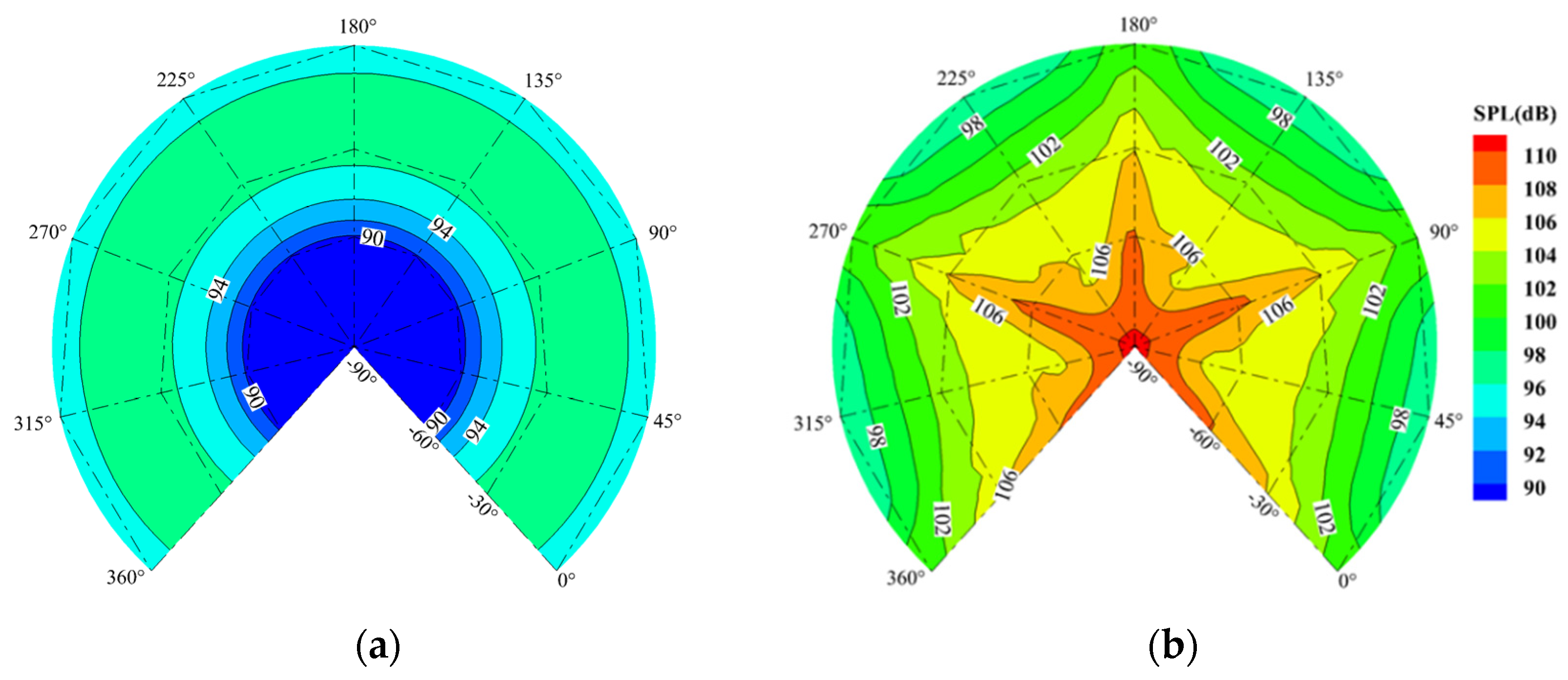
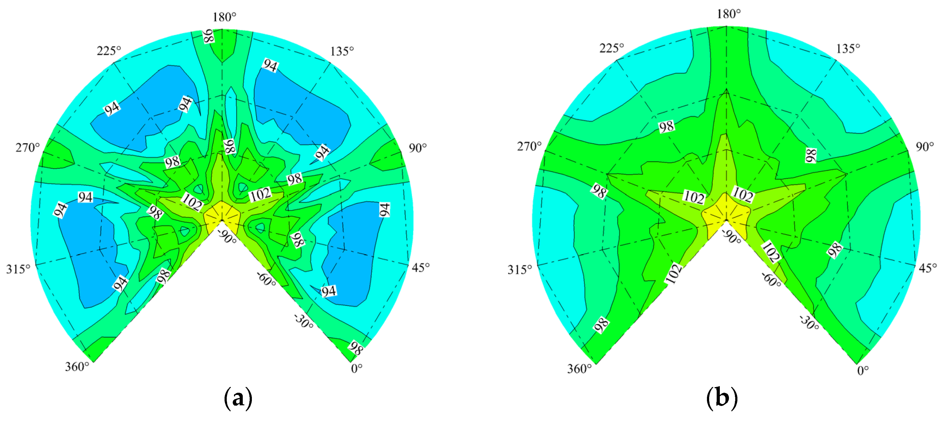
3.2. Noise Radiation Characteristics

Figure 12 shows the thickness noise SPL contour map. It can be seen that the thickness noise of a single rotor is distributed in concentric circles on the hemisphere surface. The noise of the coaxial rotor shows a periodic distribution with the azimuth angle. Moreover, around the blade-meeting azimuths, the noise is enhanced, due to the source superposition of the two rotors. The minimum SPL is located immediately below the rotor hub center, which is similar to the single rotor.

The comparison of loading noise SPL distributions between the coaxial rotor and the single rotor is shown in Figure 13. The SPL of loading noise increases significantly near the azimuths where the twin rotors meet each other. This is consistent with the fluctuation characteristics of the rotor load in hover. The intensity of loading noise caused by the upper rotor is obviously stronger than the lower rotor. It should be noted that the strongest loading noise of the single rotor occurs at an approximately −30° latitude angle. For the coaxial rotor, the noise intensity increases with the approach to the bottom of the sound radiation hemisphere, which reaches the maximum at the bottom of the sphere (−90° latitude angle). It should be noted that, for the single rotor, the noise of the point immediately below the rotor center is the lowest one, while for the coaxial rotor, it is the highest location. This is mainly determined by the unsteady interaction loads of the coaxial rotor.

The total noise SPL results of the coaxial and single rotors are given in Figure 14. Combined with the distribution of loading noise in Figure 13, it can be seen that the contribution of thickness noise mainly distributes near the rotor disk plane. In addition, the loading noise is dominant on the sound radiation hemisphere deviating from the rotor disk plane. Moreover, the dominant effect of the coaxial rotor loading noise on the total noise is more obvious. This is consistent with the previous analysis of the noise radiation characteristics of the observation points at different locations.

3.3. Comparison of Different C_T Levels

The research is conducted at three different C_T levels, as listed in Table 2. Figure 15 shows the comparison of loading sound pressure at different C_T levels. For the A0 case, as the airfoil of blades is symmetrical and the collective pitches of the twin rotors are both zero, the rotor thrusts almost remain constant most of the time, while they show impulsive fluctuations at blade-meeting azimuths. The thrust of the upper rotor spikes down, while the lower rotor thrust spikes up, as illustrated in Ref. [18]. Correspondingly, the sound pressure fluctuations of the upper and lower rotors are almost antisymmetric in the A0 case. As C_T increases, the impulsive fluctuation of the upper rotor becomes stronger, while for the lower rotor, the change is not obvious. This is consistent with the changes in impulsive thrust fluctuation with different C_T levels, as discussed in Ref. [18]. Combined with the above results, it can be concluded that the impulsive noise of the coaxial rotor is mainly caused by the blade-meeting interaction, rather than the interaction between the upper rotor vortex and the lower rotor blade.

Figure 16 shows the total noise distribution of the coaxial rotor at different C_T levels. It is easy to find that the total noise SPL becomes stronger with the increase in C_T. This is because the load fluctuations caused by the aerodynamic interaction are stronger. For the A0 case, there is a low-SPL region near the latitude angle of −30°, between every two blade-meeting azimuths, marked in blue in the figure. This is because the thickness noise mainly radiates in the rotor disk plane, and the loading noise is only strong at blade-meeting azimuths for the A0 case. Thus, the superposition of the thickness and loading noises leads to the four low-SPL regions. For the A1 case, the loading noise caused by the interaction is stronger and spreads from the blade-meeting azimuths to the surrounding region. The result is that the low-SPL region lies near the rotor disk plane, between every two blade-meeting azimuths.

4. Conclusions

A CFD solver based on RANS equations and a high-efficiency trim method is established to simulate the unsteady loads of a two-bladed coaxial rotor in hover. Farassat 1A formulations are applied to predict the thickness and loading noise. The acoustic characteristics of the coaxial rotor are analyzed compared with the single rotor. The following conclusions can be drawn:

(1) The noise of the coaxial rotor is rather different from a single rotor in the characteristics of the radiation and spectrum. This is mainly caused by two factors. One is the noise superposition effect of the upper and lower rotors, which are contra-rotating. The other is the complex unsteady aerodynamic interaction, especially the unsteady impulsive loads induced by the blade-meeting interaction, which leads to a new kind of impulsive loading noise.

(2) The thickness noise of a single rotor distributes as concentric rings, which remains constant at different azimuths. Due to the noise superposition effect, the thickness noise SPL of a coaxial rotor shows cyclical fluctuations along the latitude (azimuth) angle. Moreover, at the blade-meeting azimuth angles, the magnitudes of thickness noise are enhanced.

(3) For the single rotor, the highest SPL region of loading noise lies obliquely below the rotor disk, at an approximately -30° latitude angle. For the coaxial rotor, the highest SPL region is immediately below the rotor disk center. This is due to the fact that the noise of the coaxial rotor is mainly determined by the unsteady interaction loads, which causes the strongest noise below the rotor. The loading noise around the blade-meeting azimuths is also enhanced.

(4) Regarding the frequency spectrum, for the single rotor, the frequency of loading noise is mainly lower than the 40th harmonic of rotor rotation frequency, in this paper. For the coaxial rotor, the loading noise shows much stronger magnitude than the single rotor in the high-frequency band, due to the high-frequency unsteady interaction loads.

References

1. Ho, J.C.; Yeo, H. Analytical study of an isolated coaxial rotor system with lift offset. Aerosp. Sci. Technol. 2020, 100, 105818. [Google Scholar] [CrossRef]
2. Burgess, R.K. The ABC™ Rotor—A historical perspective. In Proceedings of the 60th American Helicopter Society Annual Forum, Baltimore, MD, USA, 7–10 June 2004. [Google Scholar]
3. Bagai, A. Aerodynamic design of the X2 technology demonstrator main rotor blade. In Proceedings of the 64th American Helicopter Society Annual Forum, Montréal, QC, Canada, 29 April—1 May 2008; pp. 29–44. [Google Scholar]
4. Lakshminarayan, V.K.; Baeder, J.D. Computational investigation of microscale coaxial-rotor aerodynamics in hover. J. Aircr. 2010, 47, 940–955. [Google Scholar] [CrossRef] [Green Version]
5. Hayami, K.; Sugawara, H.; Tanabe, Y.; Kameda, M. Numerical investigation of aerodynamic interference on coaxial rotor. In Proceedings of the AIAA Scitech 2020 Forum, Orlando, FL, USA, 6–10 January 2020. [Google Scholar]
6. Shirey, J.; Brentner, K.; Chen, H.-n. A validation study of the PSU-WOPWOP rotor noise prediction code. In Proceedings of the 45th AIAA Aerospace Sciences Meeting and Exhibit, Reno, NV, USA, 8–11 January 2007. [Google Scholar]
7. Wachspress, D.A.; Quackenbush, T.R. Impact of rotor design on coaxial rotor performance, wake geometry and noise. In Proceedings of the 62th American Helicopter Society Annual Forum, Phoenix, AZ, USA, 9–11 May 2006; pp. 41–63. [Google Scholar]
8. Kim, H.W.; Duraisamy, K.; Brown, R.E. Effect of rotor stiffness and lift offset on the aeroacoustics of a coaxial rotor in level flight. In Proceedings of the 65th American Helicopter Society Annual Forum, Grapevine, TX, USA, 27–29 May 2009; pp. 1–21. [Google Scholar]
9. Kim, H.W.; Kenyon, A.R.; Duraisamy, K.; Brown, R.E. Interactional aerodynamics and acoustics of a hingeless coaxial helicopter with an auxiliary propeller in forward flight. Aeronaut. J. 2009, 113, 65–78. [Google Scholar] [CrossRef] [Green Version]
10. Klimchenko, V.; Sridharan, A.; Baeder, J.D. CFD/CSD study of the aerodynamic interactions of a coaxial rotor in high-speed forward flight. In Proceedings of the 35th AIAA Applied Aerodynamics Conference, Denver, CO, USA, 5–9 June 2017; pp. 1–22. [Google Scholar]
11. Passe, B.J.; Sridharan, A.; Baeder, J.D. Computational investigation of coaxial rotor interactional aerodynamics in steady forward flight. In Proceedings of the 33rd AIAA Applied Aerodynamics Conference, Dallas, TX, USA, 22–26 June 2015; pp. 1–29. [Google Scholar]
12. Walsh, G.; Brentner, K.; Jacobellis, G.; Gandhi, F. An acoustic investigation of a coaxial helicopter in high-speed flight. In Proceedings of the 72nd American Helicopter Society Annual Forum, Fairfax, VA, USA, 17 May 2016. [Google Scholar]
13. Zhu, Z.; Zhao, Q.; Chen, S.; Wang, B. Analyses on aeroacoustic characteristics of coaxial rotors in hover. Acta Acust. 2016, 41, 833–842. [Google Scholar] [CrossRef]
14. Wang, B.; Cao, C.; Zhao, Q.; Yuan, X.; Zhu, Z. Aeroacoustic Characteristic Analyses of Coaxial Rotors in Hover and Forward Flight. Int. J. Aeronaut. Space Sci. 2021, 22, 1278–1292. [Google Scholar] [CrossRef]
15. Jia, Z.; Lee, S.; Sharma, K.; Brentner, K.S. Aeroacoustic analysis of a lift-offset coaxial rotor using high-fidelity CFD-CSD loose coupling simulation. In Proceedings of the 74th American Helicopter Society Annual Forum, Phoenix, AZ, USA, 14–17 May 2018; pp. 1–21. [Google Scholar]
16. Jia, Z.; Lee, S. Impulsive Loading Noise of a Lift-Offset Coaxial Rotor in High-Speed Forward Flight. AIAA J. 2020, 58, 687–701. [Google Scholar] [CrossRef]
17. Jia, Z.; Lee, S. Aerodynamically induced noise of a lift-offset coaxial rotor with pitch attitude in high-speed forward flight. J. Sound Vib. 2021, 491, 115737. [Google Scholar] [CrossRef]
18. Qi, H.; Xu, G.; Lu, C.; Shi, Y. A study of coaxial rotor aerodynamic interaction mechanism in hover with high-efficient trim model. Aerosp. Sci. Technol. 2019, 84, 1116–1130. [Google Scholar] [CrossRef]
19. Qi, H.; Xu, G.; Lu, C.; Shi, Y. Computational investigation on unsteady loads of high-speed rigid coaxial rotor with high-efficient trim model. Int. J. Aeronaut. Space Sci. 2019, 20, 16–30. [Google Scholar] [CrossRef]
20. Farassat, F. Linear acoustic formulas for calculation of rotating blade noise. AIAA J. 1981, 19, 1122–1130. [Google Scholar] [CrossRef]
21. Pomin, H.; Wagner, S. Navier-Stokes analysis of helicopter rotor aerodynamics in hover and forward flight. J. Aircr. 2002, 39, 813–821. [Google Scholar] [CrossRef]
22. Van Leer, B. Towards the ultimate conservative difference scheme. V. A second-order sequel to Godunov’s method. J. Comput. Phys. 1979, 32, 101–136. [Google Scholar] [CrossRef]
23. Spalart, P.; Allmaras, S. A one-equation turbulence model for aerodynamic flows. In Proceedings of the 30th Aerospace Sciences Meeting and Exhibit, Reno, NV, USA, 6–9 January 1992; pp. 1–22. [Google Scholar]
24. Yoon, S.; Jameson, A. Lower-upper Symmetric-Gauss-Seidel method for the Euler and Navier-Stokes equations. AIAA J. 1988, 26, 1025–1026. [Google Scholar] [CrossRef] [Green Version]
25. Ye, Z.; Xu, G.; Shi, Y.; Xia, R. A high-efficiency trim method for CFD numerical calculation of helicopter rotors. Int. J. Aeronaut. Space Sci. 2017, 18, 186–196. [Google Scholar] [CrossRef]
26. Lyu, W.; Wang, S.; Yang, A. Some improvements of hybrid trim method for a helicopter rotor in forward flight. Aerosp. Sci. Technol. 2021, 113, 106709. [Google Scholar] [CrossRef]
27. Zhao, Y.; Shi, Y.; Xu, G. Helicopter Blade-Vortex Interaction Airload and Noise Prediction Using Coupling CFD/VWM Method. Appl. Sci. 2017, 7, 381. [Google Scholar] [CrossRef] [Green Version]
28. Shi, Y.; Li, T.; He, X.; Dong, L.; Xu, G. Helicopter Rotor Thickness Noise Control Using Unsteady Force Excitation. Appl. Sci. 2019, 9, 1351. [Google Scholar] [CrossRef] [Green Version]
29. Feil, R.; Rauleder, J.; Cameron, C.G.; Sirohi, J. Aeromechanics analysis of a high-advance-ratio lift-offset coaxial rotor system. J. Aircr. 2019, 56, 166–178. [Google Scholar] [CrossRef]
30. Silwal, L.; Raghav, V. Preliminary study of the near wake vortex interactions of a coaxial rotor in hover. In Proceedings of the AIAA Scitech 2020 Forum, Orlando, FL, USA, 6–10 January 2020. [Google Scholar]
31. Baeder, J.D.; Gallman, J.M.; Yu, Y.H. A computational study of the aeroacoustics of rotors in hover. J. Am. Helicopter Soc. 1993, 42, 39–53. [Google Scholar] [CrossRef]
32. Yu, Y.H.; Tung, C.; Gallman, J.; Schultz, K.J.; Wall, B.v.d.; Spiegel, P.; Michea, B. Aerodynamics and acoustics of rotor blade-vortex interactions. J. Aircr. 1995, 32, 970–977. [Google Scholar] [CrossRef]
33. Strawn, R.C.; Duque, E.P.N.; Ahmad, J. Rotorcraft aeroacoustics computations with overset-grid CFD methods. J. Am. Helicopter Soc. 1999, 44, 132–140. [Google Scholar] [CrossRef]
34. Brentner, K.S.; Farassat, F. Modeling aerodynamically generated sound of helicopter rotors. Prog. Aerosp. Sci. 2003, 39, 83–120. [Google Scholar] [CrossRef] [Green Version]
Figure 1. Moving overset mesh system for the coaxial rotor.
Applsci 12 02813 g001
Figure 2. Schematic diagram of acoustic radiation hemisphere and Lambert projection of rigid coaxial rotor. (a) Acoustic radiation hemisphere; (b) Lambert projection map.
Applsci 12 02813 g002
Figure 3. Sound pressure history of UH-1H rotor at low Mach number. (a) Matip = 0.6; (b) Matip = 0.7.
Applsci 12 02813 g003
Figure 4. Comparison of calculated sound pressure and experimental data. (a) #3 point; (b) #9 point.
Applsci 12 02813 g004
Figure 5. Sound pressure histories of thickness noise. (a) Points in the rotor disk plane; (b) Points in the longitudinal plane.
Applsci 12 02813 g005
Figure 6. Comparison of temporal rotor performance. (a) CT; (b) dCT/dt.
Applsci 12 02813 g006
Figure 7. Loading noise at different observation points. (a) Single rotor; (b) Coaxial rotor.
Applsci 12 02813 g007
Figure 8. Loading noise sound pressures at #5 and #7 points. (a) #5 point; (b) #7 point.
Applsci 12 02813 g008
Figure 9. Comparison of loading noise at different observation points. (a) Upper rotor; (b) Lower rotor.
Applsci 12 02813 g009
Figure 10. Schematic diagram of distances between observation points and blades (ψ = 0°).
Applsci 12 02813 g010
Figure 11. Frequency spectrum of loading noise at different observation points. (a) Single rotor; (b) Coaxial rotor.
Applsci 12 02813 g011
Figure 12. Thickness noise SPL contour maps. (a) Single rotor; (b) Coaxial rotor.
Applsci 12 02813 g012
Figure 13. Loading noise SPL contour maps. (a) Single rotor; (b) Coaxial rotor; (c) Upper rotor; (d) Lower rotor.
Applsci 12 02813 g013
Figure 14. Total noise SPL contour maps. (a) Single rotor; (b) Coaxial rotor.
Applsci 12 02813 g014
Figure 15. Sound pressures of loading noise at different CT levels. (a) A0 case; (b) A1 case.
Applsci 12 02813 g015
Figure 16. Total noise SPL contour maps of different CT levels. (a) A0 case; (b) A1 case.
Applsci 12 02813 g016